Download as PDF, PPTX
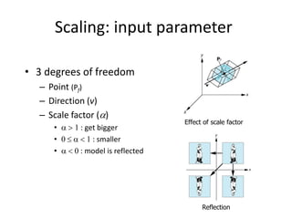
![Modeling a Cube
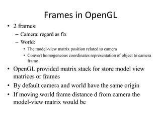
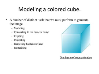
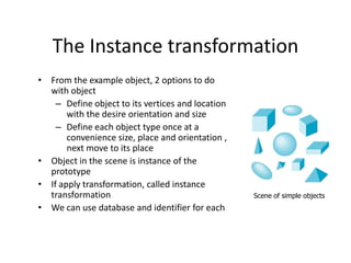
• Model as 6 planes intersection or six polygons as cube facets
• Ex. of cube definition
GLfloat vertices[8][3] = {
{-1.0,-1.0,-1.0}, {1.0,-1.0,-1.0},
{1.0,1.0,-1.0}, {-1.0,1.0,-1.0},
{-1.0,-1.0,1.0}, {1.0,-1.0,1.0},
{1.0,1.0,1.0}, {-1.0,1.0,1.0}
};
// or
typedef point3[3];
// then may define as
point3 vertices[8] = {
{-1.0,-1.0,-1.0}, {1.0,-1.0,-1.0},
{1.0,1.0,-1.0}, {-1.0,1.0,-1.0},
{-1.0,-1.0,1.0}, {1.0,-1.0,1.0},
{1.0,1.0,1.0}, {-1.0,1.0,1.0}
};
// object may defined as
void polygon(int a, int b, int c , int d) {
/* draw a polygon via list of vertices */
glBegin(GL_POLYGON);
glVertex3fv(vertices[a]);
glVertex3fv(vertices[b]);
glVertex3fv(vertices[c]);
glVertex3fv(vertices[d]);
glEnd();
}](https://image.slidesharecdn.com/geometricobjectsandtransformations-140306095054-phpapp01/85/Geometric-objects-and-transformations-7-320.jpg)
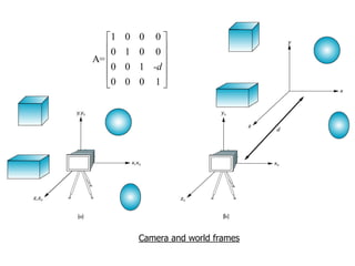
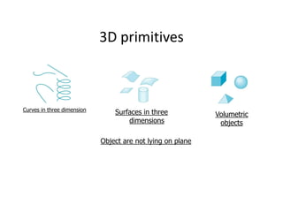
![The color cube
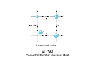
• Color to vertex list -> color 6 faces
• Define function “quad” for drawing quadrilateral polygon
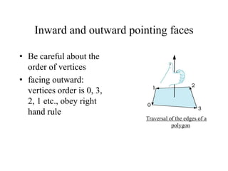
• Next define 6 faces, be careful about define outwarding
Glfloat vertices[8][3] = {{-1.0,-1.0, 1.0},{-1.0, 1.0, 1.0}, {1.0,1.0, 1.0}, {1.0,-1.0, 1.0},
{-1.0,-1.0,-1.0}, {1.0,-1.0,-1.0}, {1.0,1.0,-1.0}, {-1.0,1.0,-1.0}};
GLfloat colors[8][3] = {{0.0,0.0,0.0},{1.0,0.0,0.0}, {1.0,1.0,0.0}, {0.0,1.0,0.0},
{0.0,0.0,1.0}, {1.0,0.0,1.0}, {1.0,1.0,1.0}, {0.0,1.0,1.0}};
void quad(int a, int b, int c , int d) {
glBegin(GL_QUADS);
glColor3fv(colors[a]); glVertex3fv(vertices[a]); glColor3fv(colors[b]); glVertex3fv(vertices[b]);
glColor3fv(colors[c]); glVertex3fv(vertices[c]); glColor3fv(colors[d]); glVertex3fv(vertices[d]);
glEnd();
}
void colorcube() {
quad(0, 3, 2, 1); quad(2, 3, 7, 6); quad(0, 4, 7, 3); quad(1, 2, 6, 5); quad(4, 5, 6, 7); quad(0, 1, 5, 4);
}](https://image.slidesharecdn.com/geometricobjectsandtransformations-140306095054-phpapp01/85/Geometric-objects-and-transformations-11-320.jpg)
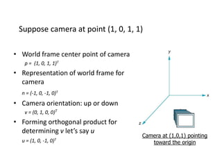
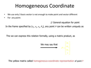
![// The arrays are the same as before and can be set up as globals:
GLfloat vertices[] = {{-1,-1,-1}, {1,-1,1}, {1,1,-1}, {-1,1,-1},{-1,-1,1}, {1,-1,1}, {1,1,1}, {-1,1,1}};
GLfloat colors[] = {{0,0,0}, {1,0,0},{1,1,0},{0,1,0},{0,0,1},{1,0,1}, {1,1,1},{0,1,1}};
// Next identify where the arrays are by
glVertexPointer(3, GL_FLOAT, 0, vertices);
glColorPointer(3, GL_FLOAT, 0, colors);
// Define the array to hold the 24 order of vertex indices for 6 faces
GLubyte cubeIndices[24] = {0,3,2,1, 2,3,7,6, 0,4,7,3, 1,2,6,5,
4,5,6,7,
0,1,5,4};
glDrawElements(type, n, format, pointer);
for (i=0; i<6; i++)
glDrawElement(GL_POLYGON, 4, GL_UNSIGNED_BYTE, &cubeIndex[4*i]};
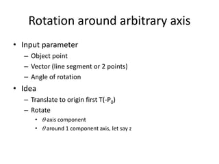
// Do better by seeing each face as quadrilateral polygon
glDrawElements(GL_QUADS, 24, GL_UNSIGNED_BYTE, cubeIndices);
// GL_QUADS starts a new quadrilateral after each four vertices](https://image.slidesharecdn.com/geometricobjectsandtransformations-140306095054-phpapp01/85/Geometric-objects-and-transformations-13-320.jpg)
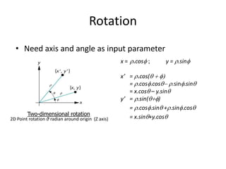
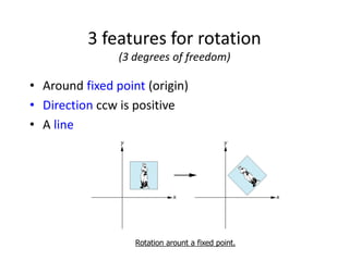
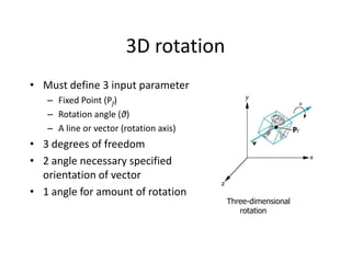
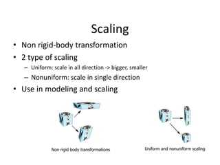
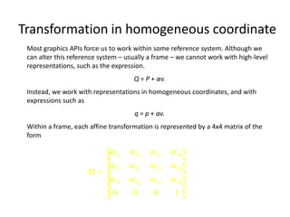
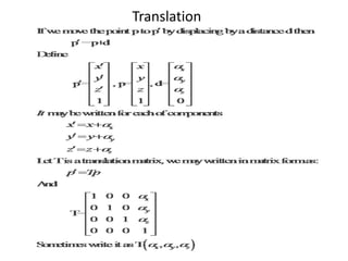
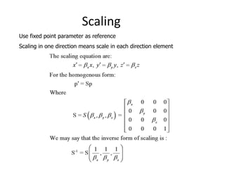
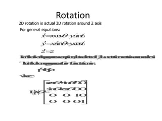
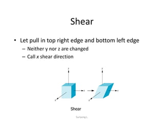
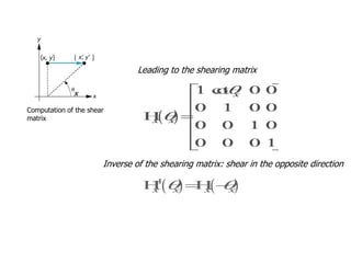
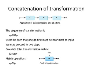
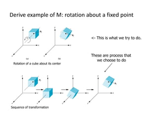
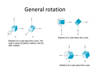
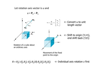
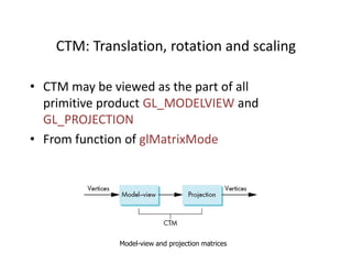
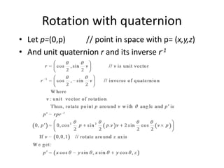
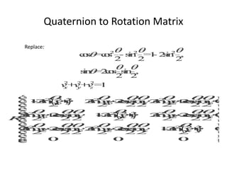

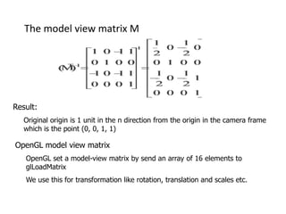
OpenGL uses model-view and projection matrices to apply transformations like translation, rotation, and scaling. The document discusses constructing transformation matrices for different types of transformations, including translation, rotation around fixed points and arbitrary axes, scaling, and shearing. It also covers combining multiple transformations using matrix multiplication and storing transformations in the current transformation matrix.