Download as PDF, PPTX

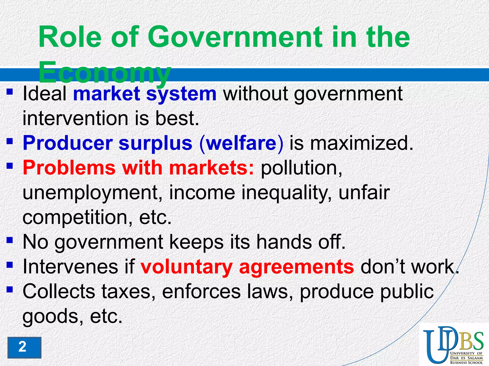
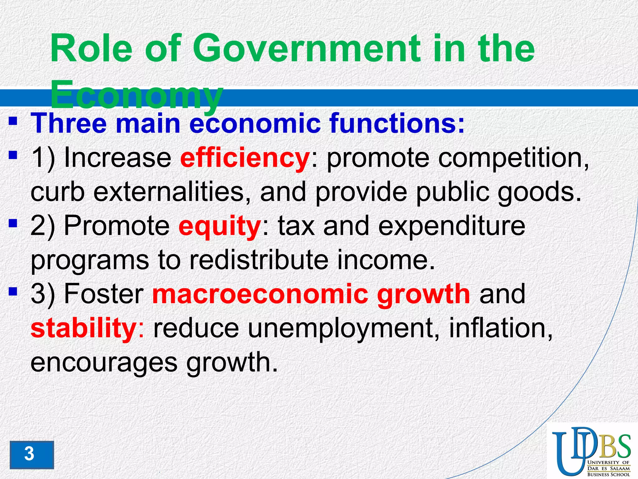

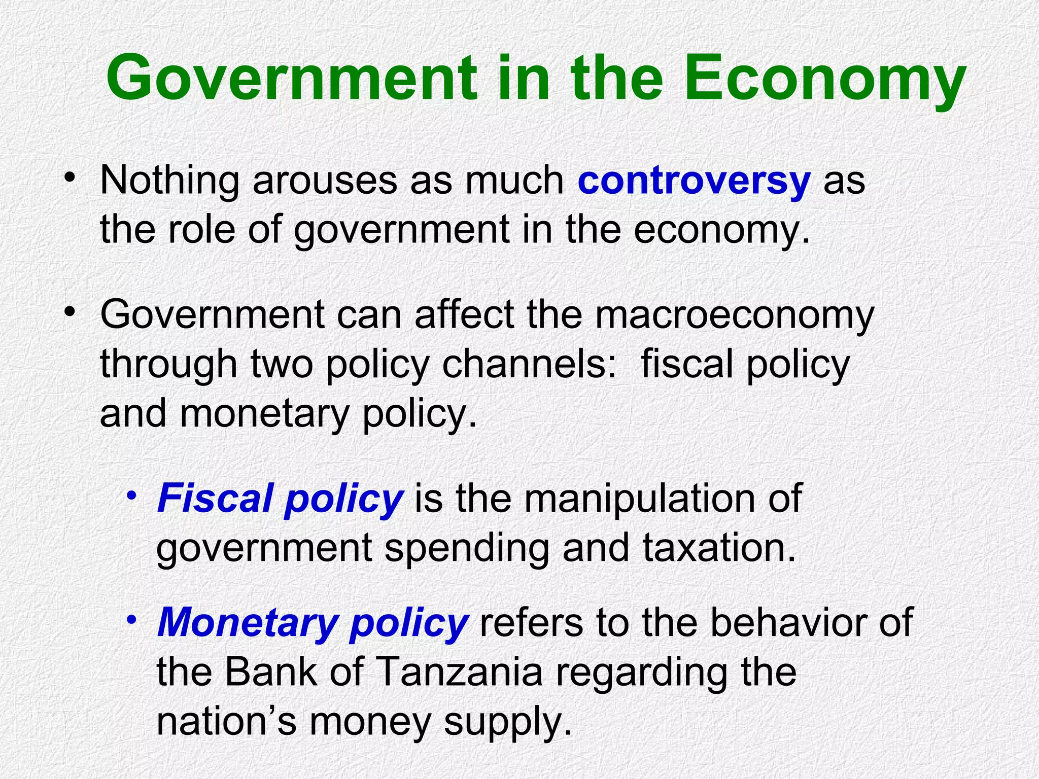
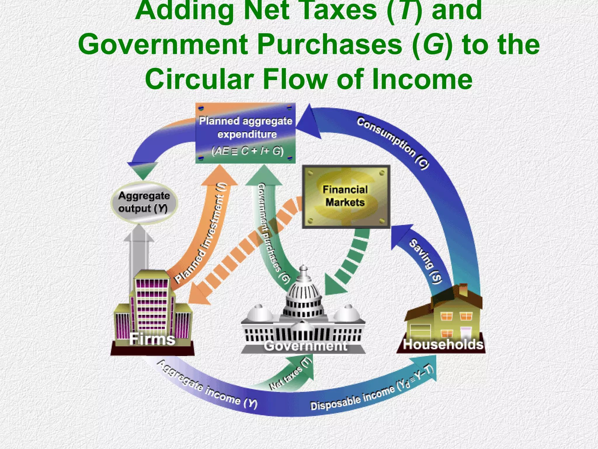


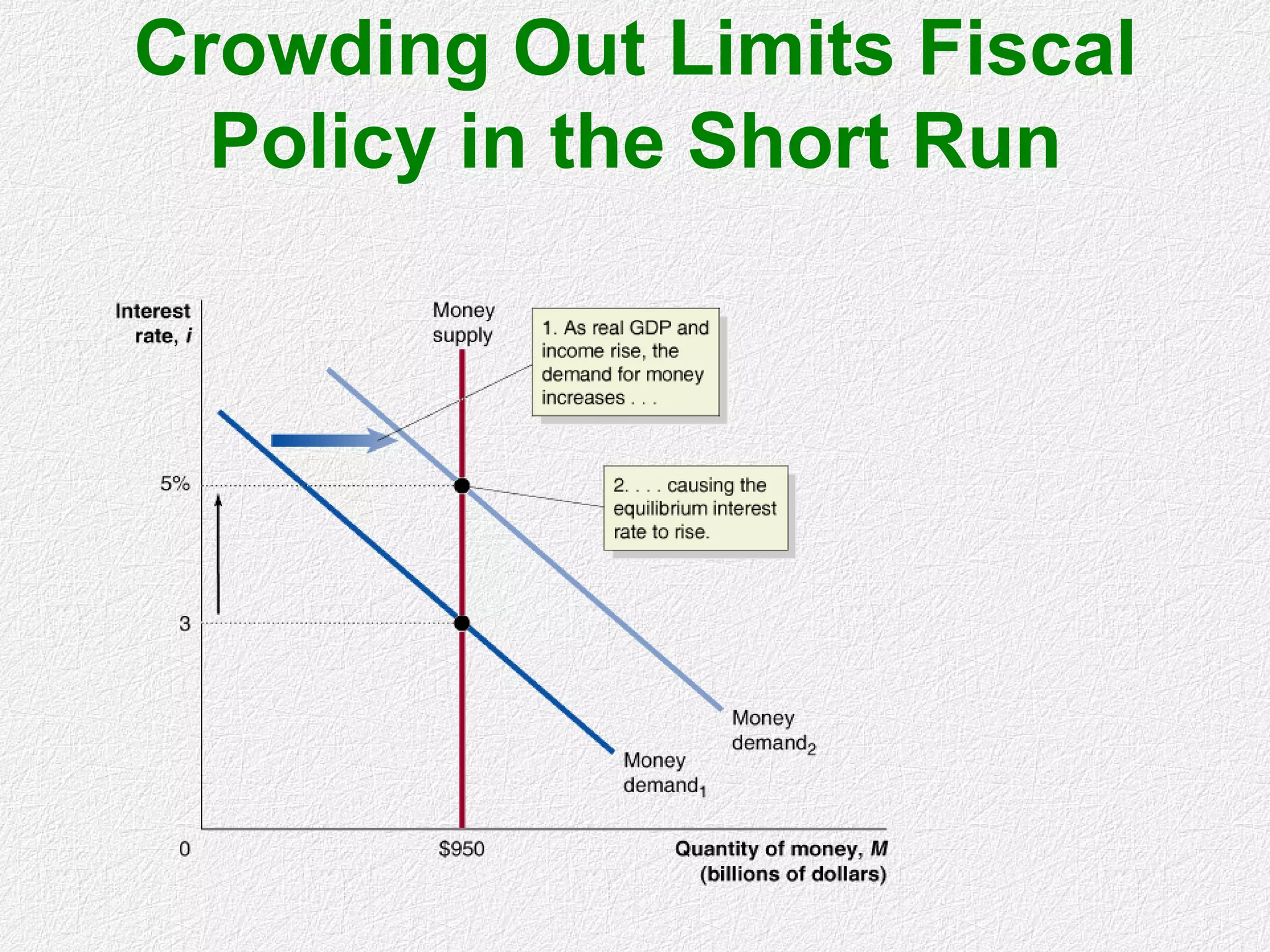

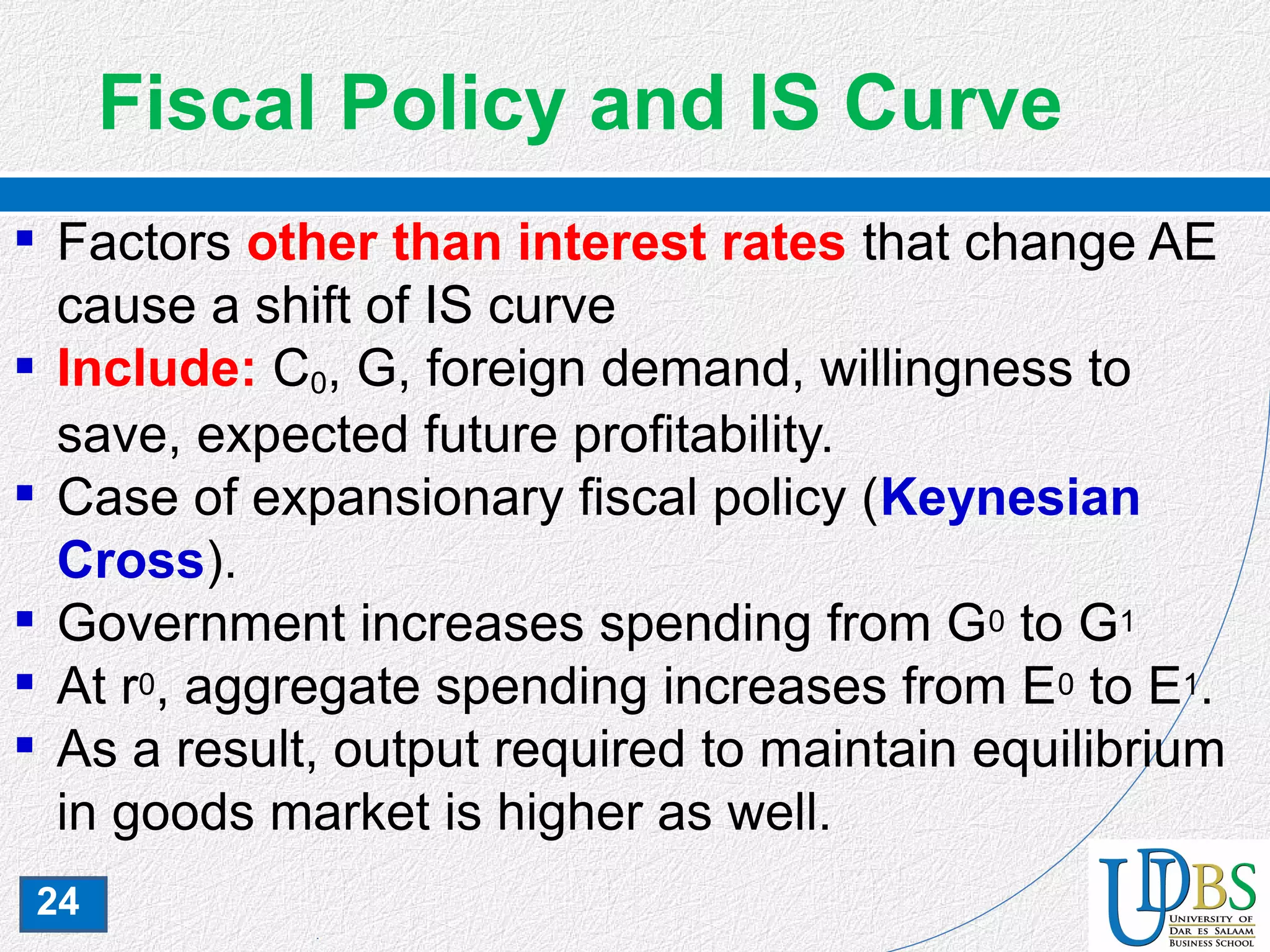


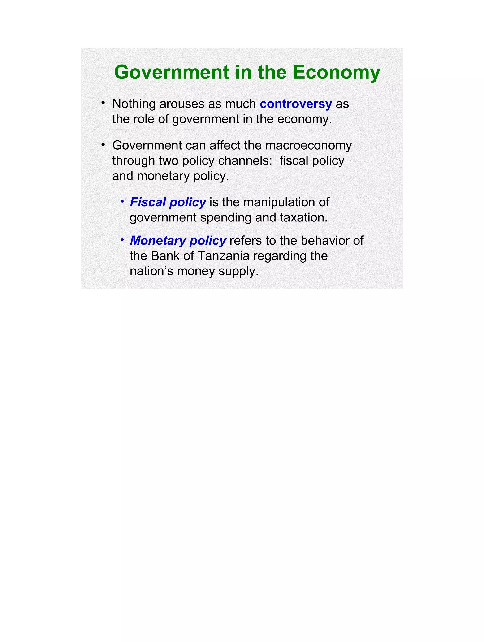
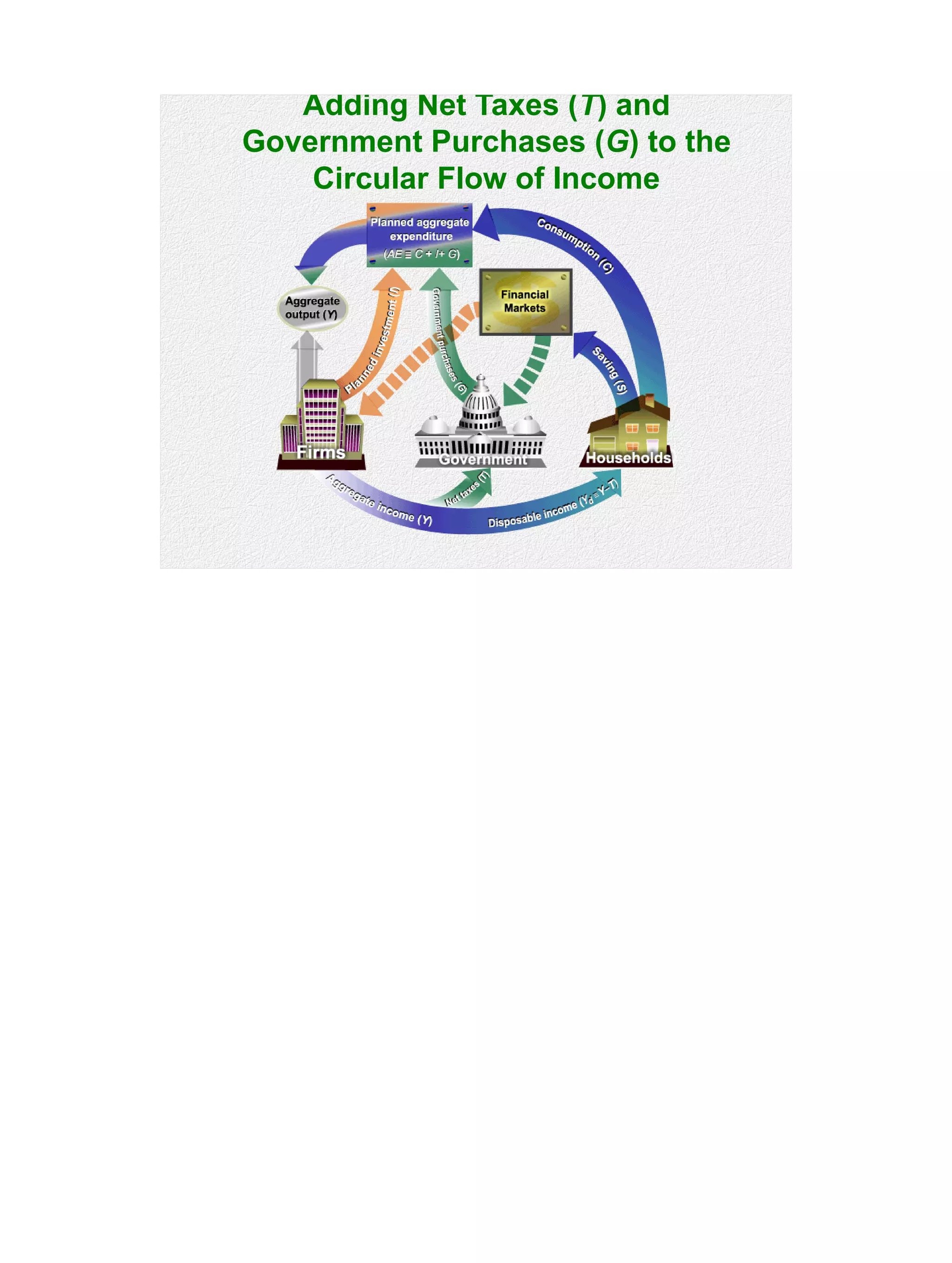
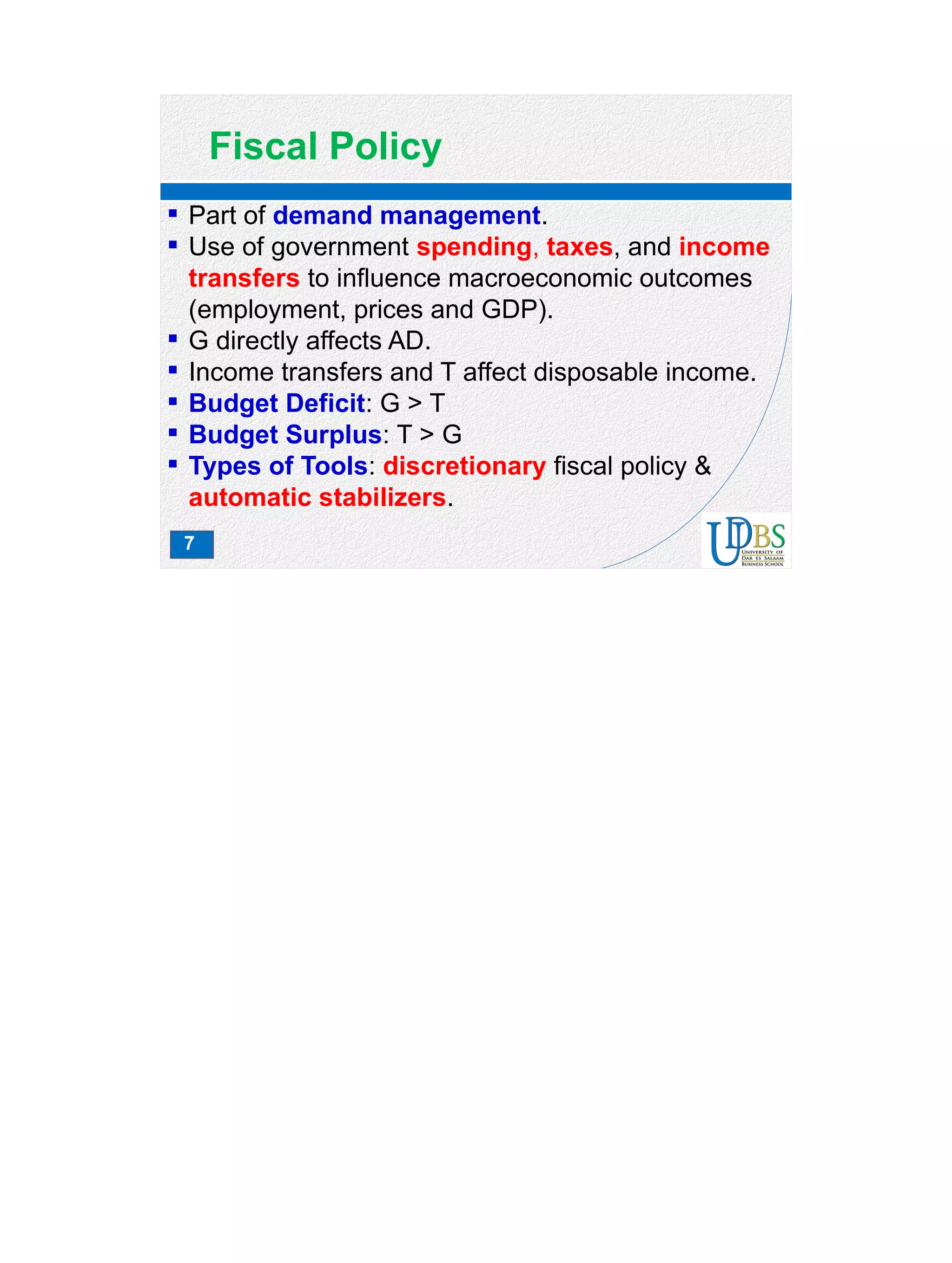
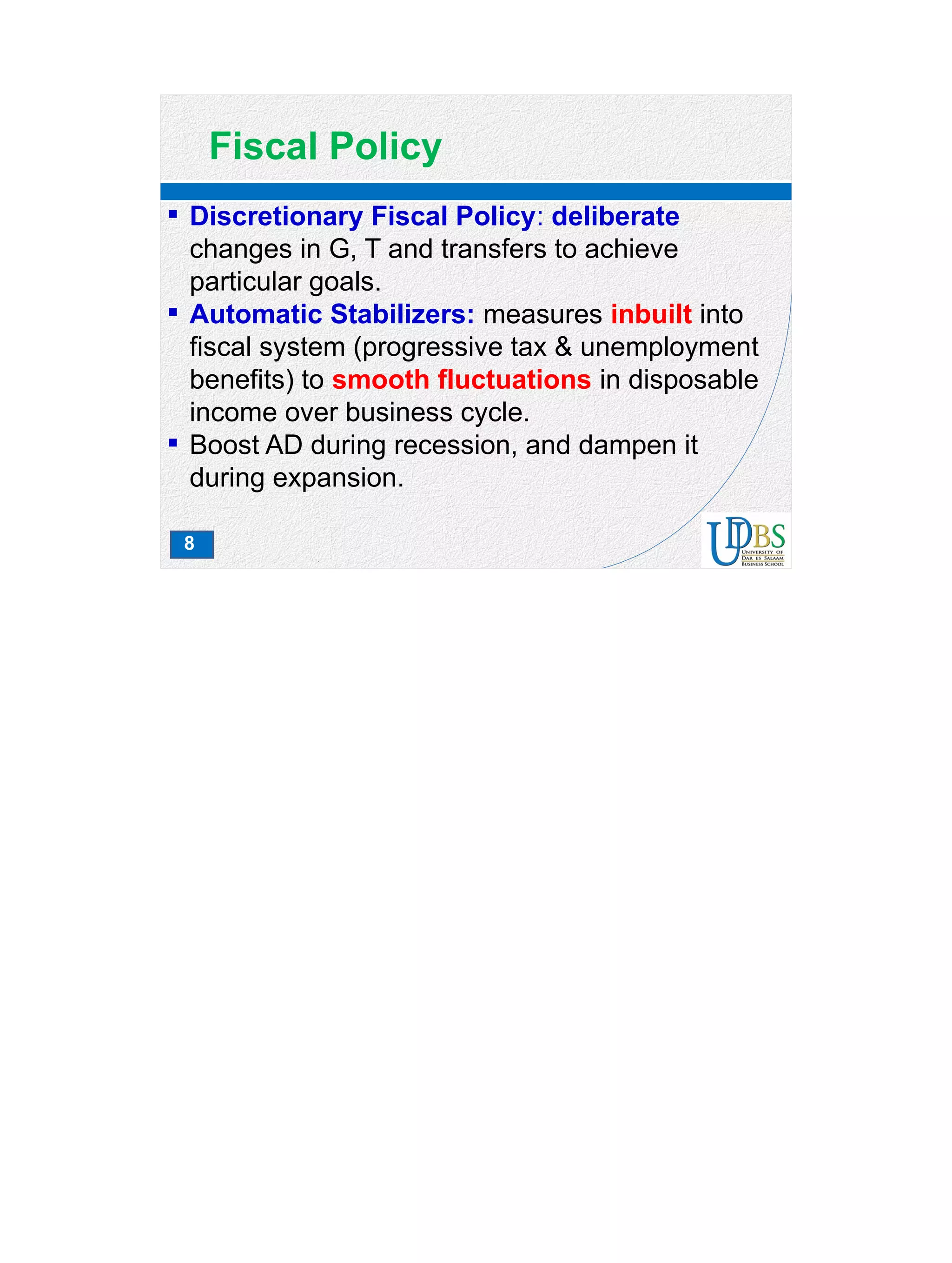


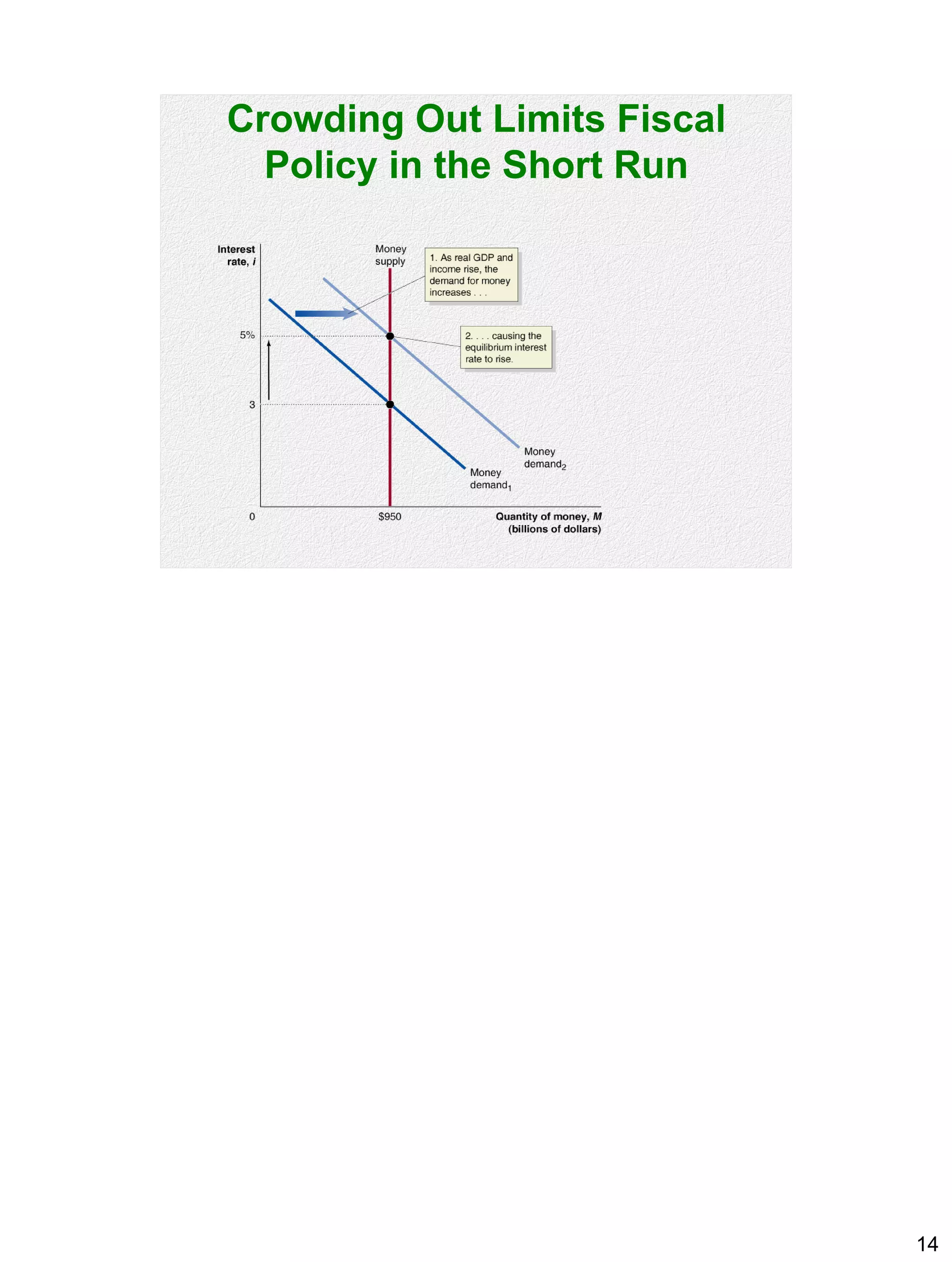
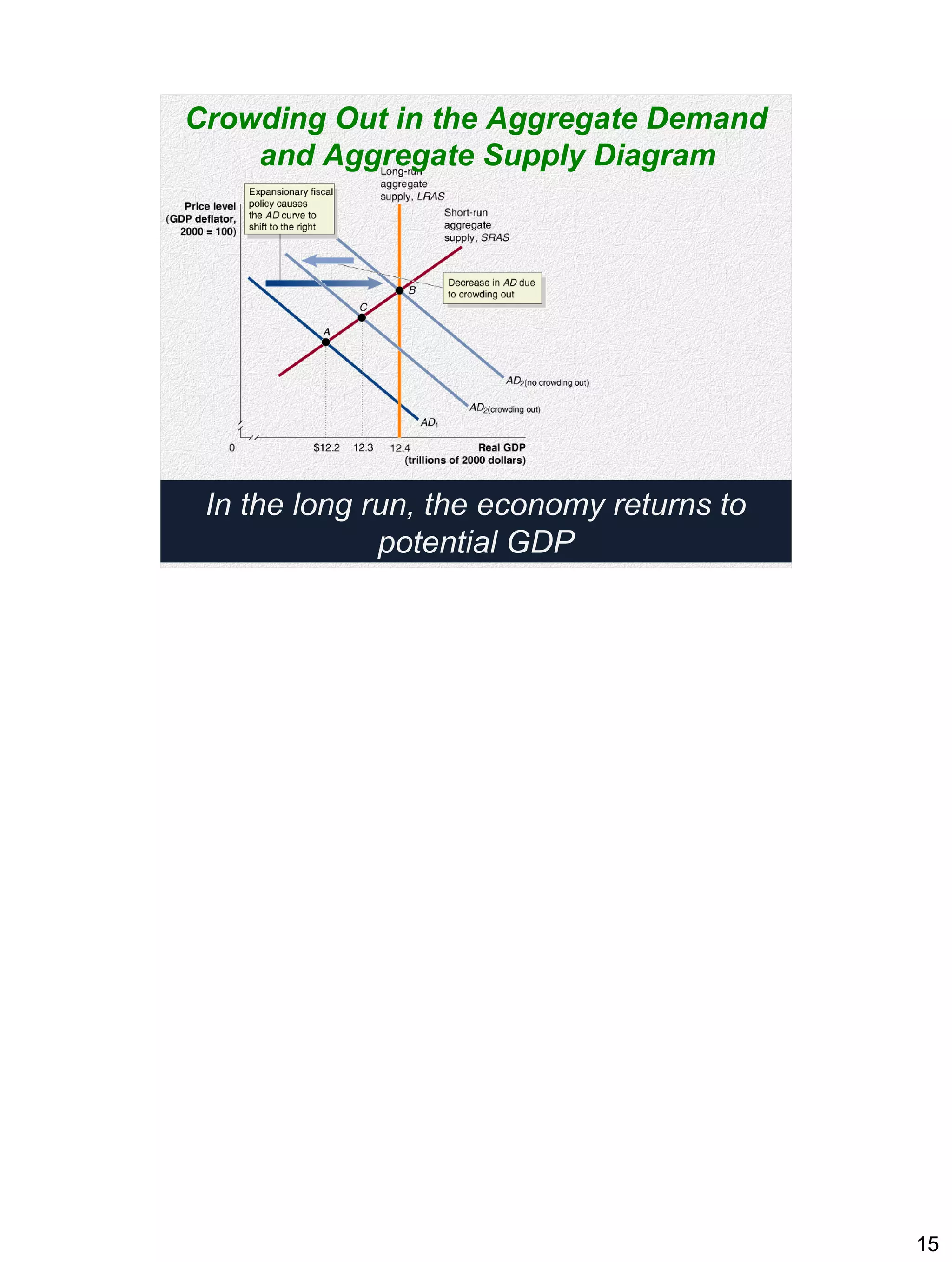


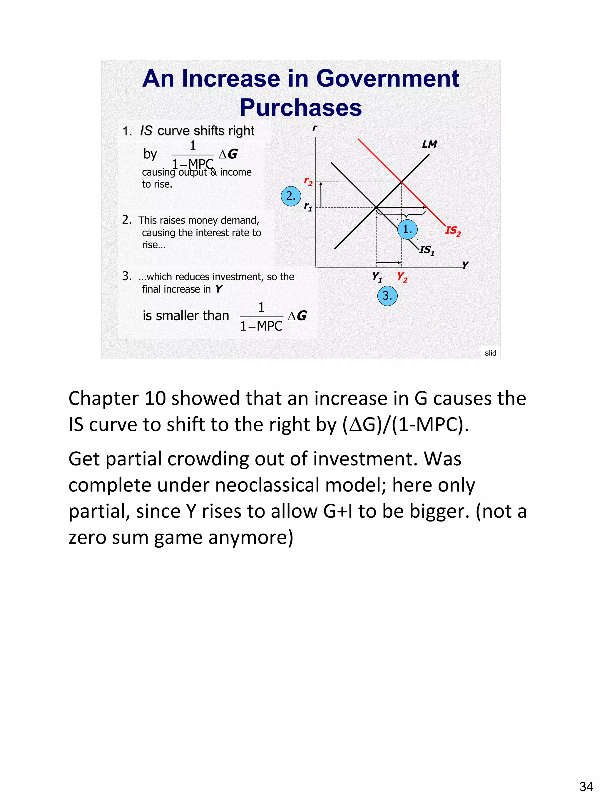


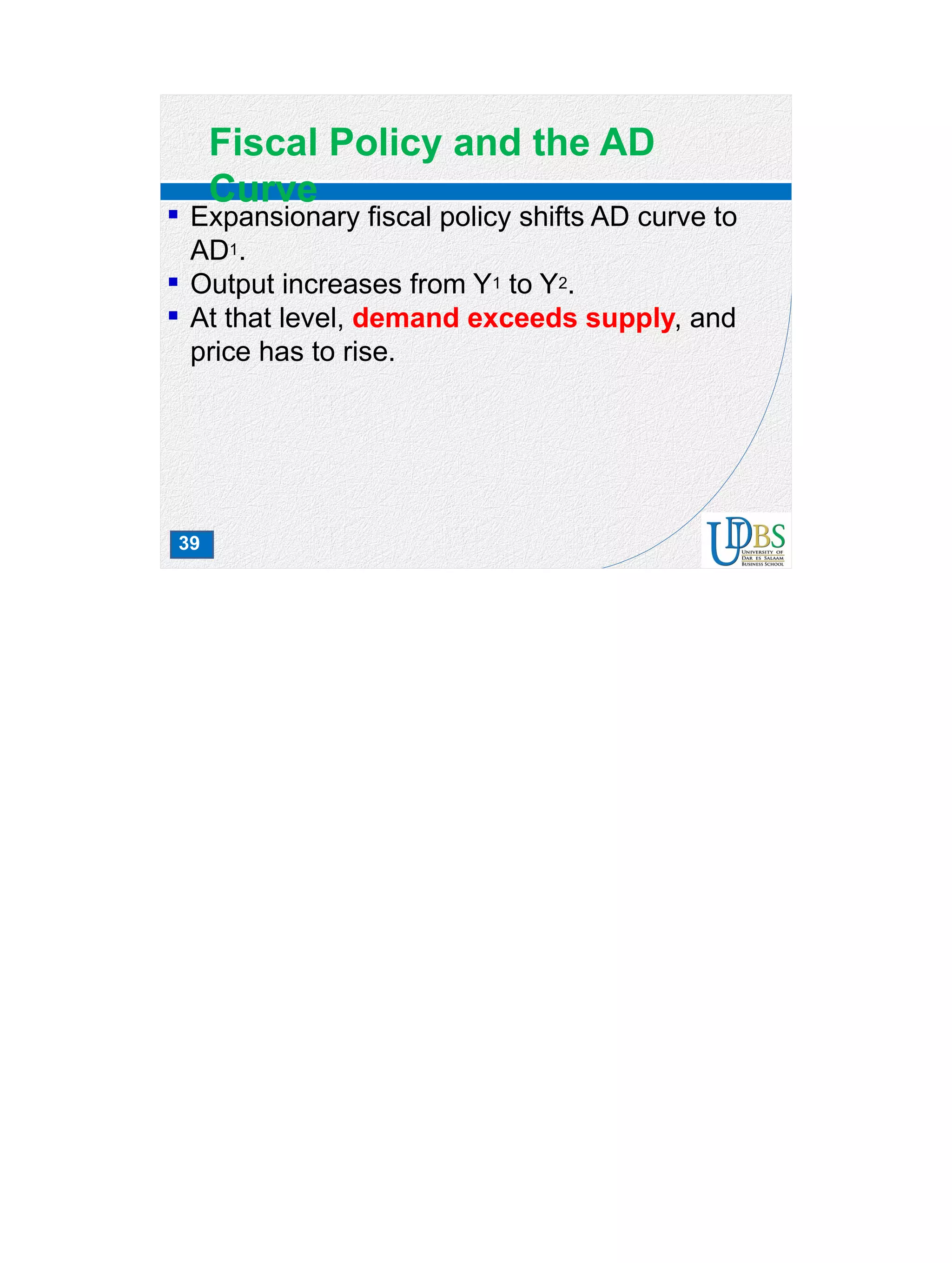


This document discusses fiscal policy and the role of government in the economy. It explains that government can influence the macroeconomy through fiscal policy, which is the manipulation of government spending and taxes. Expansionary fiscal policy, such as increasing government spending, can shift the aggregate demand curve to the right, leading to higher output and income in the short run. However, higher output may also lead to inflation as demand for money increases.


![Presentation1[1].pptxszdsdsdsffsdfsfsdffsf](https://cdn.slidesharecdn.com/ss_thumbnails/presentation11-240805174921-9ada2eb3-thumbnail.jpg?width=640&height=640&fit=bounds)


