Gaussian Multiplicative Chaos (GMC) is a canonical construction that turns a sufficiently regular Gaussian field into a random measure of the form exp (γX(x)) dx,where X is a log-correlated Gaussian field. The theory originates in the work of Kahane on multiplicative chaos and random measures [1], and has since evolved into a central tool at the intersection of probability theory, mathematical physics, and fractal geometry

1. Gaussian Multiplicative Chaos:
A Survey of Theory, Structure, and Applications
December 11, 2025
Contents
1 Introduction 2
2 Gaussian log-correlated fields 3
2.1 General set-up . . . . . . . . . . . . . . . . . . . . . . . . . . . . . . . . . . . . . . . 3
2.2 Examples . . . . . . . . . . . . . . . . . . . . . . . . . . . . . . . . . . . . . . . . . . 3
3 Construction of Gaussian multiplicative chaos 4
3.1 Regularization and renormalization . . . . . . . . . . . . . . . . . . . . . . . . . . . . 4
3.2 Kahane’s multiplicative chaos . . . . . . . . . . . . . . . . . . . . . . . . . . . . . . . 5
3.3 Shamov’s characterization and universality . . . . . . . . . . . . . . . . . . . . . . . 5
3.4 A schematic diagram of the construction . . . . . . . . . . . . . . . . . . . . . . . . . 5
4 Phase diagram: subcritical, critical, and supercritical regimes 5
4.1 Critical value and normalization . . . . . . . . . . . . . . . . . . . . . . . . . . . . . 5
4.2 Subcritical regime . . . . . . . . . . . . . . . . . . . . . . . . . . . . . . . . . . . . . 5
4.3 Critical regime . . . . . . . . . . . . . . . . . . . . . . . . . . . . . . . . . . . . . . . 6
4.4 Supercritical regime and atomic chaos . . . . . . . . . . . . . . . . . . . . . . . . . . 6
4.5 Summary table of regimes . . . . . . . . . . . . . . . . . . . . . . . . . . . . . . . . . 6
4.6 A schematic phase diagram . . . . . . . . . . . . . . . . . . . . . . . . . . . . . . . . 7
5 Structural and multifractal properties 7
5.1 Multifractality and thick points . . . . . . . . . . . . . . . . . . . . . . . . . . . . . . 7
5.2 Moment scaling and multifractal spectrum . . . . . . . . . . . . . . . . . . . . . . . . 7
5.3 Star-scale invariance . . . . . . . . . . . . . . . . . . . . . . . . . . . . . . . . . . . . 8
5.4 A schematic star-scale invariance diagram . . . . . . . . . . . . . . . . . . . . . . . . 8
5.5 Universality and stability . . . . . . . . . . . . . . . . . . . . . . . . . . . . . . . . . 8
6 GMC in probability and analysis 8
6.1 Extremes of log-correlated fields . . . . . . . . . . . . . . . . . . . . . . . . . . . . . 8
6.2 Liouville Brownian motion . . . . . . . . . . . . . . . . . . . . . . . . . . . . . . . . . 9
6.3 Fractal geometry and Hausdorff measures . . . . . . . . . . . . . . . . . . . . . . . . 9
1

2. 7 GMC in mathematical physics 10
7.1 Liouville quantum gravity . . . . . . . . . . . . . . . . . . . . . . . . . . . . . . . . . 10
7.2 KPZ relation . . . . . . . . . . . . . . . . . . . . . . . . . . . . . . . . . . . . . . . . 10
7.3 Liouville conformal field theory . . . . . . . . . . . . . . . . . . . . . . . . . . . . . . 10
8 GMC, stochastic PDEs, and KPZ-type structures 11
8.1 Stochastic heat equation and KPZ . . . . . . . . . . . . . . . . . . . . . . . . . . . . 11
8.2 SPDE-based approximations to GMC . . . . . . . . . . . . . . . . . . . . . . . . . . 11
8.3 Renormalization and regularity structures . . . . . . . . . . . . . . . . . . . . . . . . 12
8.4 A schematic SPDE–GMC diagram . . . . . . . . . . . . . . . . . . . . . . . . . . . . 12
9 GMC, Markov random fields, and exponential tilts 12
9.1 Gaussian Markov random fields and log-correlated limits . . . . . . . . . . . . . . . . 12
9.2 Exponential tilts and Gibbs measures . . . . . . . . . . . . . . . . . . . . . . . . . . 12
9.3 DLR equations and infinite-volume limits . . . . . . . . . . . . . . . . . . . . . . . . 13
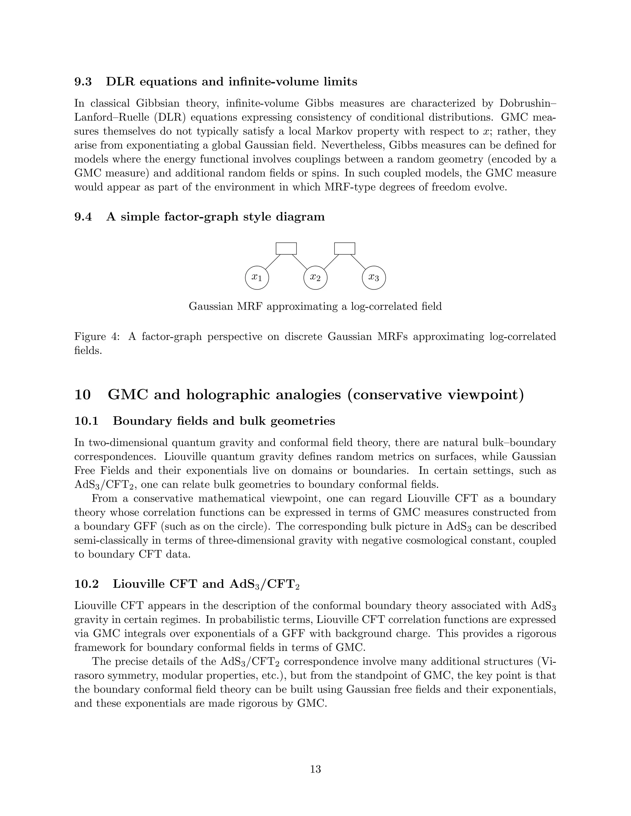
9.4 A simple factor-graph style diagram . . . . . . . . . . . . . . . . . . . . . . . . . . . 13
10 GMC and holographic analogies (conservative viewpoint) 13
10.1 Boundary fields and bulk geometries . . . . . . . . . . . . . . . . . . . . . . . . . . . 13
10.2 Liouville CFT and AdS3/CFT2 . . . . . . . . . . . . . . . . . . . . . . . . . . . . . . 13
10.3 Boundary random measures and bulk observables . . . . . . . . . . . . . . . . . . . . 14
10.4 A schematic holographic diagram . . . . . . . . . . . . . . . . . . . . . . . . . . . . . 14
11 Random matrices and analytic number theory 14
11.1 Characteristic polynomials of random unitary matrices . . . . . . . . . . . . . . . . . 14
11.2 Random Hermitian matrices . . . . . . . . . . . . . . . . . . . . . . . . . . . . . . . . 14
11.3 Riemann zeta function . . . . . . . . . . . . . . . . . . . . . . . . . . . . . . . . . . . 14
12 GMC in turbulence and finance 15
12.1 Kolmogorov–Obukhov model and intermittency . . . . . . . . . . . . . . . . . . . . . 15
12.2 Financial time series and volatility . . . . . . . . . . . . . . . . . . . . . . . . . . . . 15
13 Open problems and further directions 15
1 Introduction
Gaussian Multiplicative Chaos (GMC) is a canonical construction that turns a sufficiently regular
Gaussian field into a random measure of the form
eγX(x)
dx,
where X is a log-correlated Gaussian field. The theory originates in the work of Kahane on
multiplicative chaos and random measures [1], and has since evolved into a central tool at the
intersection of probability theory, mathematical physics, and fractal geometry.
The basic phenomenon is that many models in analysis and physics involve Gaussian fields
whose covariance diverges logarithmically at short distances. These fields do not admit pointwise
values. Nevertheless, one can regularize them and consider exponentials of the form
exp
γXε(x) −
γ2
2
E[Xε(x)2
]
,
2

3. and then study the limit as the regularization scale ε → 0. When this limit exists and is non-trivial,
one obtains a random measure Mγ which is highly singular and exhibits multifractal behavior.
Gaussian multiplicative chaos now appears in a wide range of contexts: Liouville quantum
gravity and Liouville conformal field theory, random planar maps and KPZ-type relations, random
matrix theory, the Riemann zeta function, turbulence and intermittency, and models of multi-scale
volatility. There is also a deep structural connection with multiplicative cascades and branching
random walks.
The purpose of this article is to give a survey-style overview of:
• the construction and phase diagram of Gaussian multiplicative chaos,
• the main structural and multifractal properties of GMC measures,
• applications in probability, analysis, and mathematical physics,
• connections to stochastic partial differential equations (SPDEs), Markov random fields (MRFs),
and conservative holographic analogies (such as the relationship between Liouville CFT and
AdS3/CFT2).
We emphasize a unified probabilistic viewpoint, following the foundational works of Kahane
[1], Robert–Vargas [2], Shamov [3], and the detailed survey of Rhodes–Vargas [4]. Our aim is to
provide a readable but technically informed introduction suitable for researchers with background
in probability or mathematical physics.
2 Gaussian log-correlated fields
2.1 General set-up
Let D ⊂ Rd be a bounded domain and let X be a centered Gaussian field indexed by D (more
precisely, a Gaussian random distribution on D). We say that X is log-correlated if its covariance
kernel has a logarithmic singularity along the diagonal. A canonical form is
E[X(x)X(y)] = log
1
|x − y|
+ g(x, y), (2.1)
for x, y in D, where g is a bounded, continuous function near the diagonal. This structure appears
in many models, including the two-dimensional Gaussian Free Field (GFF), one-dimensional 1/f
noises, and scaling limits of branching random walks and random matrix characteristic polynomials.
Since the covariance diverges when x → y, X is typically only a generalized function. In
particular, X(x) is not defined pointwise but only when tested against smooth functions. This
motivates the regularization approach.
2.2 Examples
Two-dimensional Gaussian Free Field. On a simply connected domain D ⊂ R2 with Dirichlet
boundary conditions, the Gaussian Free Field h is a centered Gaussian process indexed by test
functions f with covariance
E[h(f)h(g)] =
Z
D
Z
D
f(x)GD(x, y)g(y) dx dy,
3

4. where GD is the Green’s function of the Laplacian on D. Near the diagonal, one has
GD(x, y) = −
1
2π
log |x − y| + H(x, y),
with H continuous. Thus, if one attempts to think of h(x) informally, its covariance behaves like a
logarithm at short distances, and h is a prototypical log-correlated field in dimension two.
Circle GFF and Fourier series. On the unit circle T, one can consider the random trigono-
metric series
X(θ) =
∞
X
n=1
1
√
n
(an cos(nθ) + bn sin(nθ)) ,
where (an, bn) are i.i.d. standard Gaussian pairs. This formal series defines a log-correlated Gaussian
distribution on T, with covariance behaving like − log |eiθ − eiθ′
| near the diagonal.
Random matrix characteristic polynomials. For a Haar-distributed unitary matrix U, one
can define
XN (θ) := log | det(1 − e−iθ
U)|,
with a suitable choice of branch. After centering and rescaling, these processes converge in distri-
bution as N → ∞ to a log-correlated Gaussian field on the circle. This is a remarkable connection
between random matrix theory and the GMC universality class, studied in [8, 9, 10].
3 Construction of Gaussian multiplicative chaos
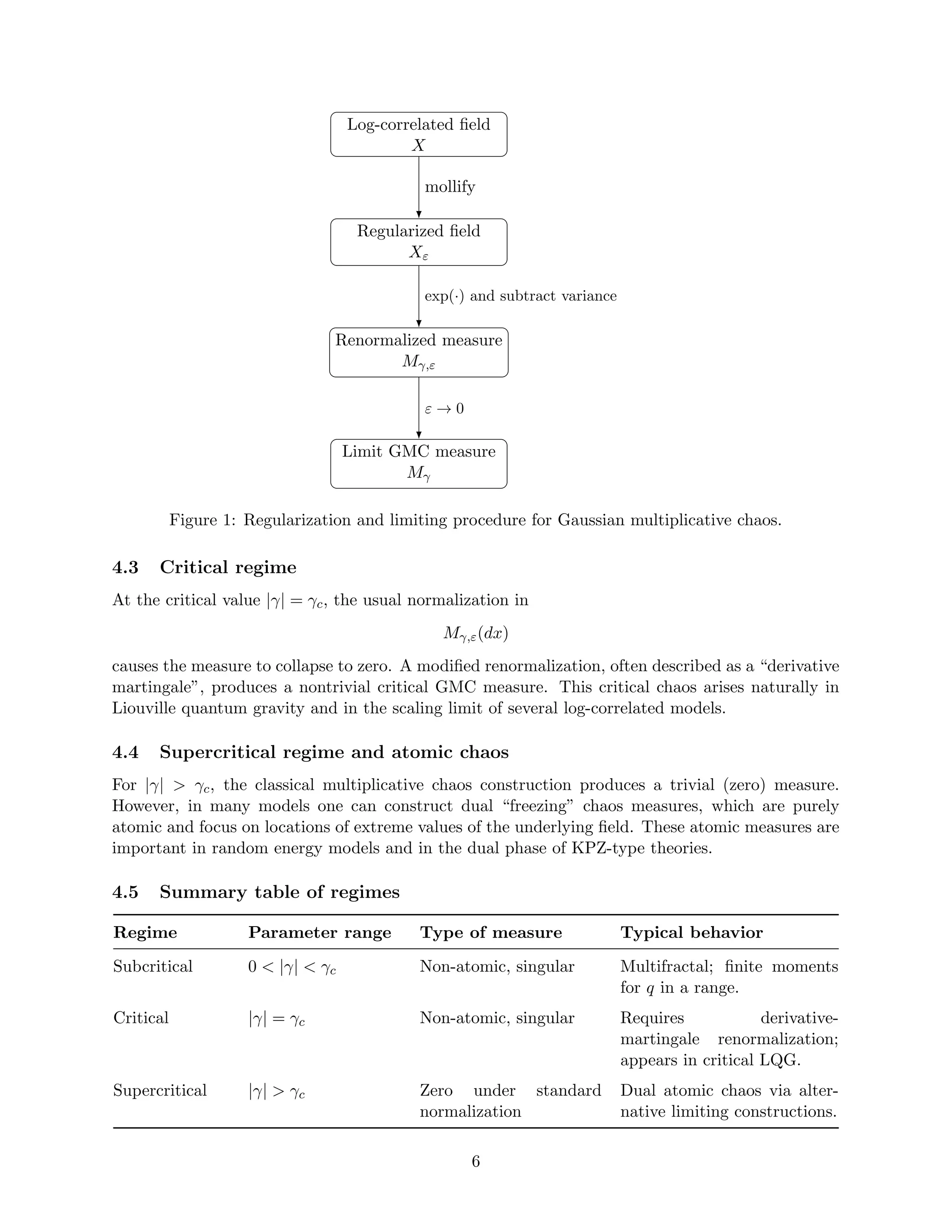
3.1 Regularization and renormalization
Let X be a log-correlated Gaussian field on D with covariance of the form (2.1). In order to define
the exponential measure formally given by eγX(x) dx, we consider a family of smooth approximations
(Xε)ε0, for example
Xε(x) := (X ∗ ρε)(x),
where ρε is a mollifier at scale ε. For each ε 0, Xε is a smooth Gaussian field, and the object
exp γXε(x)
is well defined pointwise.
However, as ε → 0, the variance E[Xε(x)2] diverges like log(1/ε). The key renormalization is
to subtract the variance at the exponent level. For γ ∈ R, define the random measures
Mγ,ε(dx) := exp
γXε(x) −
γ2
2
E[Xε(x)2
]
dx. (3.1)
The subtraction of γ2
2 E[Xε(x)2] ensures that E[Mγ,ε(A)] remains of constant order as ε → 0 for
reasonable sets A ⊂ D.
4

5. 3.2 Kahane’s multiplicative chaos
Kahane introduced the notion of multiplicative chaos in a fairly general setting involving random
measures built from (possibly non-Gaussian) independently scattered noise [1]. In the Gaussian
case, his approach yields existence and non-triviality results for Mγ,ε in a range of parameters γ.
A fundamental result is that when |γ| is smaller than a critical parameter γc (depending on
the dimension and the covariance), the measures Mγ,ε converge (along suitable subsequences) to
a non-degenerate limit Mγ in the weak topology of measures. This limit is called the Gaussian
multiplicative chaos associated with the field X and parameter γ.
3.3 Shamov’s characterization and universality
Shamov [3] developed an intrinsic, approximation-free definition of subcritical Gaussian multiplica-
tive chaos. Let X be a centered Gaussian field on a measure space (T, µ) with covariance kernel
K. The law of X can be viewed as a Gaussian measure on a suitable Hilbert space. A random
measure M on T is called a (subcritical) Gaussian multiplicative chaos associated with X if:
(i) E[M(A)] = µ(A) for all measurable A ⊂ T,
(ii) for every deterministic ξ in the Cameron–Martin space of X, the shift property holds
M(X + ξ, dt) = eξ(t)
M(X, dt) a.s.
Under mild conditions, this characterizes the law of M uniquely in the subcritical regime. In
particular, any sequence of approximations (Xε) which converges to X in the Gaussian sense and
satisfies basic regularity conditions will generate the same limiting GMC measure (up to determin-
istic factors). This universality is a key reason why GMC appears in so many different models.
3.4 A schematic diagram of the construction
4 Phase diagram: subcritical, critical, and supercritical regimes
4.1 Critical value and normalization
For log-correlated fields in dimension d, the critical parameter is typically
γc =
√
2d
under a standard normalization of the covariance. For |γ| γc, the GMC is called subcritical and
yields a non-degenerate random measure. At γ = γc, a different renormalization scheme is needed
to obtain a non-trivial limit (critical GMC). For |γ| γc, the standard normalization leads to
trivial (zero) measures, although dual, purely atomic chaos measures can be constructed in various
ways.
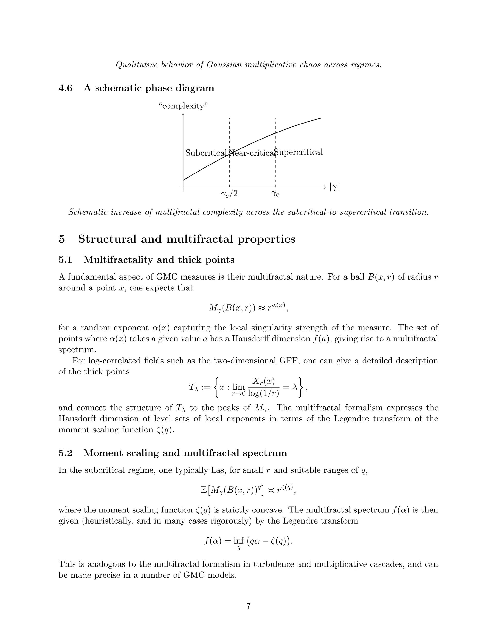
4.2 Subcritical regime
In the subcritical phase 0 |γ| γc, the random measure Mγ is almost surely non-atomic and
singular with respect to the reference measure µ. It exhibits multifractal behavior: local masses
satisfy
Mγ(B(x, r)) ≈ rα(x)
,
with a random exponent α(x) having a nontrivial distribution related to thick points of the Gaussian
field.
5

6. Log-correlated field
X
Regularized field
Xε
Renormalized measure
Mγ,ε
Limit GMC measure
Mγ
mollify
exp(·) and subtract variance
ε → 0
Figure 1: Regularization and limiting procedure for Gaussian multiplicative chaos.
4.3 Critical regime
At the critical value |γ| = γc, the usual normalization in
Mγ,ε(dx)
causes the measure to collapse to zero. A modified renormalization, often described as a “derivative
martingale”, produces a nontrivial critical GMC measure. This critical chaos arises naturally in
Liouville quantum gravity and in the scaling limit of several log-correlated models.
4.4 Supercritical regime and atomic chaos
For |γ| γc, the classical multiplicative chaos construction produces a trivial (zero) measure.
However, in many models one can construct dual “freezing” chaos measures, which are purely
atomic and focus on locations of extreme values of the underlying field. These atomic measures are
important in random energy models and in the dual phase of KPZ-type theories.
4.5 Summary table of regimes
Regime Parameter range Type of measure Typical behavior
Subcritical 0 |γ| γc Non-atomic, singular Multifractal; finite moments
for q in a range.
Critical |γ| = γc Non-atomic, singular Requires derivative-
martingale renormalization;
appears in critical LQG.
Supercritical |γ| γc Zero under standard
normalization
Dual atomic chaos via alter-
native limiting constructions.
6

7. Qualitative behavior of Gaussian multiplicative chaos across regimes.
4.6 A schematic phase diagram
|γ|
“complexity”
γc/2 γc
SubcriticalNear-critical
Supercritical
Schematic increase of multifractal complexity across the subcritical-to-supercritical transition.
5 Structural and multifractal properties
5.1 Multifractality and thick points
A fundamental aspect of GMC measures is their multifractal nature. For a ball B(x, r) of radius r
around a point x, one expects that
Mγ(B(x, r)) ≈ rα(x)
,
for a random exponent α(x) capturing the local singularity strength of the measure. The set of
points where α(x) takes a given value a has a Hausdorff dimension f(a), giving rise to a multifractal
spectrum.
For log-correlated fields such as the two-dimensional GFF, one can give a detailed description
of the thick points
Tλ :=
x : lim
r→0
Xr(x)
log(1/r)
= λ
,
and connect the structure of Tλ to the peaks of Mγ. The multifractal formalism expresses the
Hausdorff dimension of level sets of local exponents in terms of the Legendre transform of the
moment scaling function ζ(q).
5.2 Moment scaling and multifractal spectrum
In the subcritical regime, one typically has, for small r and suitable ranges of q,
E
Mγ(B(x, r))q
≍ rζ(q)
,
where the moment scaling function ζ(q) is strictly concave. The multifractal spectrum f(α) is then
given (heuristically, and in many cases rigorously) by the Legendre transform
f(α) = inf
q
qα − ζ(q)
.
This is analogous to the multifractal formalism in turbulence and multiplicative cascades, and can
be made precise in a number of GMC models.
7

8. 5.3 Star-scale invariance
GMC measures are examples of ∗-scale invariant random measures. Informally, this means that if
one zooms in by a factor r, the measure decomposes into a random multiplicative factor determined
by the increment of the field, times an independent copy of the original measure. This property
is shared with multiplicative cascades and plays a key role in the connection between discrete and
continuous models.
More precisely, in many settings one has a relation of the form
Mγ(dx)
d
=
Z
exp
γYr(x) − γ2
2 E[Yr(x)2
]
M(r)
γ (dx),
where Yr is an appropriate Gaussian increment at scale r, and M
(r)
γ is a rescaled version of Mγ,
independent of Yr. Such relations link GMC to canonical models of multiplicative cascades and to
the theory of log-infinitely divisible random measures.
5.4 A schematic star-scale invariance diagram
Mγ
global measure
M
(r)
γ
rescaled copy
eγYr−γ2
2
EY 2
r
multiplicative factor
zoom in field increment
))
Mγ
d
= (multiplicative factor) × M
(r)
γ
Figure 2: Informal star-scale invariance structure of GMC measures.
5.5 Universality and stability
Shamov’s characterization ensures that subcritical GMC measures are stable under changes of ap-
proximation. For example, mollification by different kernels, spectral truncation, or circle-averaging
procedures all yield the same limiting measure, provided the approximations converge to the same
Gaussian field. This universality is a key reason why GMC appears in so many different models: as
long as the underlying field is log-correlated and the covariance structure is compatible, the limiting
measure is essentially unique.
Moreover, many quantitative properties of GMC (such as moment bounds, tail behavior, and
thick point geometry) depend only on a small number of parameters (e.g. the variance normalization
of X and the dimension d), reinforcing the idea that GMC defines a robust universality class for
multifractal random measures.
6 GMC in probability and analysis
6.1 Extremes of log-correlated fields
The maximum of a log-correlated Gaussian field on a bounded domain exhibits non-trivial fluctu-
ations. A recurring theme is that the extreme values of X are closely related to the peaks of the
8

9. GMC measure Mγ. In many models, the asymptotic distribution of the centered maximum can be
expressed in terms of the limit of certain functionals of Mγ, and the tail behavior is influenced by
the multifractal structure.
For instance, consider a log-correlated field X on a domain D and define
MN := max
x∈DN
X(x),
where DN is a discrete mesh approximating D at scale N−1. Under appropriate normalization,
MN converges in law to a randomly shifted Gumbel distribution. The shift is often expressed in
terms of a derivative-type chaos or related limit of GMC functionals. This picture is well developed
for branching Brownian motion and branching random walks, and analogous results exist for the
2D GFF and for characteristic polynomials of random matrices.
The link between extremes and GMC is conceptually natural: the most singular points of Mγ
correspond to locations where X takes unusually large values. Thus, understanding the geometry
of thick points and the multifractal spectrum of Mγ informs the asymptotic behavior of extremes.
6.2 Liouville Brownian motion
Given a GMC measure Mγ on a domain D, one can define a time-change of standard Brownian
motion using Mγ as a speed measure. Let (Bt)t≥0 be a Brownian motion on D (with reflection or
absorption at the boundary). Define the additive functional
At =
Z t
0
exp
γX(Bs) − γ2
2 E[X(Bs)2
]
ds
in a suitable regularized sense, or more abstractly,
At =
Z t
0
f(Bs) ds with f dx = Mγ(dx).
The inverse time-change
τu = inf{t ≥ 0 : At u}
defines a new process
Zu = Bτu ,
known as Liouville Brownian motion. Intuitively, Z is Brownian motion in the random geometry
encoded by the Liouville measure Mγ. This construction provides a probabilistic model for diffusion
on Liouville quantum gravity surfaces and is closely related to Dirichlet form techniques and time-
change theory.
6.3 Fractal geometry and Hausdorff measures
GMC is closely connected with the theory of random fractals and Hausdorff measures. In many
cases, one can regard Mγ as a random density that, when combined with deterministic or random
metrics, gives rise to natural random Hausdorff measures on fractal sets. For example, if d(x, y) is
a metric on D (possibly random), one can define a Hausdorff measure with gauge function modified
by the local density of Mγ. The multifractal formalism for Mγ then provides detailed information
about the local dimensions and scaling properties of such measures.
From a technical standpoint, tools from potential theory, capacity, and Frostman-type lemmas
are often used together with GMC to obtain lower and upper bounds on Hausdorff dimensions of
random sets. This interplay has been particularly fruitful in the study of level sets and thick points
of GFF-type fields.
9

10. 7 GMC in mathematical physics
7.1 Liouville quantum gravity
Liouville quantum gravity (LQG) is a probabilistic model of random two-dimensional geometry. In
the original physics literature, it arises from the Liouville action for a scalar field ϕ coupled to the
metric on a 2D surface. Formally, the volume form of the random metric can be written as
eγϕ(z)
dz,
where ϕ is essentially a Gaussian Free Field. The measure theory of LQG thus rests on giving a
meaning to these exponentials, which is precisely what GMC provides.
Duplantier and Sheffield [5] formulated LQG in probabilistic terms and established the KPZ
relation connecting Euclidean and quantum fractal dimensions. The Liouville measure on a planar
domain is, by definition, the GMC measure associated with a 2D GFF and a coupling constant γ
in a certain range. This random measure describes the area element of the random surface.
LQG also arises as the scaling limit of random planar maps. Various ensembles of random
triangulations and quadrangulations, when rescaled appropriately, converge to continuum random
surfaces whose area measure is described by Liouville GMC. This link between discrete combina-
torial models and continuum random geometry is a major success of the GMC framework.
7.2 KPZ relation
The KPZ relation is a quadratic transformation linking the Euclidean dimension of a fractal set
and its dimension with respect to the LQG measure. If a set K has Euclidean Hausdorff dimension
dE, then its Liouville (or “quantum”) dimension dQ is given by an explicit function
dE =
γ2
4
d2
Q +
1 −
γ2
4
dQ.
This relation was conjectured in the physics literature and proved rigorously in [5, 6]. GMC plays
a central role in the proof, as the Liouville measure determines the quantum geometry in which the
fractal dimension is measured.
Practically, the KPZ relation allows one to transfer dimension estimates between the Euclidean
geometry of subsets of the plane and their geometry in the random metric induced by LQG. This
has been used to analyze the fractal structure of interfaces, geodesics, and other geometric objects
in random planar maps and in continuum LQG.
7.3 Liouville conformal field theory
Liouville conformal field theory (LCFT) is a non-rational conformal field theory whose correlation
functions can be expressed in terms of GMC measures. Expectation values of vertex operators
eαϕ(z) can be written as integrals involving powers of GMC measures.
Remy [7] used this connection to prove the Fyodorov–Bouchaud formula, which gives the exact
distribution of the total mass of a subcritical GMC measure on the unit circle. The argument
proceeds by relating negative moments of the total mass to Liouville CFT correlation functions
and using BPZ-type differential equations to identify the law. This provides a striking example in
which ideas from conformal field theory and GMC combine to yield an exact probabilistic result.
More generally, the probabilistic construction of LCFT via GMC offers a rigorous interpretation
of Liouville correlation functions, including the DOZZ structure constants. While many technical
details remain quite intricate, the GMC viewpoint has become standard in mathematical treatments
of LCFT.
10

11. 8 GMC, stochastic PDEs, and KPZ-type structures
8.1 Stochastic heat equation and KPZ
The Kardar–Parisi–Zhang (KPZ) equation in one spatial dimension,
∂th =
1
2
(∂xh)2
+
1
2
∂xxh + ξ,
where ξ is space-time white noise, is formally connected to the stochastic heat equation with
multiplicative noise via the Cole–Hopf transform
Z = eh
.
Formally, Z solves
∂tZ =
1
2
∂xxZ + ξZ.
Solutions to the stochastic heat equation with multiplicative noise exhibit intermittency and multi-
scale fluctuations reminiscent of multiplicative chaos. In particular, the random field Z(t, x) can
have moments that grow super-exponentially in time, and the logarithm of Z can display rough
spatial behavior.
Although the KPZ equation and its universality class differ in structure from the static log-
correlated fields used in GMC, there are conceptual parallels: both involve exponential transforms
of Gaussian-type objects and produce random measures with intermittent peaks. In certain scaling
regimes, asymptotic fields derived from stochastic heat equations and related models have log-
correlated limits, and their exponential transforms can give rise to GMC-type measures.
8.2 SPDE-based approximations to GMC
In some constructions, log-correlated fields can be represented as time-integrals of solutions to
linear SPDEs. For example, one may represent a GFF as an integral over the heat kernel or as the
stationary solution of a suitable stochastic PDE. When such representations are available, they can
be used to construct GMC via SPDE approximations rather than direct spectral or convolutional
regularization.
The general idea is to consider a family of Gaussian fields
XT (x) =
Z T
0
Φt(x) dWt,
where (Φt) is a deterministic family of operators (often involving the heat semigroup) and Wt is a
cylindrical Brownian motion. As T → ∞, XT converges in distribution to a log-correlated field X.
One can then consider the measures
Mγ,T (dx) = exp
γXT (x) − γ2
2 E[XT (x)2
]
dx
and study their convergence to a GMC measure Mγ. This viewpoint connects the GMC construction
to techniques from SPDEs and stochastic quantization.
11

12. 8.3 Renormalization and regularity structures
In the theory of singular stochastic PDEs, renormalization is used to make sense of equations whose
nonlinearities are ill-defined when driven by distributions (rather than functions). A well-known
example is Hairer’s theory of regularity structures. The renormalization procedures in SPDEs often
involve subtracting divergent constants in a way that is reminiscent of the variance subtraction in
GMC. This parallel is conceptual: both theories use renormalization to define nonlinear functionals
of distributions, although the technical frameworks are different.
8.4 A schematic SPDE–GMC diagram
Linear SPDE
(e.g. stochastic heat equation)
Gaussian field XT
(approximate GFF)
GMC measure Mγ,T
time-integral, T → ∞ exp(·), renorm.
Figure 3: Conceptual link between SPDE-based Gaussian fields and GMC measures.
9 GMC, Markov random fields, and exponential tilts
9.1 Gaussian Markov random fields and log-correlated limits
Markov random fields (MRFs) are random fields whose finite-dimensional distributions satisfy con-
ditional independence properties encoded by a graph or a geometry. Gaussian MRFs are Gaussian
fields whose covariance structure and conditional independence properties are determined by a
precision matrix or an elliptic operator.
Discrete approximations of log-correlated fields, such as the discrete Gaussian free field on a
lattice, are Gaussian MRFs. The continuum GFF can be regarded as a scaling limit of these
discrete MRFs. In this sense, GMC measures constructed from log-correlated fields can be viewed
as exponential tilts of measures associated with continuum limits of Gaussian MRFs.
9.2 Exponential tilts and Gibbs measures
In finite dimensions, if X is a Gaussian vector and V (x) is a potential, one can define a Gibbs
measure
µV (dx) ∝ e−V (x)
µ0(dx),
where µ0 is the Gaussian measure. In the context of GMC, one considers exponentials of linear
functionals of X:
exp
γX(x) − γ2
2 E[X(x)2
]
.
Integrating these exponentials with respect to a base measure µ yields the GMC measure. At a
formal level, one can think of GMC as the exponential tilt
dMγ
dµ
(x) = exp
γX(x) − γ2
2 E[X(x)2
]
.
For each realization of X, this defines a density with respect to µ.
12

13. 9.3 DLR equations and infinite-volume limits
In classical Gibbsian theory, infinite-volume Gibbs measures are characterized by Dobrushin–
Lanford–Ruelle (DLR) equations expressing consistency of conditional distributions. GMC mea-
sures themselves do not typically satisfy a local Markov property with respect to x; rather, they
arise from exponentiating a global Gaussian field. Nevertheless, Gibbs measures can be defined for
models where the energy functional involves couplings between a random geometry (encoded by a
GMC measure) and additional random fields or spins. In such coupled models, the GMC measure
would appear as part of the environment in which MRF-type degrees of freedom evolve.
9.4 A simple factor-graph style diagram
x1 x2 x3
Gaussian MRF approximating a log-correlated field
Figure 4: A factor-graph perspective on discrete Gaussian MRFs approximating log-correlated
fields.
10 GMC and holographic analogies (conservative viewpoint)
10.1 Boundary fields and bulk geometries
In two-dimensional quantum gravity and conformal field theory, there are natural bulk–boundary
correspondences. Liouville quantum gravity defines random metrics on surfaces, while Gaussian
Free Fields and their exponentials live on domains or boundaries. In certain settings, such as
AdS3/CFT2, one can relate bulk geometries to boundary conformal fields.
From a conservative mathematical viewpoint, one can regard Liouville CFT as a boundary
theory whose correlation functions can be expressed in terms of GMC measures constructed from
a boundary GFF (such as on the circle). The corresponding bulk picture in AdS3 can be described
semi-classically in terms of three-dimensional gravity with negative cosmological constant, coupled
to boundary CFT data.
10.2 Liouville CFT and AdS3/CFT2
Liouville CFT appears in the description of the conformal boundary theory associated with AdS3
gravity in certain regimes. In probabilistic terms, Liouville CFT correlation functions are expressed
via GMC integrals over exponentials of a GFF with background charge. This provides a rigorous
framework for boundary conformal fields in terms of GMC.
The precise details of the AdS3/CFT2 correspondence involve many additional structures (Vi-
rasoro symmetry, modular properties, etc.), but from the standpoint of GMC, the key point is that
the boundary conformal field theory can be built using Gaussian free fields and their exponentials,
and these exponentials are made rigorous by GMC.
13

14. 10.3 Boundary random measures and bulk observables
One can think of GMC measures on the boundary as encoding random weights that influence bulk
observables. For example, certain gravitational observables in the bulk can be related to insertions
of vertex operators in the boundary theory, whose correlation functions involve GMC. From this
perspective, GMC provides a probabilistic language for the boundary side of a holographic relation,
while the bulk side is described by geometric or gravitational models.
10.4 A schematic holographic diagram
Boundary CFT with GMC
Bulk geometry (e.g. AdS3)
holographic map
Figure 5: Conservative schematic of a bulk–boundary relation: GMC measures on the boundary
enter Liouville CFT, which is related to a bulk gravitational model.
11 Random matrices and analytic number theory
11.1 Characteristic polynomials of random unitary matrices
For the Circular Unitary Ensemble (CUE), the characteristic polynomial
PN (θ) = det(1 − e−iθ
U)
has logarithm XN (θ) = log |PN (θ)| that converges in distribution to a log-correlated Gaussian field
on the circle after suitable centering and normalization. Webb [8] showed that in the L2 regime,
exponentials of XN converge to a GMC measure on the circle, and Nikula–Saksman–Webb [9]
extended this to the L1 phase, establishing convergence for the full subcritical range of γ.
These results link the multifractal structure of characteristic polynomials to GMC and provide
a detailed description of their thick points and extreme values.
11.2 Random Hermitian matrices
Berestycki [10] proved analogous results for a broad class of random Hermitian matrices, showing
that the logarithms of characteristic polynomials converge to log-correlated fields and that their
exponentials converge to GMC measures. This demonstrates the robustness of the GMC description
across random matrix ensembles and supports the universality of log-correlated Gaussian fields in
spectral statistics.
11.3 Riemann zeta function
Fyodorov, Hiary, and Keating conjectured that the maxima of |ζ(1/2 + it)| over intervals behave
like the maxima of log-correlated Gaussian fields. Saksman and Webb [11] proved that, in an
14

15. appropriate mesoscopic scaling regime, the Riemann zeta function on the critical line can be de-
composed into a product of a smooth factor, a diverging scalar factor, and a complex Gaussian
multiplicative chaos. This identifies the “rough” part of zeta fluctuations with GMC and reinforces
the universality of the log-correlated / GMC picture.
These connections between GMC, random matrices, and the zeta function provide a rich inter-
play between probability, spectral theory, and analytic number theory, and continue to be a very
active area of research.
12 GMC in turbulence and finance
12.1 Kolmogorov–Obukhov model and intermittency
Kahane was partly motivated by turbulence when developing multiplicative chaos. The Kolmogorov–
Obukhov model of turbulence assumes a log-normal cascade for energy dissipation across scales.
Robert and Vargas [2] constructed a rigorous version of this model using GMC, providing a mathe-
matically precise turbulence dissipation measure with log-normal statistics. The resulting measures
exhibit intermittency properties similar to those observed experimentally.
In these models, the energy dissipation at scale r is modeled by a multiplicative cascade, which
in the continuum limit becomes a GMC measure over scales or spatial locations. The multifractal
properties of GMC then capture the observed multi-scale variability of turbulence, such as bursts
of high dissipation interspersed with calmer regions.
12.2 Financial time series and volatility
In quantitative finance, log-normal multiplicative cascades have been used to model volatility at
multiple time scales. Bacry and Muzy proposed continuous-time cascade models in which volatility
is driven by a multiplicative cascade across scales. In the continuum limit, these models can be
formulated in terms of Gaussian multiplicative chaos, with the volatility measure at a given time
represented by a GMC measure over scales.
This provides a flexible framework for modeling heavy tails and intermittency in return dis-
tributions. The GMC viewpoint clarifies the role of multi-scale randomness and suggests ways to
connect empirical scaling laws (such as multiscaling of moments) with the underlying probabilistic
structure of volatility.
13 Open problems and further directions
Gaussian multiplicative chaos is a mature topic, but many important questions remain. Among
them:
• Precise understanding of the supercritical phase and the structure of dual atomic chaos measures
in general settings. While specific constructions exist in branching random walk and certain log-
REM models, a unified theory for broad classes of log-correlated fields is still under development.
• Extensions of GMC to non-Gaussian log-correlated fields and to fields with more complex cor-
relation structures, including anisotropic or non-stationary models. Some progress exists in the
direction of non-Gaussian multiplicative chaos, but many questions remain open.
• Deeper connections between GMC and singular SPDEs, particularly in situations where both
theories require renormalization of nonlinear functionals of distributions. A more systematic
15

16. dictionary between renormalization in GMC and renormalization in regularity structures or
paracontrolled calculus would be of great conceptual interest.
• Further clarification of the role of GMC in random matrix theory and analytic number the-
ory, including finer asymptotics for maxima, high-moment behavior, and extreme statistics for
characteristic polynomials and zeta values.
• Rigorous holographic interpretations in which boundary GMC measures are directly related
to bulk geometric or gravitational observables in higher dimensions. While Liouville CFT and
AdS3/CFT2 provide important motivating examples, a fully developed probabilistic holographic
framework remains an open direction.
These questions sit at the intersection of probability, analysis, geometry, and mathematical
physics and illustrate the continuing importance of GMC as a unifying concept.
Acknowledgements
This survey-style document synthesizes results from a large body of work by many authors. The
reader is encouraged to consult the original papers for precise statements and proofs.
References
[1] J.-P. Kahane, Sur le chaos multiplicatif, Ann. Sci. Math. Québec 9(2), 105–150 (1985).
[2] R. Robert and V. Vargas, Gaussian multiplicative chaos revisited, Ann. Probab. 38(2), 605–631
(2010).
[3] A. Shamov, On Gaussian multiplicative chaos, J. Funct. Anal. 270(9), 3224–3261 (2016).
[4] R. Rhodes and V. Vargas, Gaussian multiplicative chaos and applications: a review, Probab.
Surv. 11, 315–392 (2014).
[5] B. Duplantier and S. Sheffield, Liouville quantum gravity and KPZ, Invent. Math. 185(2),
333–393 (2011).
[6] B. Duplantier, R. Rhodes, S. Sheffield, and V. Vargas, Renormalization of critical Gaussian
multiplicative chaos and KPZ, Commun. Math. Phys. 330, 283–330 (2014).
[7] G. Remy, The Fyodorov–Bouchaud formula and Liouville conformal field theory, Probab. The-
ory Relat. Fields 176, 345–378 (2020).
[8] C. Webb, The characteristic polynomial of a random unitary matrix and Gaussian multiplica-
tive chaos: the L2-phase, Electron. J. Probab. 20, 1–21 (2015).
[9] M. Nikula, E. Saksman, and C. Webb, Multiplicative chaos and the characteristic polynomial
of the CUE: the L1-phase, Trans. Amer. Math. Soc. 373(6), 3905–3965 (2020).
[10] N. Berestycki, Random Hermitian matrices and Gaussian multiplicative chaos, Probab. Theory
Relat. Fields 172, 103–189 (2018).
[11] E. Saksman and C. Webb, The Riemann zeta function and Gaussian multiplicative chaos:
statistics on the critical line, Adv. Math. 305, 109–163 (2017).
16

17. [12] Y. V. Fyodorov and J.-P. Bouchaud, Freezing and extreme-value statistics in a random energy
model with logarithmically correlated potential, J. Phys. A 41, 372001 (2008).
17