Downloaded 31 times


![Fuzzy Q-Learning
Algorithm 1 : Fuzzy Q-Learning
Require: , ⌘, ✏
1: Initialize q-values:
q[i, j] = 0, 1 < i < N , 1 < j < J
2: Select an action for each fired rule:
ai = argmaxkq[i, k] with probability 1 ✏ . Eq. 5
ai = random{ak, k = 1, 2, · · · , J} with probability ✏
3: Calculate the control action by the fuzzy controller:
a =
PN
i=1 µi(x) ⇥ ai, . Eq. 1
where ↵i(s) is the firing level of the rule i
4: Approximate the Q function from the current
q-values and the firing level of the rules:
Q(s(t), a) =
PN
i=1 ↵i(s) ⇥ q[i, ai],
where Q(s(t), a) is the value of the Q function for
the state current state s(t) in iteration t and the action a
5: Take action a and let system goes to the next state s(t+1).
6: Observe the reinforcement signal, r(t + 1)
and compute the value for the new state:
V (s(t + 1)) =
PN
i=1 ↵i(s(t + 1)).maxk(q[i, qk]).
7: Calculate the error signal:
Q = r(t + 1) + ⇥ Vt(s(t + 1)) Q(s(t), a), . Eq. 4
where is a discount factor
8: Update q-values:
q[i, ai] = q[i, ai] + ⌘ · Q · ↵i(s(t)), . Eq. 4
where ⌘ is a learning rate
9: Repeat the process for the new state until it converges
D
c
c
a
o
b
o
S
a
r
d
a
w
if
th
to
r
a
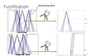
Low Medium High
Workload
1
0
α β γ δ
Bad OK Good
Response Time
1
0
λ μ ν
of w and rt that correspond to the state of the system, s(t) (cf.
Step 4 in Algorithm 1). The control signal sa represents the
action a that the controller take at each loop. We define the
reward signal r(t) based on three criteria: (i) numbers of the
desired response time violations, (ii) the amount of resource
acquired, and (iii) throughput, as follows:
r(t) = U(t) U(t 1), (6)
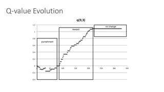
where U(t) is the utility value of the system at time t. Hence,
if a controlling action leads to an increased utility, it means
that the action is appropriate. Otherwise, if the reward is close
to zero, it implies that the action is not effective. A negative
reward (punishment) warns that the situation becomes worse
after taking the action. The utility function is defined as:
U(t) = w1 ·
th(t)
thmax
+w2 ·(1
vm(t)
vmmax
)+w3 ·(1 H(t)) (7)
H(t) =
8
><
>:
(rt(t) rtdes)
rtdes
rtdes rt(t) 2 · rtdes
1 rt(t) 2 · rtdes
0 rt(t) rtdes
where th(t), vm(t) and rt(t) are throughput, number of worker
roles and response time of the system, respectively. w1,w2 and
w3 are their corresponding weights determining their relative
o possible but due to the intricacies of updating
e, we consider this as a natural future extension
r the problem areas that requires coordination
controllers, see [9].
ion. The controller receives the current values
t correspond to the state of the system, s(t) (cf.
rithm 1). The control signal sa represents the
e controller take at each loop. We define the
(t) based on three criteria: (i) numbers of the
e time violations, (ii) the amount of resource
ii) throughput, as follows:
r(t) = U(t) U(t 1), (6)
he utility value of the system at time t. Hence,
action leads to an increased utility, it means
s appropriate. Otherwise, if the reward is close
ies that the action is not effective. A negative
ment) warns that the situation becomes worse
action. The utility function is defined as:
h(t)
max
+w2 ·(1
vm(t)
vmmax
)+w3 ·(1 H(t)) (7)
Code:
https://github.com/pooyanjamshidi/Fuzzy-Q-Learning](https://image.slidesharecdn.com/self-learningcloudcontrollers-sharif6-160414051512/85/Fuzzy-Self-Learning-Controllers-for-Elasticity-Management-in-Dynamic-Cloud-Architectures-35-320.jpg)

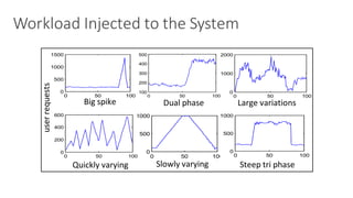


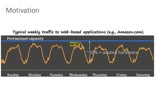
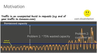
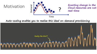
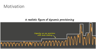
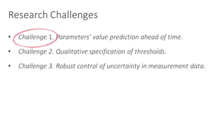
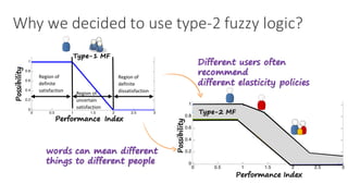
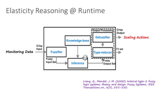
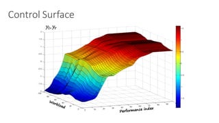
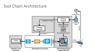
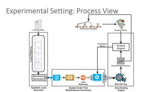
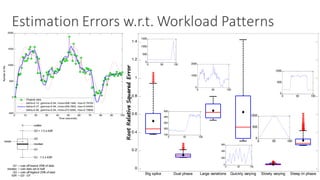
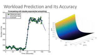
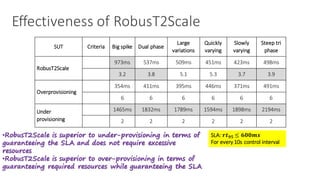
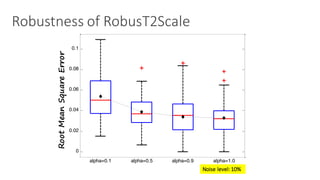
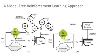
(1) The document discusses challenges in managing elasticity in cloud architectures due to unpredictable demand and uncertainty in measurements. (2) It proposes a fuzzy self-learning controller called RobusT2Scale that uses type-2 fuzzy logic to qualitatively specify thresholds and make robust scaling decisions despite uncertainty. (3) Experimental results show that RobusT2Scale is able to guarantee service level agreements while avoiding over- and under-provisioning of resources compared to other approaches.


![[241]large scale search with polysemous codes](https://cdn.slidesharecdn.com/ss_thumbnails/241large-scalesearchwithpolysemouscodes-171017003327-thumbnail.jpg?width=640&height=640&fit=bounds)


