Download to read offline
![The Flow Equation (cont.)
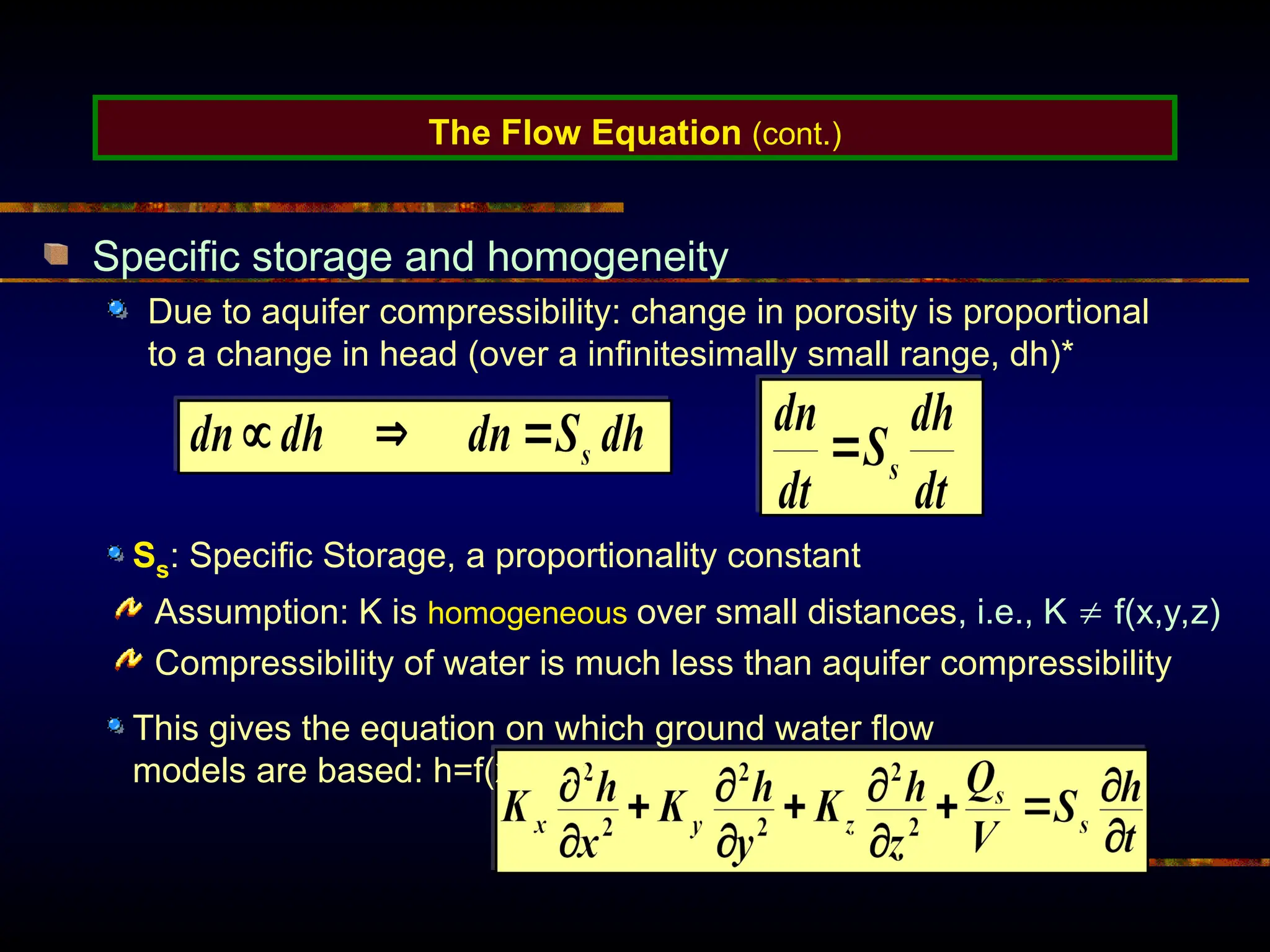
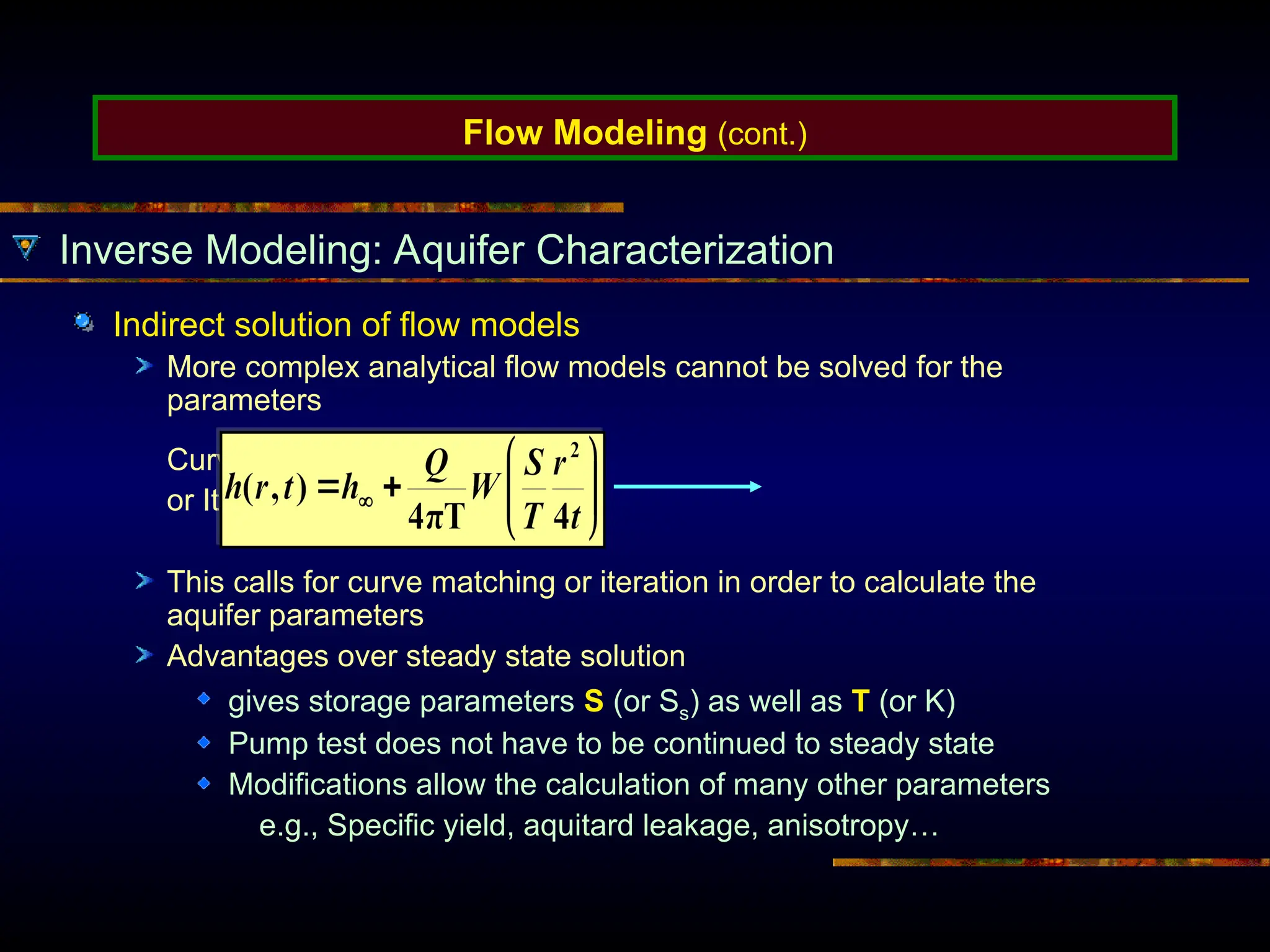
Flow Equation Simplifications
0
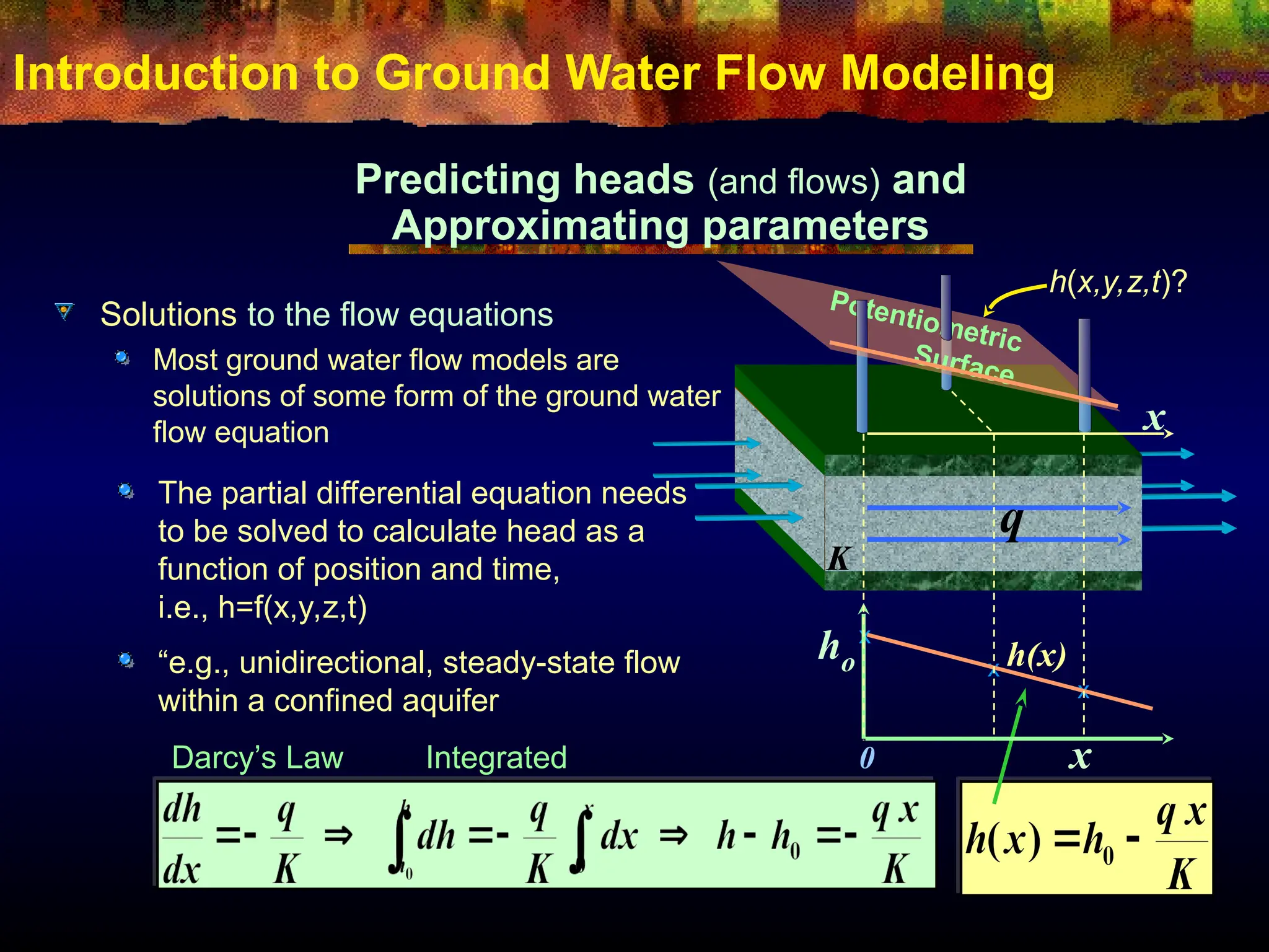
Our job is not yet finished, h=f(x,y,z,t)?
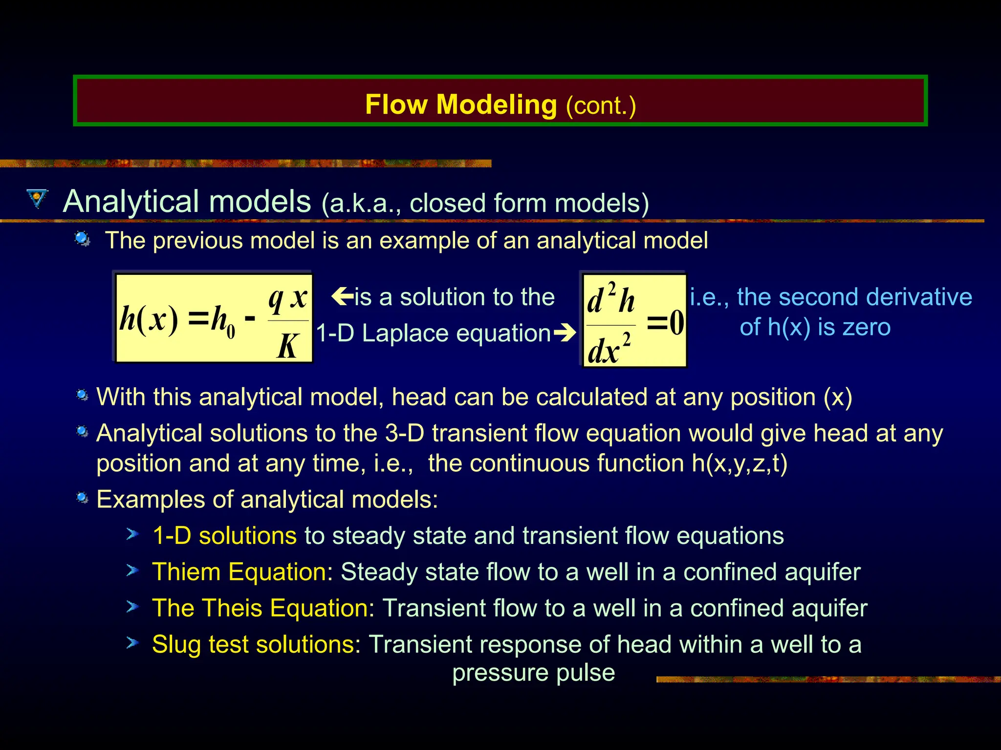
Isotropic, 2-D, steady state flow equation
(without source term), a.k.a.: The Laplace Equation
2-D, horizontally isotropic flow equation
Kx=Ky=Kh
T=Kh b units: [L2
/T], S=Ss b
Ah: horizontal area of recharge
Ss/Kh=S/T hydraulic diffusivity
Two dimensional flow equation
Horizontal flow (Dupuit assumption)
Thus: dh/dz = 0
Steady State Flow Equation
If inflow = out flow, Net inflow = 0
Change in storage = 0
0
0 0](https://image.slidesharecdn.com/finitedifferencegwmodeling-compatibilitymode-repaired-241025144050-b05461d0/75/FiniteDifference-GW-modeling-Compatibility-Mode-Repaired-ppt-10-2048.jpg)


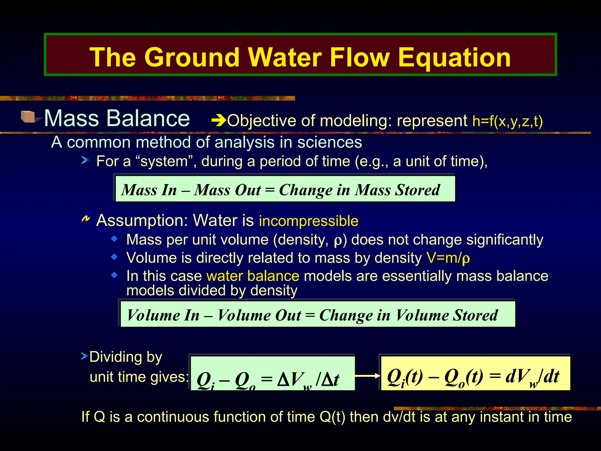
The document provides an introduction to ground water flow modeling, emphasizing the importance of the mass balance equation and the flow equation in modeling strategies. It discusses analytical and numerical methods for solving flow equations, including forward and inverse modeling, as well as the use of finite difference methods for approximating solutions. The limitations of analytical models and the need for more complex numerical modeling to address geological complexities are also highlighted.


![1 Lesson1[1] GW hydrology.ppt](https://cdn.slidesharecdn.com/ss_thumbnails/1lesson11gwhydrology-230731023014-744827f1-thumbnail.jpg?width=640&height=640&fit=bounds)


