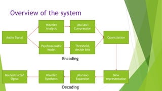
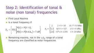
This document describes an audio compression system using discrete wavelet transform and a psychoacoustic model. The system analyzes audio signals using wavelet decomposition, applies a psychoacoustic model to estimate masking thresholds, quantizes coefficients below the thresholds, and encodes the results. Evaluation showed the system achieved over 50% bit rate reduction with transparent quality on music signals like violin, drums, piano and vocals based on subjective listening tests.

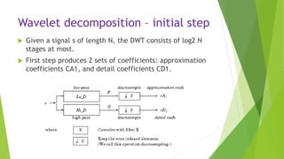
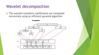
![Recursive wavelet decomposition
The wavelet decomposition of the signal s analyzed at
level j has the following structure: [cAj, cDj, ..., cD1].](https://image.slidesharecdn.com/finalpresentation-170328191808/85/Final-presentation-24-320.jpg)
![References
[1] D. Sinha and A. Tewfik. “Low Bit Rate Transparent Audio Compression using
Adapted Wavelets”, IEEE Trans. ASSP, Vol. 41, No. 12, December 1993
[2] T. Painter and A. Spanias, “A review of algorithms for perceptual coding of
digital audio signals,” DSP-97, 1977.
[3] I. Daubechies, “Orthonormal bases of compactly supported wavelets”,
Commun. Pure Appl. Math.. vol 41, pp 909-996, Nov 1988
[4] ISO/IEC JTC1/SC29/WG11 MPEG, IS11172-3 “Information Technology - Coding of
Moving Pictures and Associated Audio for Digital Storage Media at up to About 1.5
Mbit/s, Part 3: Audio” 1992. (“MPEG-1”)
[5] R. Hellman, “Asymmetry of Masking Between Noise and Tone,” Percep. and
Psychphys., pp. 241-246, vol.11, 1972
[6] M. Schroeder, et al., “Optimizing Digital Speech Coders by Exploiting Masking
Properties of the Human Ear,” J. Acoust. Soc. Am., pp. 1647-1652, Dec. 1979
[7] E. Zwicker and H. Fastl, Psychoacoustics Facts and Models, Springer-Verlag,
1990
[8] C. Burrus, R. A. Gopinath and H. Guo, “Introduction to Wavelets & Wavelet
Transforms”, Prentice-Hall 1998](https://image.slidesharecdn.com/finalpresentation-170328191808/85/Final-presentation-34-320.jpg)