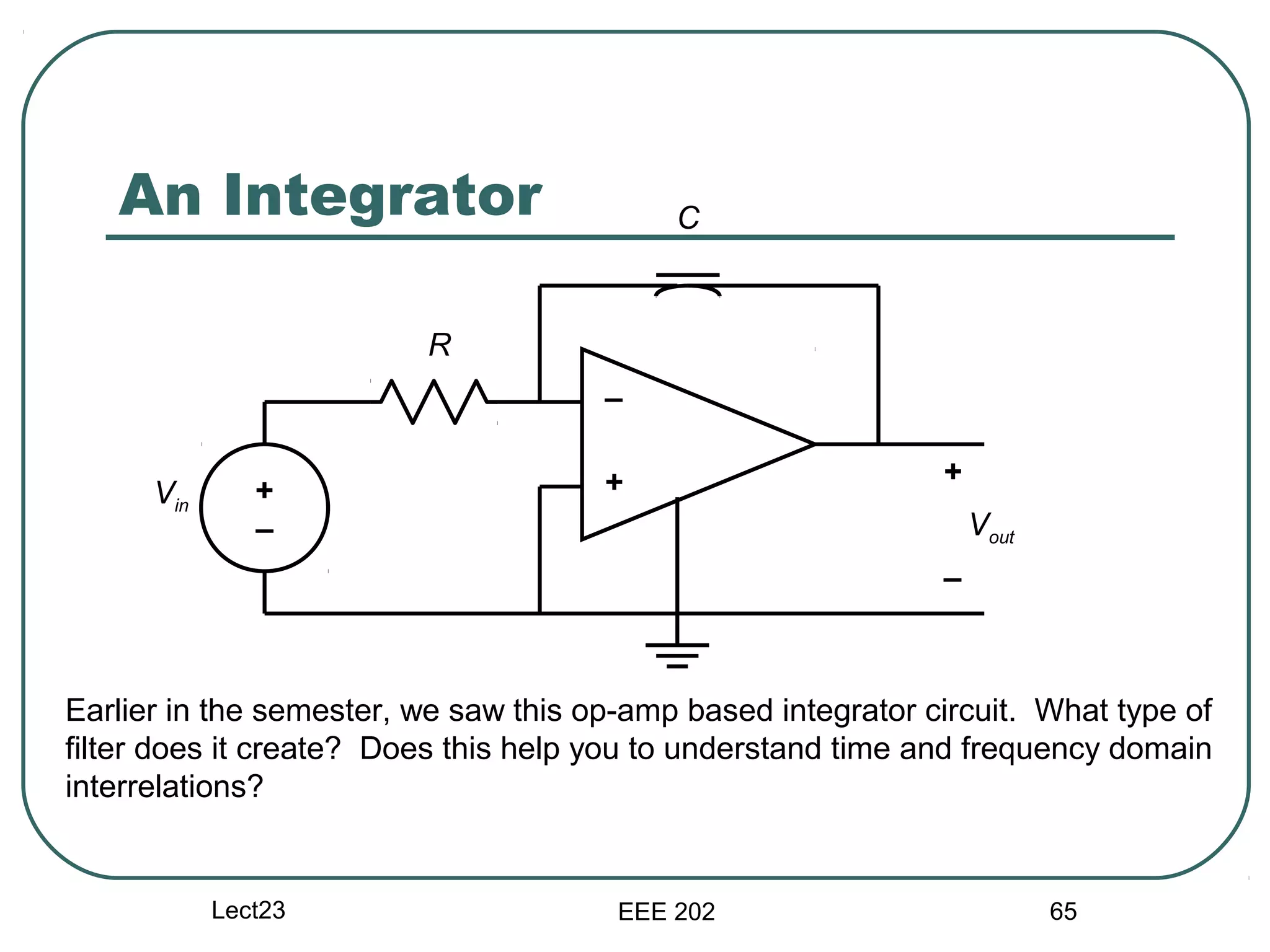
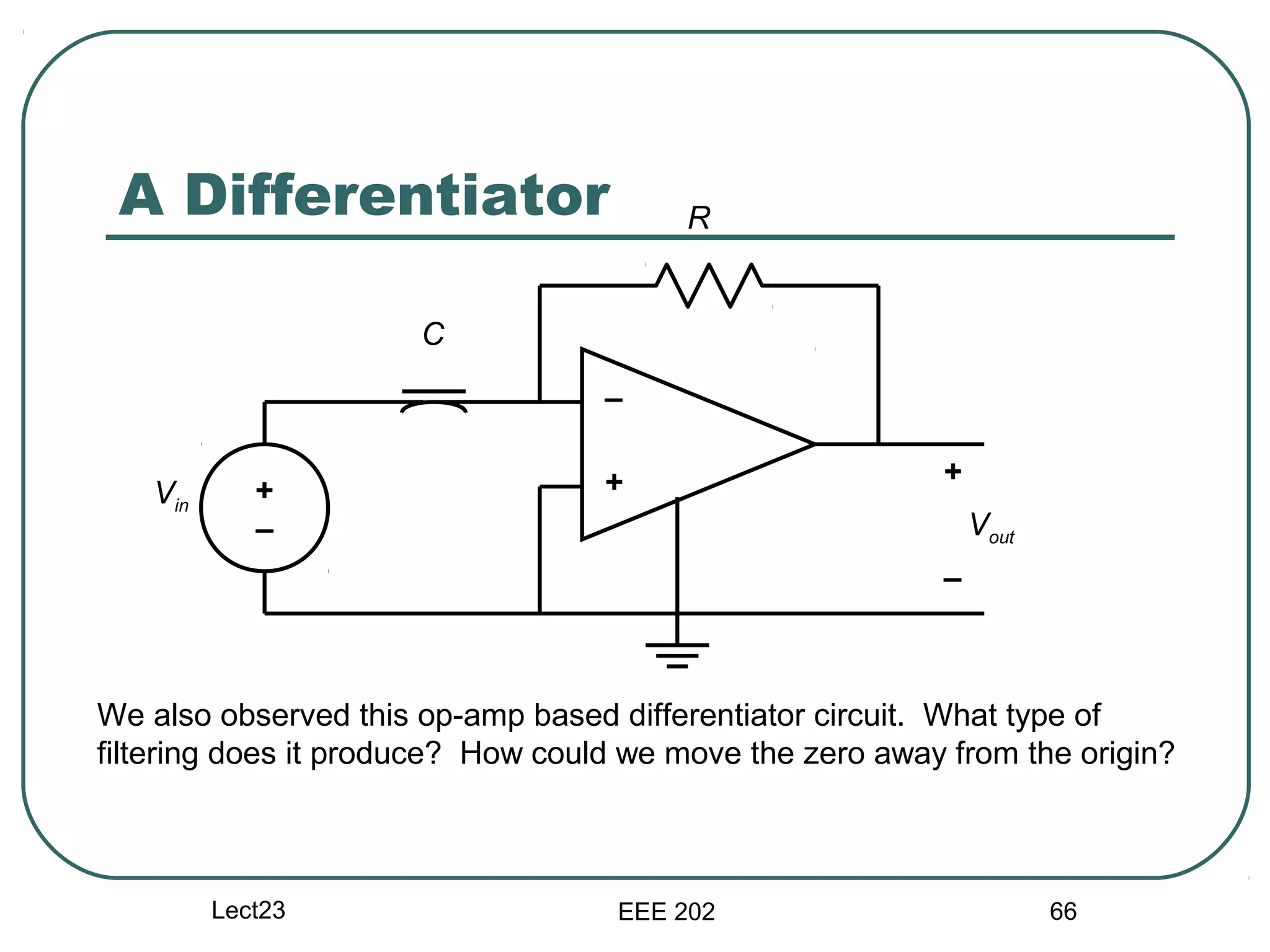
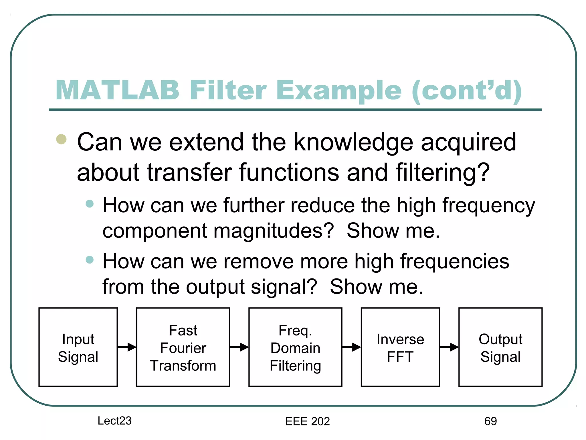
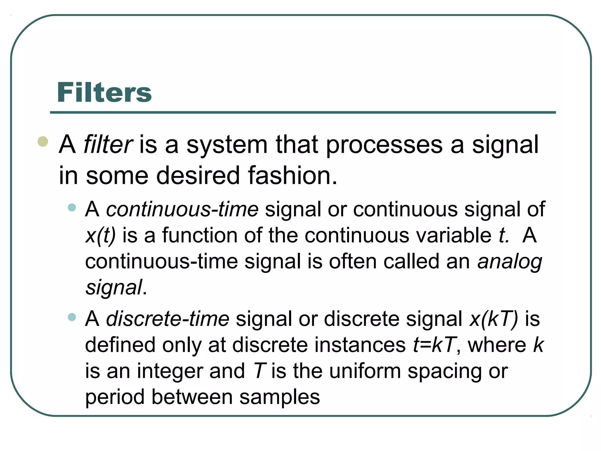
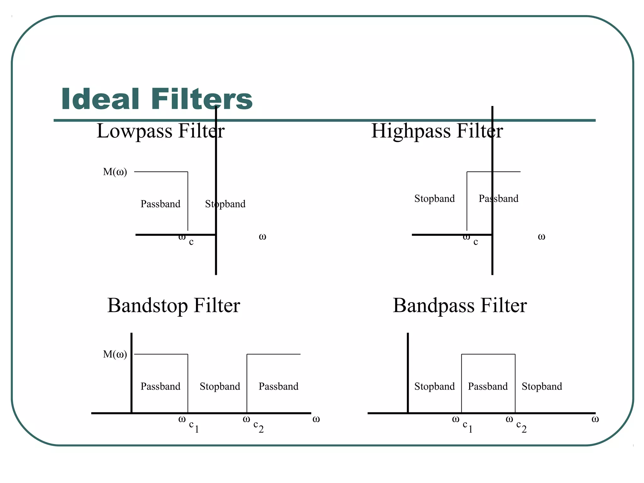
The document discusses different types of filters and their frequency responses. It describes that filters can be either analog and process continuous signals, or digital and process discrete signals. There are four main types of filters: lowpass, highpass, bandstop, and bandpass. The frequency response of these filters can be modeled using concepts like poles, zeros, break/corner frequencies, and Bode plots. Bode plots use logarithmic scales to show how the magnitude and phase of a filter's transfer function change over frequency.

1. Active Filters

2. Filters
A filter is a system that processes a signal
in some desired fashion.
• A continuous-time signal or continuous signal of
x(t) is a function of the continuous variable t. A
continuous-time signal is often called an analog
signal.
• A discrete-time signal or discrete signal x(kT) is
defined only at discrete instances t=kT, where k
is an integer and T is the uniform spacing or
period between samples

3. Types of Filters
 There are two broad categories of filters:
• An analog filter processes continuous-time signals
• A digital filter processes discrete-time signals.
 The analog or digital filters can be subdivided
into four categories:
• Lowpass Filters
• Highpass Filters
• Bandstop Filters
• Bandpass Filters

4. Analog Filter Responses
H(f) H(f)
0 f 0 f
fc fc
Ideal “brick wall” filter Practical filter

5. Ideal Filters
Lowpass Filter Highpass Filter
M(ω)
Stopband Passband
Passband Stopband
ωc ω ωc ω
Bandstop Filter Bandpass Filter
M(ω)
Passband Stopband Passband Stopband Passband Stopband
ωc ωc ω ωc ωc ω
1 2 1 2

6.  There are a number of ways to build
filters and of these passive and active
filters are the most commonly used in
voice and data communications.

7. Passive filters
 Passive filters use resistors, capacitors, and
inductors (RLC networks).
 To minimize distortion in the filter
characteristic, it is desirable to use inductors
with high quality factors (remember the model
of a practical inductor includes a series
resistance), however these are difficult to
implement at frequencies below 1 kHz.
• They are particularly non-ideal (lossy)
• They are bulky and expensive

8.  Active
filters overcome these drawbacks
and are realized using resistors,
capacitors, and active devices (usually
op-amps) which can all be integrated:
• Active filters replace inductors using op-amp
based equivalent circuits.

9. Op Amp Advantages
 Advantages of active RC filters include:
• reduced size and weight, and therefore parasitics
• increased reliability and improved performance
• simpler design than for passive filters and can realize
a wider range of functions as well as providing voltage
gain
• in large quantities, the cost of an IC is less than its
passive counterpart

10. Op Amp Disadvantages
 Active RC filters also have some disadvantages:
• limited bandwidth of active devices limits the highest
attainable pole frequency and therefore applications above
100 kHz (passive RLCfilters can be used up to 500 MHz)
• the achievable quality factor is also limited
• require power supplies (unlike passive filters)
• increased sensitivity to variations in circuit parameters
caused by environmental changes compared to passive
filters
 For many applications, particularly in voice and data
communications, the economic and performance
advantages of active RC filters far outweigh their
disadvantages.

11. Bode Plots
 Bode plots are important when
considering the frequency response
characteristics of amplifiers. They plot
the magnitude or phase of a transfer
function in dB versus frequency.

12. The decibel (dB)
Two levels of power can be compared using a
unit of measure called the bel.
P2
B = log10
P1
The decibel is defined as:
1 bel = 10 decibels (dB)

13. P2
dB = 10 log10
P1
A common dB term is the half power point
which is the dB value when the P2 is one-
half P1.
1
10 log10 = −3.01 dB ≈ −3 dB
2

14. Logarithms
A logarithm is a linear transformation used
to simplify mathematical and graphical
operations.
 A logarithm is a one-to-one correspondence.

15. Any number (N) can be represented as a
base number (b) raised to a power (x).
N = (b) x
The value power (x) can be determined by
taking the logarithm of the number (N) to
base (b).
x = log b N

16.  Although there is no limitation on the
numerical value of the base, calculators are
designed to handle either base 10 (the
common logarithm) or base e (the natural
logarithm).
 Any base can be found in terms of the
common logarithm by:
1
log q w = log10 w
log10 q

17. Properties of Logarithms
 The common or natural  The log of the quotient
logarithm of the number of two numbers is the
1 is 0. log of the numerator
 The log of any number minus the
less than 1 is a negative denominator.
number.  The log a number
 The log of the product of taken to a power is
two numbers is the sum equal to the product of
of the logs of the the power and the log
numbers. of the number.

18. Poles & Zeros of the transfer
function
 pole—value of s where the denominator
goes to zero.
 zero—value of s where the numerator
goes to zero.

19. Single-Pole Passive Filter
R vout ZC 1 / sC
= =
vin R + Z C R + 1 / sC
vin C vout 1 1 / RC
= =
sCR + 1 s + 1 / RC
 Firstorder low pass filter
 Cut-off frequency = 1/RC rad/s
 Problem : Any load (or source)
impedance will change frequency
response.

20. Single-Pole Active Filter
R
vin C
vout
 Same frequency response as passive
filter.
 Buffer amplifier does not load RC
network.
 Output impedance is now zero.

21. Low-Pass and High-Pass
Designs
High Pass Low Pass
vout 1 1
= =
vin 1 1 + sRC vout 1 / RC
+1
sCR sCR =
sRC s vin s + 1 / RC
= =
RC ( s + 1 / RC ) ( s + 1 / RC )

22. To understand Bode plots, you need to
use Laplace transforms! R
The transfer function
of the circuit is: V in (s)
Vo ( s ) 1 / sC 1
Av = = =
Vin ( s ) R + 1 / sC sRC + 1

23. Break Frequencies
Replace s with jω in the transfer function:
1 1 1
Av ( f ) = = =
jωRC + 1 1 + j 2πRCf  f 
1 + j 
f 
 b
where fc is called the break frequency, or corner
frequency, and is given by:
1
fc =
2πRC

24. Corner Frequency
 The significance of the break frequency is that
it represents the frequency where
Av(f) = 0.707∠-45°.
 This is where the output of the transfer function
has an amplitude 3-dB below the input
amplitude, and the output phase is shifted by
-45° relative to the input.
 Therefore, fc is also known as the 3-dB
frequency or the corner frequency.

26. Bode plots use a logarithmic scale for
frequency.
One decade
10 20 30 40 50 60 70 80 90 100 200
where a decade is defined as a range of
frequencies where the highest and lowest
frequencies differ by a factor of 10.

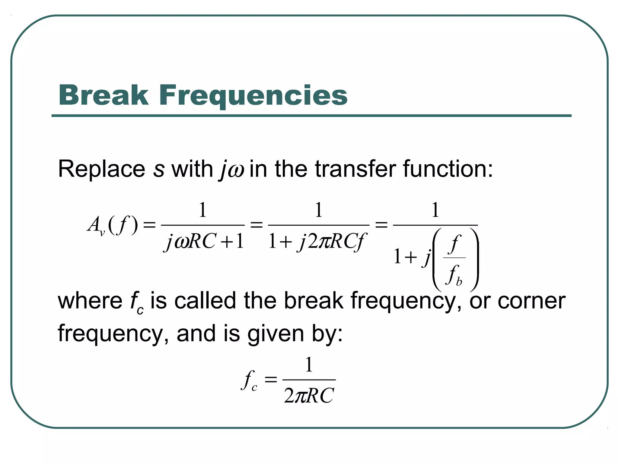
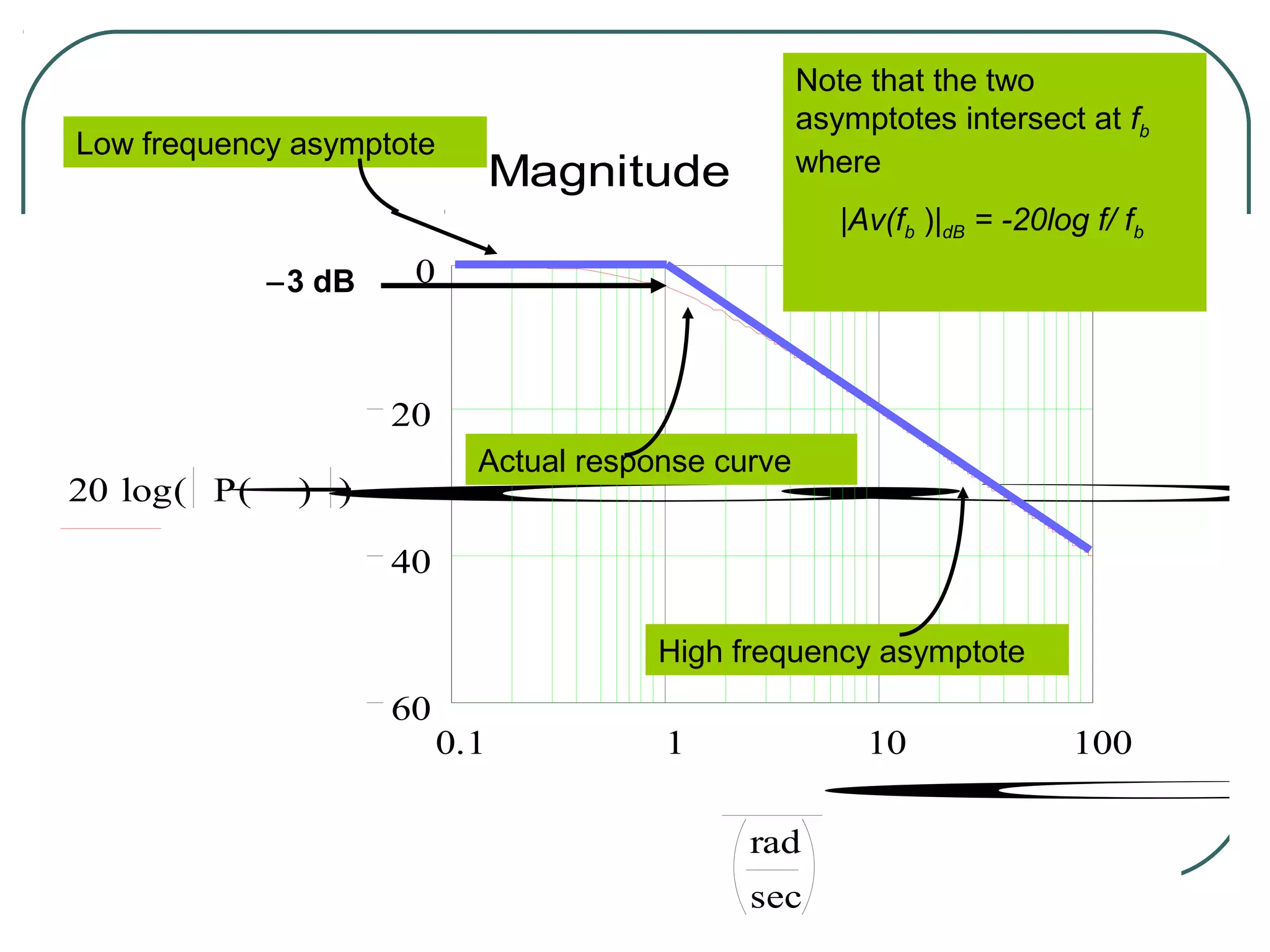
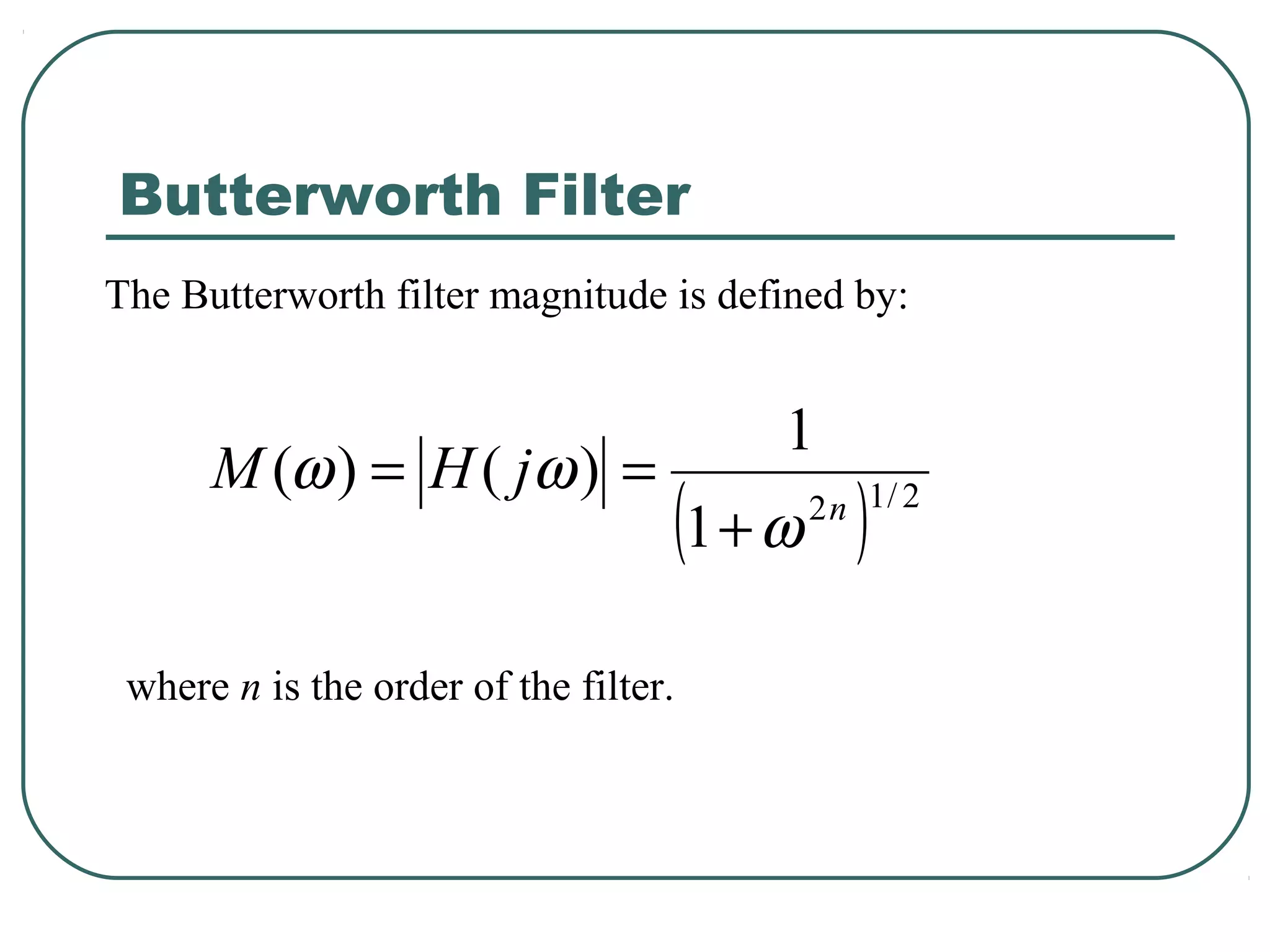
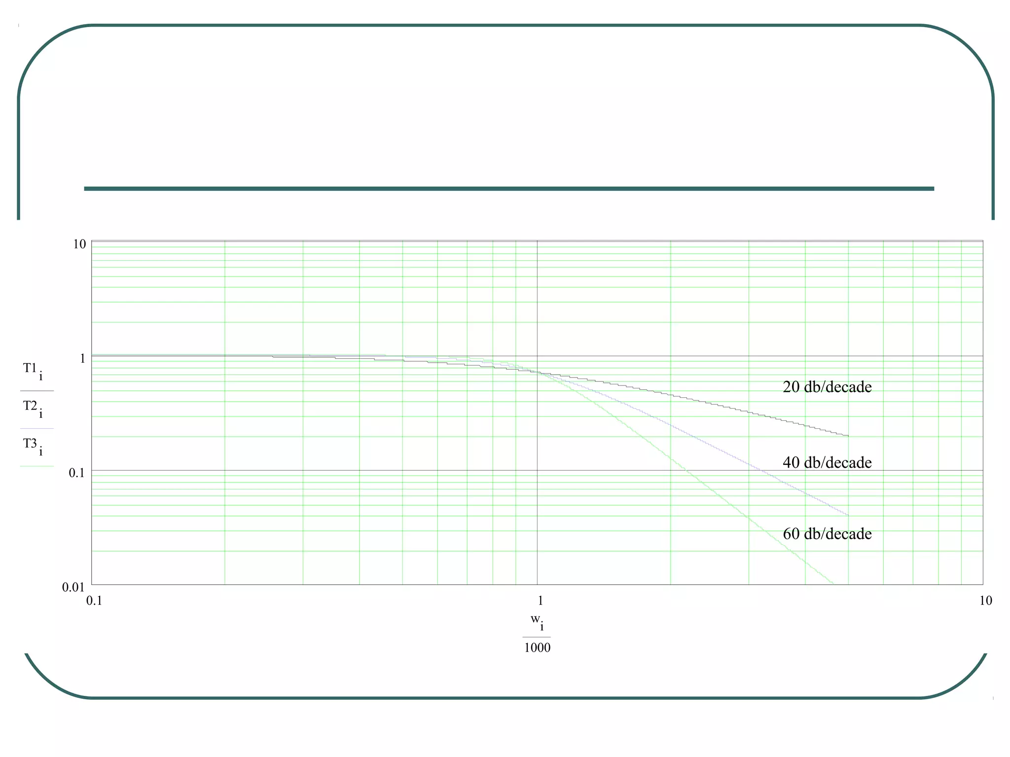
27.  Consider the magnitude of the transfer
function: 1
Av ( f ) =
1 + ( f / fb )
2
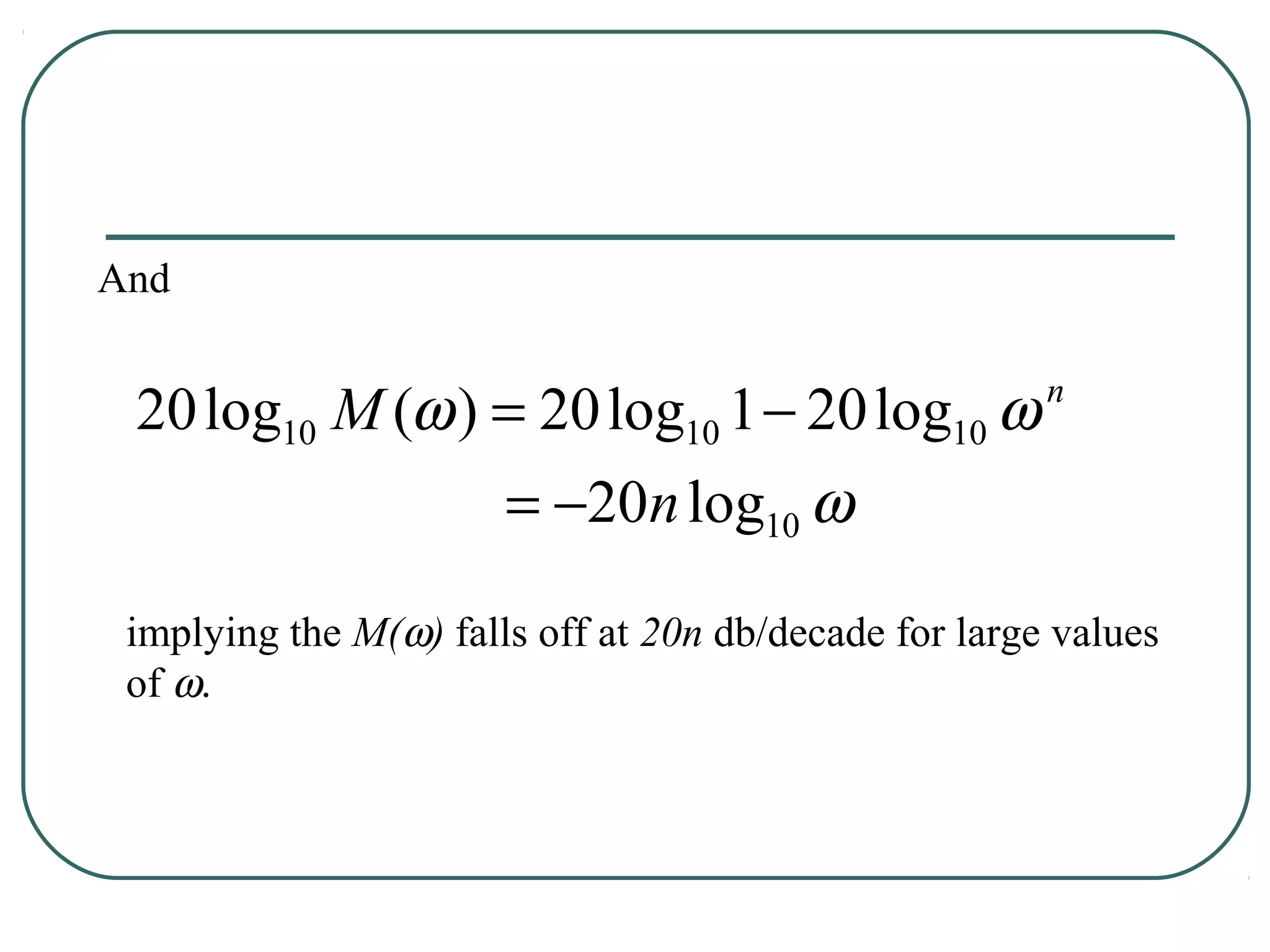
Expressed in dB, the expression is
Av ( f ) dB = 20 log 1 − 20 log 1 + ( f / f b )
2
[
= −20 log 1 + ( f / f b ) = −10 log 1 + ( f / f b )
2 2
]
= −20 log( f / f b )

28.  Lookhow the previous expression
changes with frequency:
• at low frequencies f<< f , |Av|
b dB = 0 dB
• low frequency asymptote
• at high frequencies f>>f , b
|Av(f)|dB = -20log f/ fb
• high frequency asymptote

29. Note that the two
asymptotes intersect at fb
Low frequency asymptote
Magnitude where
|Av(fb )|dB = -20log f/ fb
−3 dB 0
20
Actual response curve
20 .
log ( P ( ω
) )
40
High frequency asymptote
60
0.1 1 10 100
ω
rad
sec

30.  The technique for approximating a filter
function based on Bode plots is useful
for low order, simple filter designs
 More complex filter characteristics are
more easily approximated by using some
well-described rational functions, the
roots of which have already been
tabulated and are well-known.

31. Real Filters
 The approximations to the ideal filter are
the:
• Butterworth filter
• Chebyshev filter
• Cauer (Elliptic) filter
• Bessel filter

32. Standard Transfer Functions
 Butterworth
• Flat Pass-band.
• 20n dB per decade roll-off.
 Chebyshev
• Pass-band ripple.
• Sharper cut-off than Butterworth.
 Elliptic
• Pass-band and stop-band ripple.
• Even sharper cut-off.
 Bessel
• Linear phase response – i.e. no signal distortion in
pass-band.

34. Butterworth Filter
The Butterworth filter magnitude is defined by:
1
M (ω ) = H ( jω ) =
(1 + ω )
2 n 1/ 2
where n is the order of the filter.

35. From the previous slide:
M (0) = 1
1
M (1) = for all values of n
2
For large ω:
1
M (ω ) ≅ n
ω

36. And
20 log10 M (ω ) = 20 log10 1 − 20 log10 ω n
= −20n log10 ω
implying the M(ω) falls off at 20n db/decade for large values
of ω.

37. 10
1
T1
i
20 db/decade
T2
i
T3
i
40 db/decade
0.1
60 db/decade
0.01
0.1 1 10
w
i
1000

38. To obtain the transfer function H(s) from the magnitude
response, note that
2 1
M (ω ) = H ( jω ) = H ( jω ) H (− jω ) =
2
1+ ω ( ) 2 n

39. Because s = jω for the frequency response, we have s2 = − ω2.
1 1
H ( s) H (− s) = =
(
1+ − s )
2 n
1 + ( − 1) s
n 2n
The poles of this function are given by the roots of
1 + ( − 1) s − j ( 2 k −1)π
n 2n
= −1 = e , k = 1,2,  ,2n

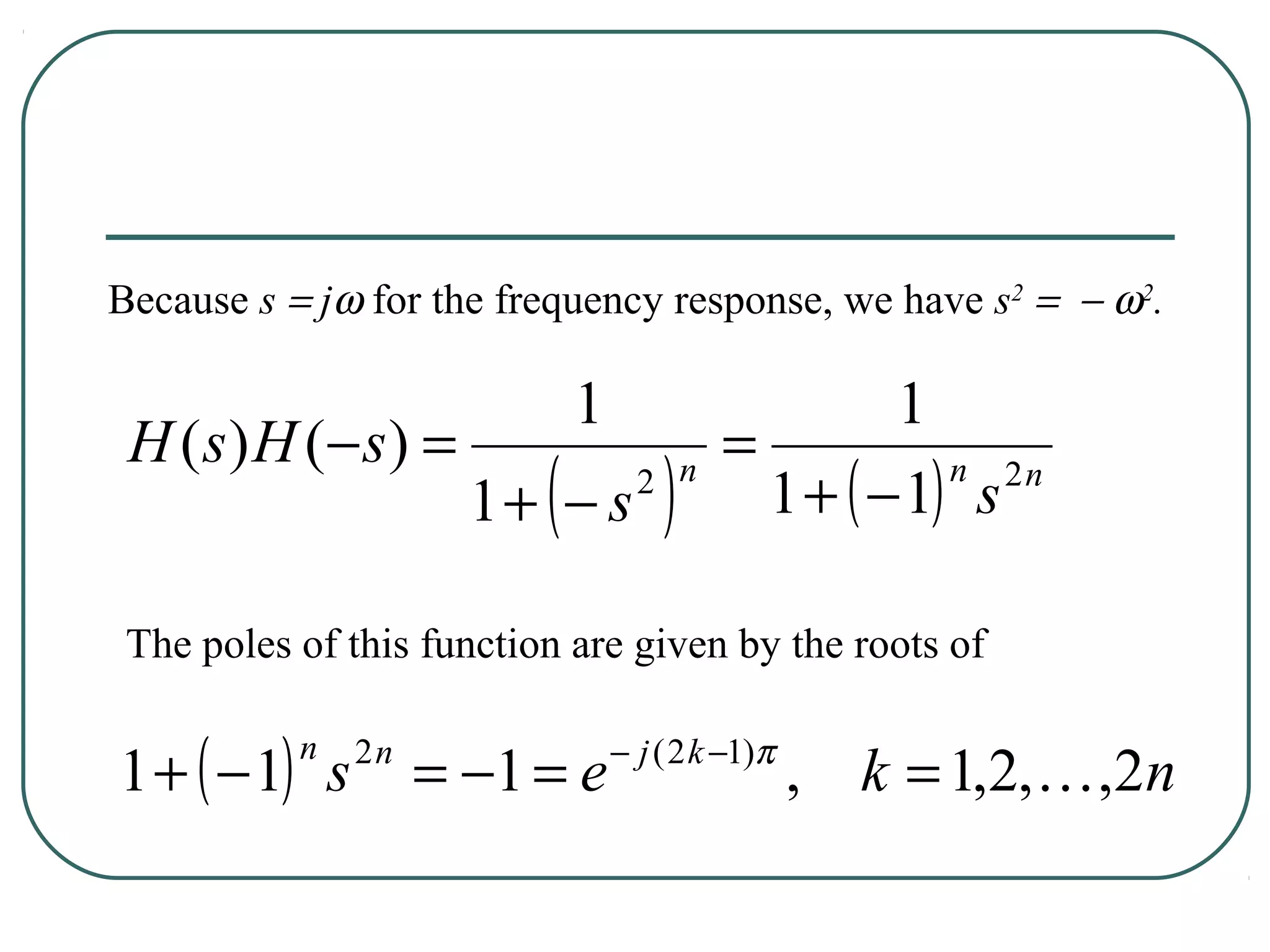
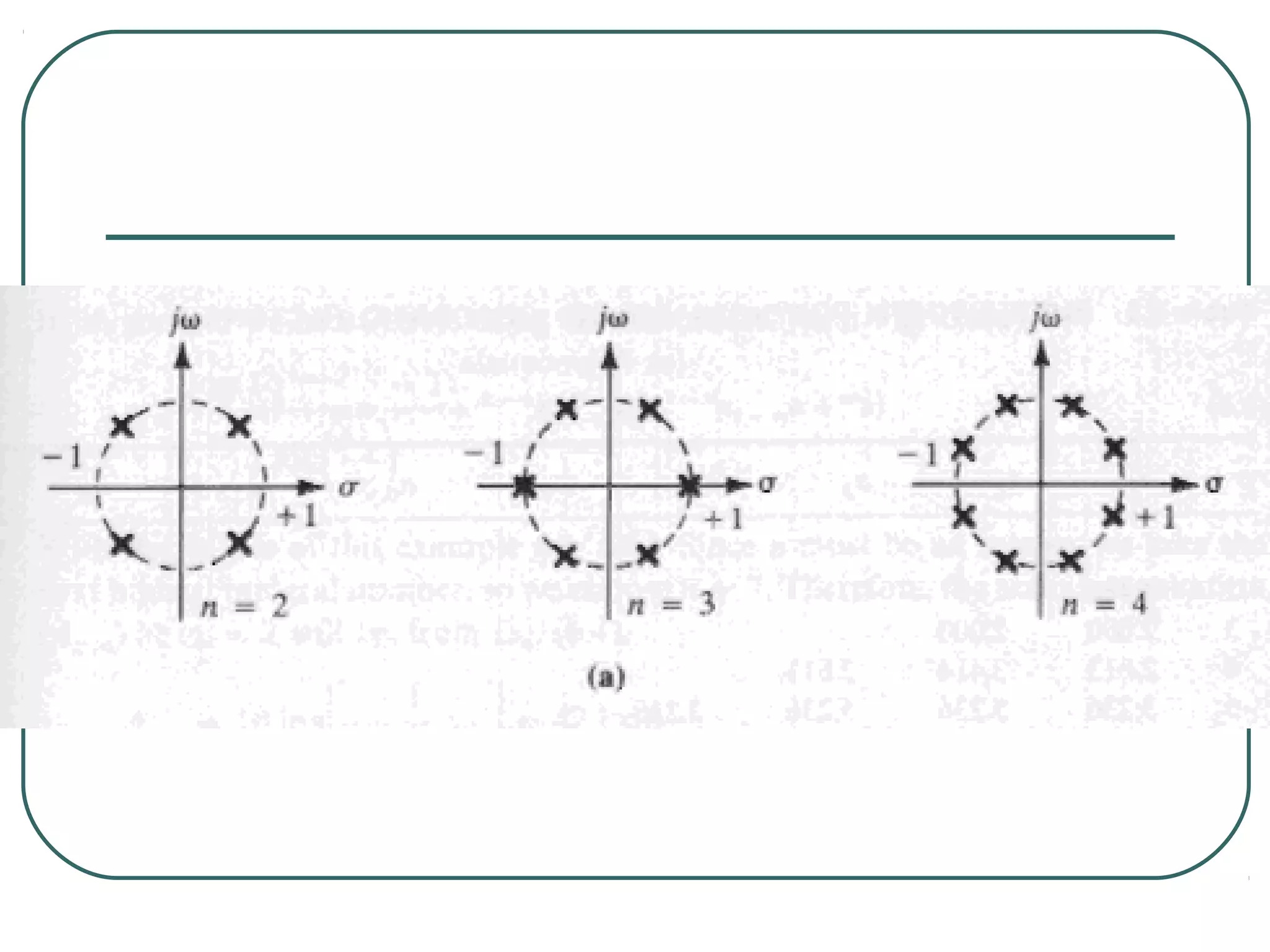
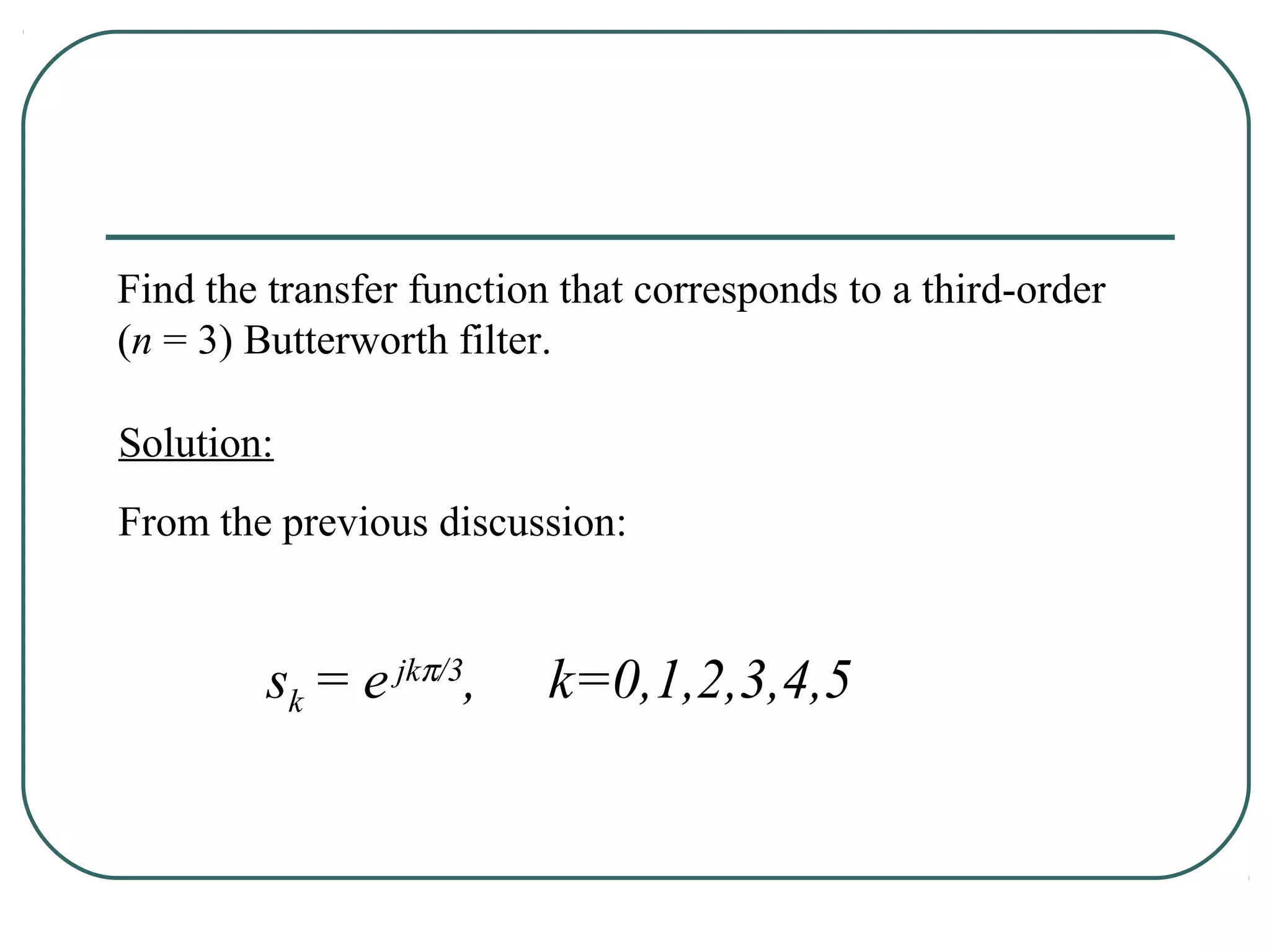
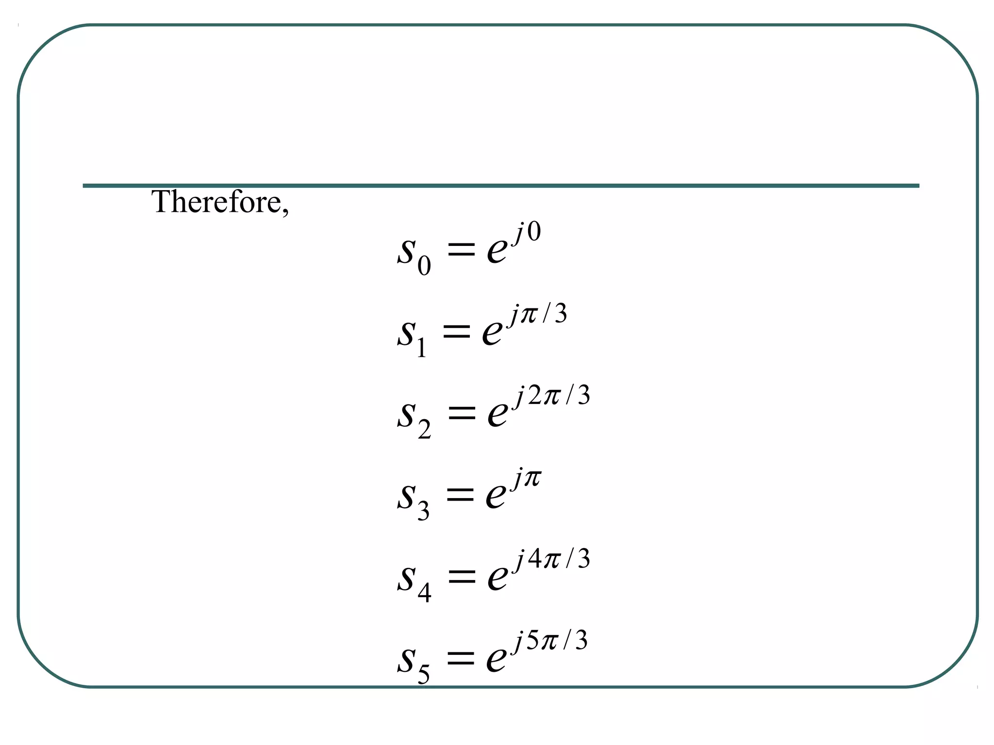
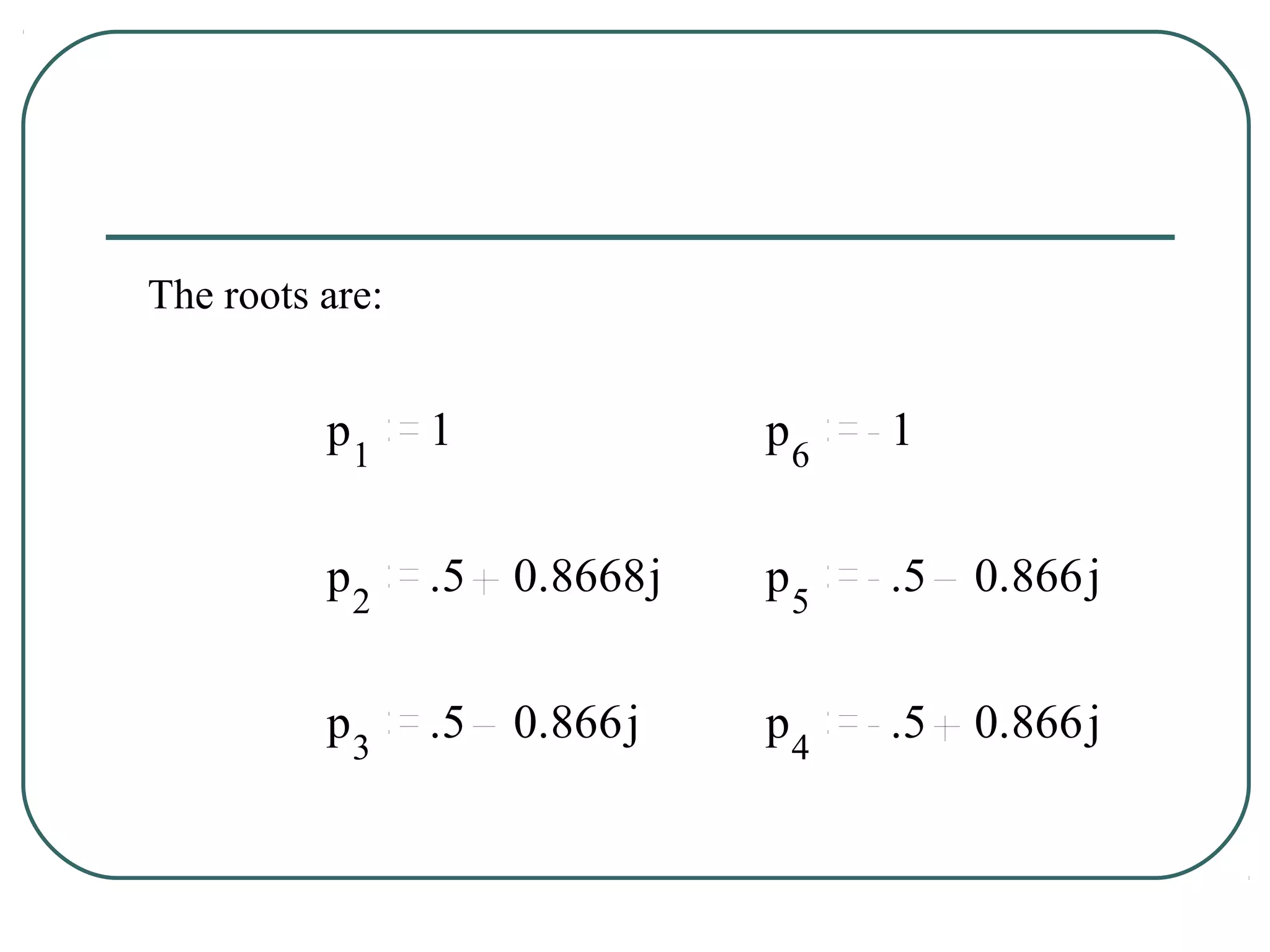
40. The 2n pole are:
e j[(2k-1)/2n]π n even, k = 1,2,...,2n
sk =
e j(k/n)π n odd, k = 0,1,2,...,2n-1
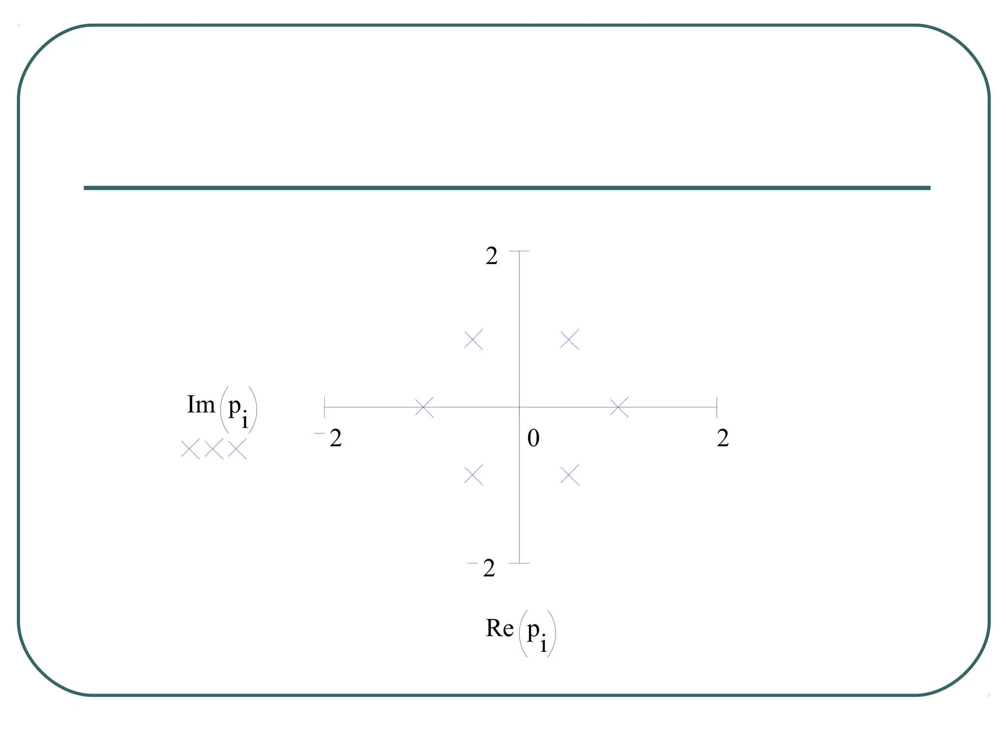
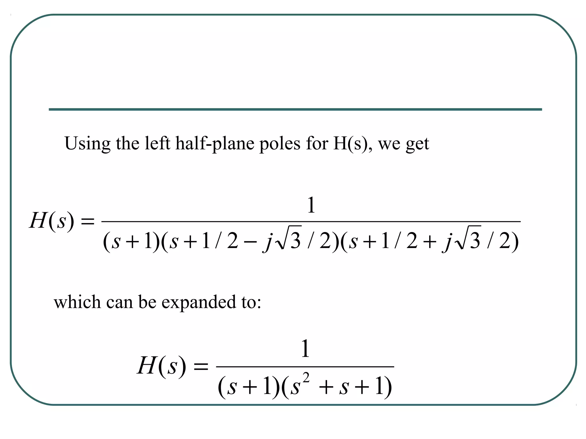
Note that for any n, the poles of the normalized Butterworth
filter lie on the unit circle in the s-plane. The left half-plane
poles are identified with H(s). The poles associated with
H(-s) are mirror images.

43. Recall from complex numbers that the rectangular form
of a complex can be represented as:
z = x + jy
Recalling that the previous equation is a phasor, we can
represent the previous equation in polar form:
z = r ( cosθ + j sin θ )
where
x = r cosθ and y = r sin θ

44. Definition: If z = x + jy, we define e z = e x+ jy to be the
complex number
e = e (cos y + j sin y )
z x
Note: When z = 0 + jy, we have
e jy = (cos y + j sin y )
which we can represent by symbol:
jθ
e

45. The following equation is known as Euler’s law.
jθ
e = (cosθ + j sin θ )
Note that
cos( − θ ) = cos( − θ ) even function
sin ( − θ ) = − sin (θ ) odd function

46. This implies that
− jθ
e = (cosθ − j sin θ )
This leads to two axioms:
jθ − jθ
e +e jθ − jθ
e −e
cos θ = and sin θ =
2 2j

47.  Observe that e jθ represents a unit vector
which makes an angle θ with the
positivie x axis.

48. Find the transfer function that corresponds to a third-order
(n = 3) Butterworth filter.
Solution:
From the previous discussion:
sk = e jkπ/3, k=0,1,2,3,4,5

49. Therefore,
s0 = e j0
jπ / 3
s1 = e
j 2π / 3
s2 = e
jπ
s3 = e
j 4π / 3
s4 = e
j 5π / 3
s5 = e

50. The roots are:
p1 1 p6 1
p2 .5 ..
0.8668j p5 .5 0.866 j
p3 .5 . .
0.866j p4 .5 0.866 j

51. 2
Im p
i
2 0 2
2
Re p
i

52. Using the left half-plane poles for H(s), we get
1
H ( s) =
( s + 1)( s + 1 / 2 − j 3 / 2)( s + 1 / 2 + j 3 / 2)
which can be expanded to:
1
H ( s) =
( s + 1)( s + s + 1)
2

53.  The factored form of the normalized
Butterworth polynomials for various order
n are tabulated in filter design tables.

54. n Denominator of H(s) for Butterworth Filter
1 s+1
2 s2 + 1.414s + 1
3 (s2 + s + 1)(s + 1)
4 (s2 + 0.765 + 1)(s2 + 1.848s + 1)
5 (s + 1) (s2 + 0.618s + 1)(s2 + 1.618s + 1)
6 (s2 + 0.517s + 1)(s2 + 1.414s + 1 )(s2 + 1.932s + 1)
7 (s + 1)(s2 + 0.445s + 1)(s2 + 1.247s + 1 )(s2 + 1.802s + 1)
8 (s2 + 0.390s + 1)(s2 + 1.111s + 1 )(s2 + 1.663s + 1 )(s2 + 1.962s + 1)

55. Frequency Transformations

56. So far we have looked at the Butterworth filter
with a normalized cutoff frequency
ω c = 1 rad / sec
By means of a frequency transformation, we
can obtain a lowpass, bandpass, bandstop, or
highpass filter with specific cutoff frequencies.

57. Lowpass with Cutoff Frequency
ωu
 Transformation:
sn = s / ω u

58. Highpass with Cutoff Frequency
ωl
 Transformation:
sn = ω l / s

59. Bandpass with Cutoff
Frequencies ωl and ωu
 Transformation:
F
G
s2 + ω 2 ω 0 s ω 0 I
J
sn = =
H +
K
0
Bs B ω0 s
where
ω 0 = ω uω l
B = ωu −ωl

60. Bandstop with Cutoff
Frequencies ωl and ωu
 Transformation:
Bs B
sn = 2
s +ω0 2
=
Fs + ω I
ω G J
H sK
0
ω
0
0

61. Active Filters
 To achieve a gain > 1, we need to utilize
an op-amp based circuit to form an
active filter
 We can design all the common filter
types using op-amp based active filters
 Recall for an ideal op-amp that
V+ = V– I+ = I – = 0
Lect23 EEE 202 61

62. Op Amp Model
Non-inverting V+
input
+
Rout Vo
Rin
+
– –
Inverting
input A(V+ –V– )
V–
Lect23 EEE 202 62

63. Non-inverting Op-Amp Circuit
+ Vout
H ( jω ) =
– + Vin
Z2
Vin + = 1+
– Z2 Vout Z1
Z1
–
Lect23 EEE 202 63

64. Inverting Op-Amp Circuit
Z2
Z1 –
–
Vin + +
– Vout
+
Vout Z 2
H ( jω ) = =
Vin Z1
Lect23 EEE 202 64

65. An Integrator C
R
–
+ +
Vin +
– Vout
–
Earlier in the semester, we saw this op-amp based integrator circuit. What type of
filter does it create? Does this help you to understand time and frequency domain
interrelations?
Lect23 EEE 202 65

66. A Differentiator R
C
–
+ +
Vin +
– Vout
–
We also observed this op-amp based differentiator circuit. What type of
filtering does it produce? How could we move the zero away from the origin?
Lect23 EEE 202 66

67. Practical Example
 Youare shopping for a stereo system,
and the following specifications are
quoted:
• Frequency range: –6 dB at 65 Hz and 22 kHz
• Frequency response: 75 Hz to 20 kHz ±3 dB
 What do these specs really mean?
• Note that the human hearing range is around
20 Hz to 20 kHz (audible frequencies)
 Could
you draw a rough Bode
(magnitude) plot for the stereo system?
Lect23 EEE 202 67

68. MATLAB Filter Example
 How can we filter a real measurement
signal?
 One method involves using a numerical
algorithm called the Fast Fourier Transform
(FFT) which converts a time domain signal
into the frequency domain
 Start MATLAB, then download and run the
‘EEE202Filter.m’ file
• Can you observe the reduction in the high
frequency components in both the time and
frequency domain plots of the output signal?68
Lect23 EEE 202

69. MATLAB Filter Example (cont’d)
 Can we extend the knowledge acquired
about transfer functions and filtering?
• How can we further reduce the high frequency
component magnitudes? Show me.
• How can we remove more high frequencies
from the output signal? Show me.
Fast Freq.
Input Inverse Output
Fourier Domain
Signal FFT Signal
Transform Filtering
Lect23 EEE 202 69