This study investigates the impact of tilt angle, shading, and temperature on the performance of photovoltaic solar panels. Key findings include the optimal tilt angle for maximum power output being 60°, a greater negative effect of horizontal shading compared to vertical shading, and increased temperature leading to lower electrical conversion efficiency. The methodology involved extensive experimental setups and the use of various measurement tools to assess the power output and efficiency under different conditions.

1. Experimental Study of the Effects of Tilt, Shading, and Temperature
on Photovoltaic Panel Performance
Presented to the
University of California, San Diego
Department of Mechanical and Aerospace Engineering
MAE 126A
Date: 2/6/2014
Prepared by:
Section A08 (Friday 1-4pm)
Akash Gupta, Alex Lin, Colin Moynihan, Mei Tsuruta

2. 2
Abstract
Solar energy is one of the most popular and sustainable forms of alternative energy in the
modern age. This experiment explores the effect of various environmental factors on the power
output of two photovoltaic solar panels. The experiments test the effects of power output and
panel efficiency with respect to tilt angle, shading, and temperature. The maximum power output
of 9.96 W was found to occur when the tilt angle is 60°. This was found by testing the response
of the solar panels at various angles. This occurs at the point of maximum irradiance, which
correlates to a higher output. The effect of shading was observed by covering the photovoltaic
panels horizontally and vertically with a completely opaque material. Horizontal shading has a
larger effect than vertical shading on the PV panels due to the wiring of the panel. Finally,
temperature was observed to decrease the electrical conversion efficiency of the panel as
temperature increased.

3. 3
Table of Contents
Abstract ……………………………………………………...……….………………………….. 2
List of Figures ……………………………………………….....……………………………....... 4
Introduction …………………………………………………….....……………………………... 5
Theory …………………………………………………………………………………………… 6
Experimental Procedure …………………………………...…………………………………….. 8
Results ………………………………………………………………………………………..… 11
Discussion (with Error Analysis) …………………………………...………………………….. 20
Conclusion ……………………………………………………………………………………... 23
References …………………………………………...…………………………………………. 24
Appendix ……………………………………………….………………………………………. 25

4. 4
List of Figures
Figure 1. Solar Angles
Figure 2. Effect of Temperature on I-V Curve
Figure 3. Schematics of Solar Panel I-V Measurement System
Figure 4. Connection Diagram for Solar Operational Interface
Figure 5. Panel Shading Coordinates
Figure 6. I-V curves for Kyocera and UniSolar Panels at 0º and 30º
Figure 7. Isc vs Panel Angle of Tilt
Figure 8. Voc vs Panel Angle of Tilt
Figure 9. Least Squares Fit of Vmpp vs Irradiance
Figure 10. Least Squares Fit of Pmpp vs Irradiance
Figure 11. Output Power vs Voltage for Vertical Shading of UniSolar Panel
Figure 12. Output Power vs Voltage for Horizontal Shading of UniSolar Panel
Figure 13. Ratio of Shaded/Unshaded Pmpp vs Ratio of Shaded Area/Total Panel Area
Figure 14. Conversion Efficiency vs Ratio of Shaded Area/Total Panel Area
Figure 15. Pmpp vs Panel Temperature
Figure 16. Electrical Conversion Efficiency vs Panel Temperature
Figure 17. Vmpp vs Panel Temperature
Figure 18. Impp vs Panel Temperature
Figure 19. Corrected Impp vs Panel Temperature
Figure 20. Corrected Electrical Conversion Efficiency vs Panel Temperature

5. 5
Introduction
Devices powered by solar cells are expected to operate under maximum power. To
accomplish this, maximum power point trackers have been used to find a point at which cells
generate maximum power as a product of current and voltage regarding a particular value of
resistance. Specifically, the performance of solar cells is determined by several external factors
such as the angle of incidence of incoming light, shading of the panel, and changes in solar cell
temperature. In this experiment, an EKO MP-170 PV Module & Array Tester is utilized to
compare the performance of two different PV panels as well as investigate the effect of panel tilt,
shading, and cooling on panel performance. Additionally, the reduction in panel power output
and efficiency as a function of shaded panel area and temperature will be measured.

6. 6
Theory
A solar inverter is a vital component of a photovoltaic system that uses maximum power
point tracking (MPPT) to get the maximum possible power from a PV panel. Solar cells have a
complex relationship between solar irradiance, temperature, and total resistance that produces an
output efficiency represented by the I-V curve. The purpose of the MPPT system is to sample the
output of the cells and determine a load to obtain maximum power for variable environmental
conditions.
The equation for electrical power is related to current and voltage by the equation
P = IV (1)
where I is the current through and V is the voltage.
The short circuit current (Isc) is defined as the current through the solar cell when the voltage
across the solar cell is zero, as if the load on the PV panel had zero resistance, and is therefore
the maximum current from a panel. The open circuit voltage (Voc) is defined as the voltage drop
across the circuit when no current flows through the circuit, as if the load on the PV panel had
infinite resistance, and is therefore the maximum voltage available from a solar cell.
The conversion efficiency of a PV panel, , describes the percentage of solar radiation incident
on the panel that is converted to electrical energy. The conversion efficiency is usually listed for
the maximum power point, and can be calculate using the following equation
(2)
where Pmpp is the power at the maximum power point on the I-V curve, GHI is the incident
irradiance in the same plane as the surface of the PV panel, and A is the panel surface area. The
global horizontal irradiance, GHI, is the sum of direct and diffuse irradiance, and can be
measured using a pyranometer. Direct irradiance describes solar radiation traveling on a straight

7. line from the sun to the surface of the panel, while diffuse irradiance describes sunlight that has
been scattered by particles in the atmosphere and comes into contact with the panel.
Figure 1. Solar Angles1 Figure 2. Effect of Temperature on I-V Curve2
When setting up the experiments, the PV panel under measurement is always set up so that the
panel and pyranometer, or sensor unit, are on the same plane relative to the sun, which is
commonly referred to as the “plane of array”. This is a fundamental step in measuring PV
performance, and Fig. 1 shows how to accurately position panels.
Like all other semiconductor devices, solar cells are sensitive to changes in temperature. Fig. 2
shows that an increase in temperature increases Isc slightly and lowers Voc more significantly.
Higher temperatures should then result in a lower maximum power output.
The following formula is used to compute corrected Impp:
{ } { } ( ) n
n
mpp I  I  GHI GHI (3)
  (4)
7
measured
n
corrected mpp
where is the GHI averaged over all measurements, n is the measurement index, and is the
Impp/GHI coefficient. is defined as

I mpp

GHI
From Eq. (3), corrected Pmpp can be found using the following:

8. mpp corrected mpp corrected mpp measured {P }  {I } {V } (5)
8
Experimental Procedure
The experimental setup is schematically shown in Fig. 3, 4, which shows the EKO MP-170
Photovoltaic Module that allows the operator to perform accurate PV performance
measurements.
Figure 3. Schematics of Solar Panel I-V Figure 4. Connection Diagram for Solar
Measurement System3 Operational Interface3
All experiments are to be conducted in a sunny location. The power supply is connected from an
outlet to the MP-170 powered off, the two PV leads connect the MP-170 to the PV panel in use,
and the RS-485 cable connects the sensor unit to the MP-170. Two thermocouple wires are
connected to ports on the sensor unit labeled “Temp 1” and “Temp 2” using correct polarity, and
conductive tape is used to attach the end of Temp 1 thermocouple to the center of the back of the
PV panel and Temp 2 thermocouple to a secure location in the shade. The Temp 2 thermocouple
must not touch any nearby objects, and the switch on the back of the sensor unit must be in the
“INT” position. For the portion of the experiment studying the effects of tilt, two PV panels are
laid side-by-side flat on the ground. The compass device is removed from the sensor unit and
placed on the surface of the PV panel. With the panel checked for its orientation at 0º tilt using
the level, a picture of the location of the shadows on the compass is taken. The compass is

9. reattached to the sensor unit, which is aligned so the shadows on the compass match that of the
picture taken. This is done so that the PV panels and pyranometer are on the same plane relative
9
to the sun.
To take measurements, the sensor unit is powered on, then the MP-170. At the home
screen of the MP-170, press “CONFIG”>highlight “MEAS PAR”>press “Enter”>highlight
“SELECT”>press “Enter”. Highlight the measurement protocol from the “PARAMETER LIST”
that corresponds to the brand of PV panel being used (UniSolar or Kyocera)>press “Enter”. At
the home screen press “MEASURE”. All data are saved after each measurement, and can be
viewed by pressing “DATA”>highlight “SEARCH”>press “Enter”.
For the tilt experiment, measurements are taken for the two PV panels at 0º and 30º tilt.
Only one PV panel can be measured at a time, and the parameters must be changed prior to using
a different panel. Measurements are taken for one PV panel at 10º, 20º, 40º, 50º, and 60º.
Figure 5. Panel Shading Coordinates 3
For the shading experiment, the same setup for the MP-170 and a 10W UniSolar PV
panel are used. The PV panel with cell notation as shown in Fig. 5 is placed flat on the ground
with the sensor unit positioned using the same steps as in the tilt experiment. A baseline
performance measurement is taken with the panel unshaded. To begin vertical shading, the first
column of cells is shaded in increments of two cells in the following order: (1,1), (1,1) through
(3,1), (1,1) through (5,1), (1,1) through (7,1), (1,1) through (9,1), and (1,1) through (11,1).
Measurements are taken with each increase in shading area. To begin horizontal shading, a

10. completely opaque material covers the cells in the following order: Row 1, Rows 1 through 2,
Rows 1 through 3, Rows 1 through 4, and Rows 1 through 5. Measurements are taken with each
10
increase in shading area.
For the temperature experiment, the same setup for the MP-170 and 10W UniSolar PV
panel are used. One measurement is taken to ensure everything is set up correctly. A plastic bag
is filled with enough ice to cover the entire surface area of the PV panel and placed on the panel
to allow it to cool for 10-15 minutes. The bag is removed and measurements are taken with the
MP-170. Measurements are taken as frequently as possible until the panel reaches a steady state
temperature. Once the panel has reached steady state, 5-10 minutes must pass before repeating
the process with the ice bag and measurements. There should be two complete sets of
measurements.
To download the collected data, access a computer that has the MP-170 Control Program
and USB-COM drivers installed. Connect the MP-170 to the computer using the USB-MiniUSB
cable and turn on the MP-170 if not already powered on. Open the “MP-170 Control Program”
(Start>All Programs> EKO). On the “Measure” tab click “General”. Check that the correct COM
port is selected and the “Data Folder” and “Converted Data Folder” fields show the correct path
for saved files. Click “Ok”. On the “Measure” tab click “Load Data”. All data are saved on the
computer as MDF files, which must be converted. This is done by going to the “Save” tab and
checking that the directory in the field “File Name” is the same as the location of the MDF files.
Select all data records needed by confirming that the “Date” fields shows the same date and time
as the filename of the MDF files and click “Convert”. This generates a CSV file that can be read
using MATLAB or MS Excel.

11. I-V Curves
Short-Circuit Current vs Tilt Angle
11
Experimental Results
Week 1: Effects of Tilt on PV Panel Performance
0.8
0.6
0.4
0.2
0
Figure 6. I-V curves for Kyocera and UniSolar Panels at 0º and 30º
The relationship between power and tilt angle can be determined from Fig. 6 by plotting voltage
against current. The power output for both the UniSolar and Kyocera panels is greater when the
tilt angle is at 30º compared to when the tilt angle is at 0º. The measured values for the UniSolar
and Kyocera panels were slightly lower than the rated values (see Table 1 in Appendix).
Figure 7. Isc vs Panel Angle of Tilt
-0.2
0 5 10 15 20 25
Current (A)
Voltage (V)
KY 0º
KY 30º
US 0º
US 30º
y = 0.0057x + 0.445
1
0.8
0.6
0.4
0.2
0
0 20 40 60 80
Isc (A)
Angle (Degrees)

12. Open-Circuit Voltage vs Tilt Angle
y = 0.0007x + 19.346
Figure 8. Voc vs Panel Angle of Tilt
19.6
19.55
19.5
19.45
19.4
19.35
19.3
19.25
19.2
Fig. 7 and 8 illustrate the relationship between short-circuit current vs. angle and open-circuit
voltage vs. angle for the Kyocera solar panel. According to these figures, there exists a steady
increase in current vs. angle, while the measured open circuit voltage shows a very slight
Power at Maximum Power Point vs Irradiance
12
positive slope.
Figure 9. Least squares fit of Vmpp vs Irradiance
19.15
0 10 20 30 40 50 60 70
Voc (V)
Angle (Degrees)
y = 0.0081x + 1.5535
12
10
8
6
4
2
0
0 200 400 600 800 1000 1200
Pmpp (W)
Irradiance (W/m2 )

13. Voltage at Maximum Power Point vs Irradiance
y = -0.0005x + 15.637
0 200 400 600 800 1000 1200
Figure 10. Least squares fit of Pmpp vs Irradiance
15.4
15.35
15.3
15.25
15.2
15.15
15.1
15.05
15
14.95
14.9
14.85
Figures 9 and 10 portray the correlation between voltage at the maximum power point vs. solar
irradiation, and power at the maximum power point vs. solar irradiation. Fig. 9 shows that the
absolute maximum power output of 9.9606 W for the Kyocera Solar panel occurs at a tilt angle
of 60º, indicated on the graph itself. As solar irradiance increases, the power at the maximum
power point increases at a slope of 0.0081 m2. However, as solar irradiance increases, voltage
Power Output vs Voltage for Vertical Shading
13
maximum power point slightly decreases.
Week 2: Effects of Shading on PV Panel Performance
1.4
1.2
1
0.8
0.6
0.4
0.2
Figure 11. Output Power vs Voltage for Vertical Shading of UniSolar Panel
VmPP (V)
Irradiance (W/m2 )
0
0 5 10 15 20 25
Power Output (W)
Voltage (V)
Unshaded
1 Cell Shaded
3 Cells Shaded
5 Cells Shaded
7 Cells Shaded
9 Cells shaded
11 Cells Shaded

14. Power Output vs Voltage for Horizontal Shading
Trial 2
Figure 12. Output power vs Voltage for horizontal shading of UniSolar panel
Power at Maximum Power Point Ratio vs Area Ratio
Figure 13. Ratio of Shaded/Unshaded Pmpp vs Ratio of Shaded Area/Total Panel Area
14
1.4
1.2
1
0.8
0.6
0.4
0.2
0
0 5 10 15 20 25
Power Output (W)
Voltage (V)
Unshaded
2 Cells Shaded
4 Cells Shaded
6 Cells Shaded
8 Cells Shaded
10 Cells Shaded
y = -0.7239x + 0.7637
y = -1.2304x + 0.8039
0.9
0.8
0.7
0.6
0.5
0.4
0.3
0.2
0.1
0
0 0.1 0.2 0.3 0.4 0.5 0.6
Pmpp Ratio (Shaded/Unshaded)
Area Ratio (Shaded/Total)
Vertical Shading
Horizontal Shading
Trial 2
Linear (Vertical
Shading)
Linear (Horizontal
Shading Trial 2)

15. Electrical Conversion Efficiency vs Area Ratio
y = -4.6569x + 5.1342
y = -9.6305x + 6.4015
Figure 14. Conversion Efficiency vs Ratio of Shaded Area/Total Panel Area
6
5
4
3
2
1
Figures 11 and 12 show the I-V relation with shading of panels. The first trial of horizontal
shading data was neglected (see week 2 error analysis). In Fig. 13 and 14, the second trial of the
horizontal shading fits the linear regression best, while the vertical shading data displays a
nonlinear decrease. In Fig. 13 the slope is -1.12304 for horizontal shading, and -0.7239 for
vertical shading. According to Fig. 14 the slope is -9.6305 for horizontal shading and -4.6569 for
vertical shading. It is observed that the slope of the linear regression is steeper for the horizontal
shading than for vertical shading in both Fig. 13 and 14.
Week 3: Effects of Temperature on PV Panel Performance
15
0
0 0.1 0.2 0.3 0.4 0.5 0.6
Electrical Conversion Efficiency
(%)
Area Ratio (Shaded/Total)
Vertical
Horizontal Trial
2

16. Power at Max Power Point vs Panel Temperature
Figure 15. Pmpp vs Panel Temperature
Global Irradiance (W/m2)
Electrical Conversion Efficiency vs Panel Temperature
Figure 16. Electrical Conversion Efficiency vs Panel temperature
16
y = 0.1401x - 0.103
9
8
7
6
5
4
3
2
1
0
0 5 10 15 20 25
Power Output (W)
Temperature (°C)
96.32 113.46
98.82 102.72
118.75 131.3
146.91 183.15
214.24 673.52
645.92 262.74
145.8 130.88
123.36 110.53
124.61 127.96
141.75 152.48
141.89 129.49
131.02 133.67
139.8 147.05
159.32 168.1
149.42 164.34
y = 0.0089x + 6.7596
9
8
7
6
5
4
3
2
1
0
0 5 10 15 20 25
Electrical Conversion Efficiency (%)
Panel Temperature (°C)
Global Irradiance
(W/m2)
96.32 113.46
98.82 102.73
118.75 131.3
146.91 183.15
214.24 645.92
262.74 673.52
145.8 130.88
123.36 110.53
124.61 127.96
141.75 152.48
141.89 129.49
131.02 133.67
139.8 147.05
159.32 168.1
149.42 164.34

17. The results indicate that there is not a clear-cut observable trend between efficiency and global
horizontal irradiance. Figure 15 shows an increasing power with temperature. There are high
irradiance values for low efficiencies as well as high efficiencies. This indicates a relatively
constant efficiency, shown by the slope of .0089 on Figure 16.
Voltage at Max Power Point vs Panel Temperature
Figure 17. Vmpp vs Panel temperature
17
y = 0.0011x + 16.696
20
18
16
14
12
10
8
6
4
2
0
0 5 10 15 20 25
Voltage (V)
Temperature (°C)
Global Irradiance (W/m2)
96.32 113.46
98.82 102.72
118.75 131.3
146.91 183.15
214.23 673.51
645.92 262.75
145.8 130.88
123.36 110.53
124.61 127.95
141.76 152.49
141.89 129.49
131.02 133.67
139.8 147.05
159.32 168.1
149.42 164.34

18. Current at Max Power Point vs Panel Temperature
y = 0.0078x + 0.0019
Figure 18. Impp vs Panel Temperature
1
0.9
0.8
0.7
0.6
0.5
0.4
0.3
0.2
0.1
Global Irradiance (W/m2)
The voltage-temperature coefficient is the slope of Figure 17, for a value of .0011 V/°C. The
rated value is -.0027 V/°C. No discernible trends were observed, as the slope remained relatively
constant. This shows literally correlation between Vmpp and GHI. Figure 18 shows that Impp
increases slightly with temperature, but is relatively random when compared to GHI as well. The
average Impp was calculated to obtain ΔImpp. Equation 3 was used to obtain Figure 19.
18
0
0 5 10 15 20 25
Current (A)
Temperature (°C)
96.32 113.46
98.82 102.72
118.75 131.3
146.91 183.15
214.23 673.51
645.52 626.75
145.8 130.88
123.36 110.53
124.61 127.95
141.76 152.49
141.89 129.49
131.02 133.67
139.8 147.05
159.32 168.1
149.42 164.34

19. Corrected Impp versus Temperature
y = 0.0021x + 0.0795
0 5 10 15 20 25
Temperature (°C)
Figure 19. Corrected Impp vs Panel Temperature
0.25
0.2
0.15
0.1
0.05
0
Corrected Impp (A)
The slope of Figure 19 is the current-temperature coefficient of 0.002 A/°C, as compared to a
rated value of 0.0001 A/°C. Equation 5 was used to calculated corrected power at max power
point. Using equation 2 and corrected power, Figure 20, the graph of corrected efficiency vs
Corrected Electrical Conversion Efficiency vs Panel Temperature
0 5 10 15 20 25
Temperature (°C)
19
temperature, was obtained.
y = -0.0027x + 0.1171
Figure 20. Corrected Electrical Conversion Efficiency vs Panel Temperature
0.12
0.1
0.08
0.06
0.04
0.02
0
Corrected Efficiency
The corrected conversion efficiency has a more negative slope than the conversion efficiency.

20. 20
Discussion with Error Analysis
All measurements obtained by the EKO MP-170 PV Module & Array Tester are accurate
to the order of 10-6. Because these errors are so small compared to the measurements, they can be
neglected. Error propagation for Pmpp Ratio, Power (Figures [12, 13]) yield similar results, and
can be neglected as well.
Week 1:
The figures and the recorded data show that both types of solar panel slightly vary from
the rated (stc) specifications. The rated values were slightly higher than the measured values at
every angle. This could be due to the location where the data was recorded and it could be
caused by the effect of shading on the solar panels. Further, the rated values represent extremely
high efficiency, whereas the measured values do not necessarily represent the maximally
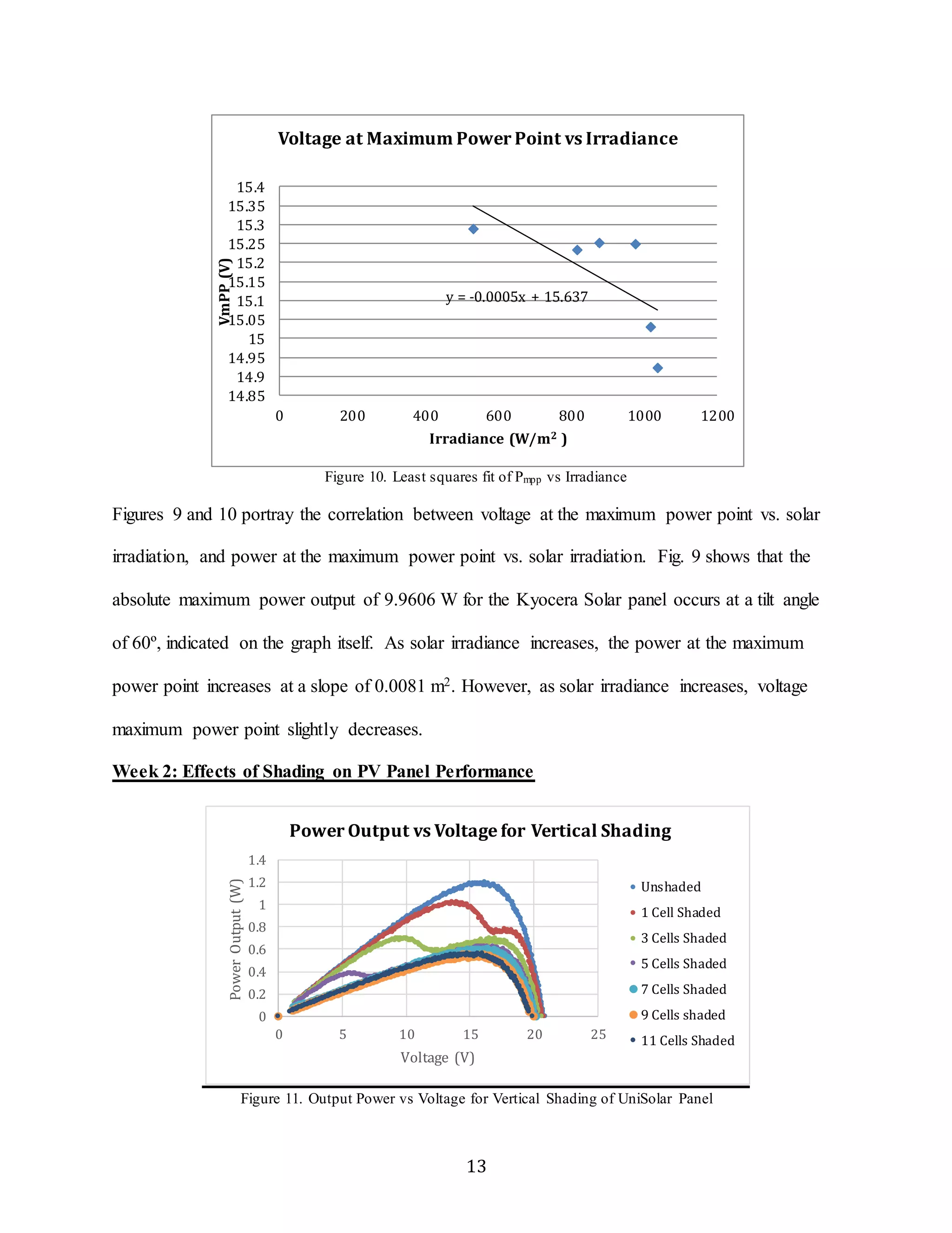
optimizing all factors (such as temperature and irradiance). Voltage should theoretically increase
with solar irradiance because more voltage would be generated when there is more irradiance.
However, Fig. 10 shows a negative relation between voltage and solar irradiance. This could be
explained by other factors affecting the actual voltage that was generated. The voltage decreases
at in extremely slight negative fashion, indicating that a small factor, such as a slight temperature
shift, could have switched the voltage from barely positive to barely negative.
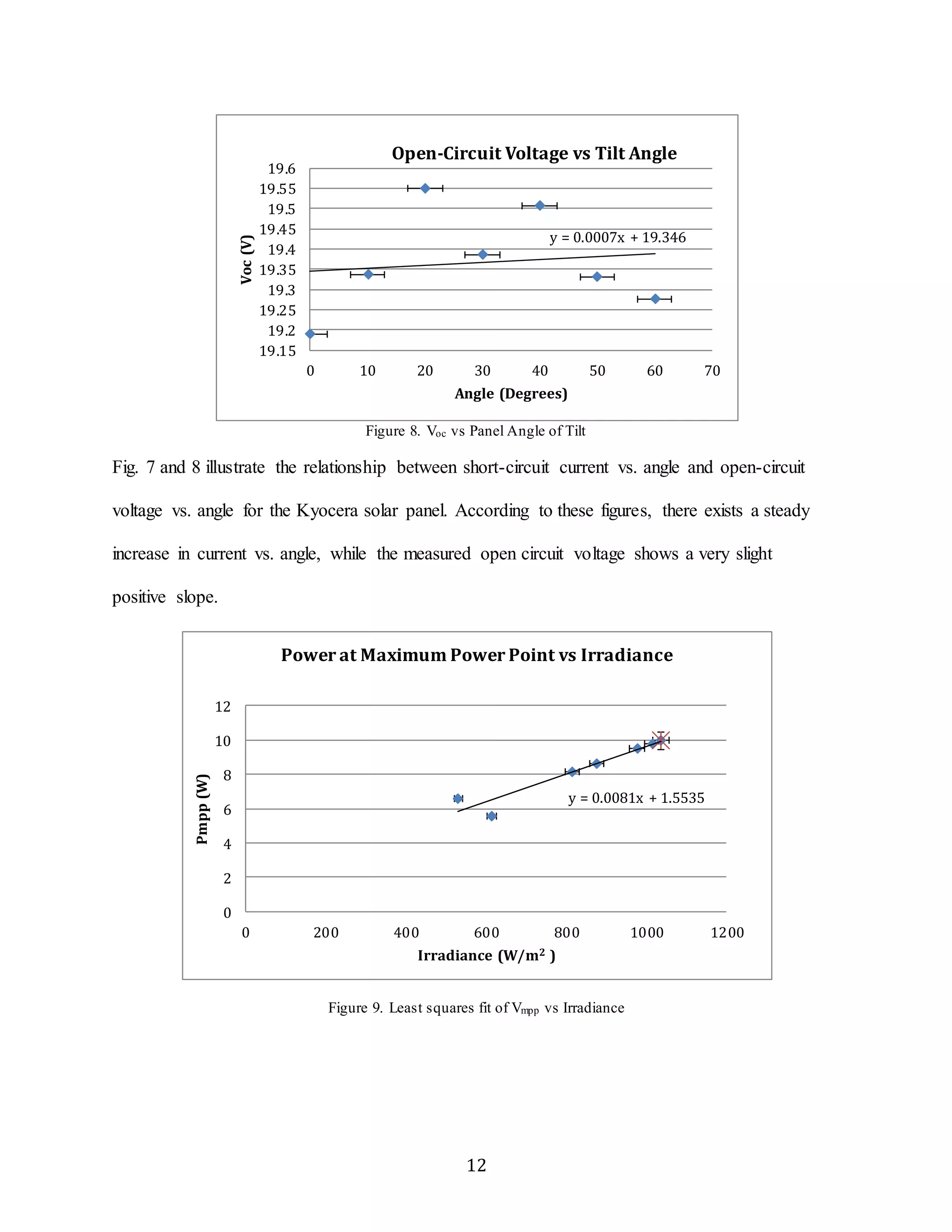
According to the Power at maximum power point vs. Irradiance curves, the maximum
panel power output occurs at an angle of 60 degrees, where irradiance is at the greatest. This
potentially can be attributed to the time of day the data was collected. Because it was late
afternoon, the sun had shifted from the highest point and came in at a lower angle, thus changing
the angle at which the highest irradiance would be observed. The maximum power point occurs

21. on the I-V curve where the curves transitions to a decreasing slope due to power being related to
21
voltage and current by P = IV.
While taking measurements at different angles, we needed to manually measure the angle
as well as hold the PV panel at the desired angle by hand. Due to these imprecise experimental
techniques the errors associated with PV panel angle are large, +/- 3 degrees. Another type of
error was having negative slope for Vmpp vs. Irradiance is due to application-related errors where
we might have accidentally changed the orientation of the sensors or not accounted for other
factors in the environment. The built in intrinsic errors within the M-170 sensor unit in the
measurement of voltage, current, power, and irradiance are negligible.
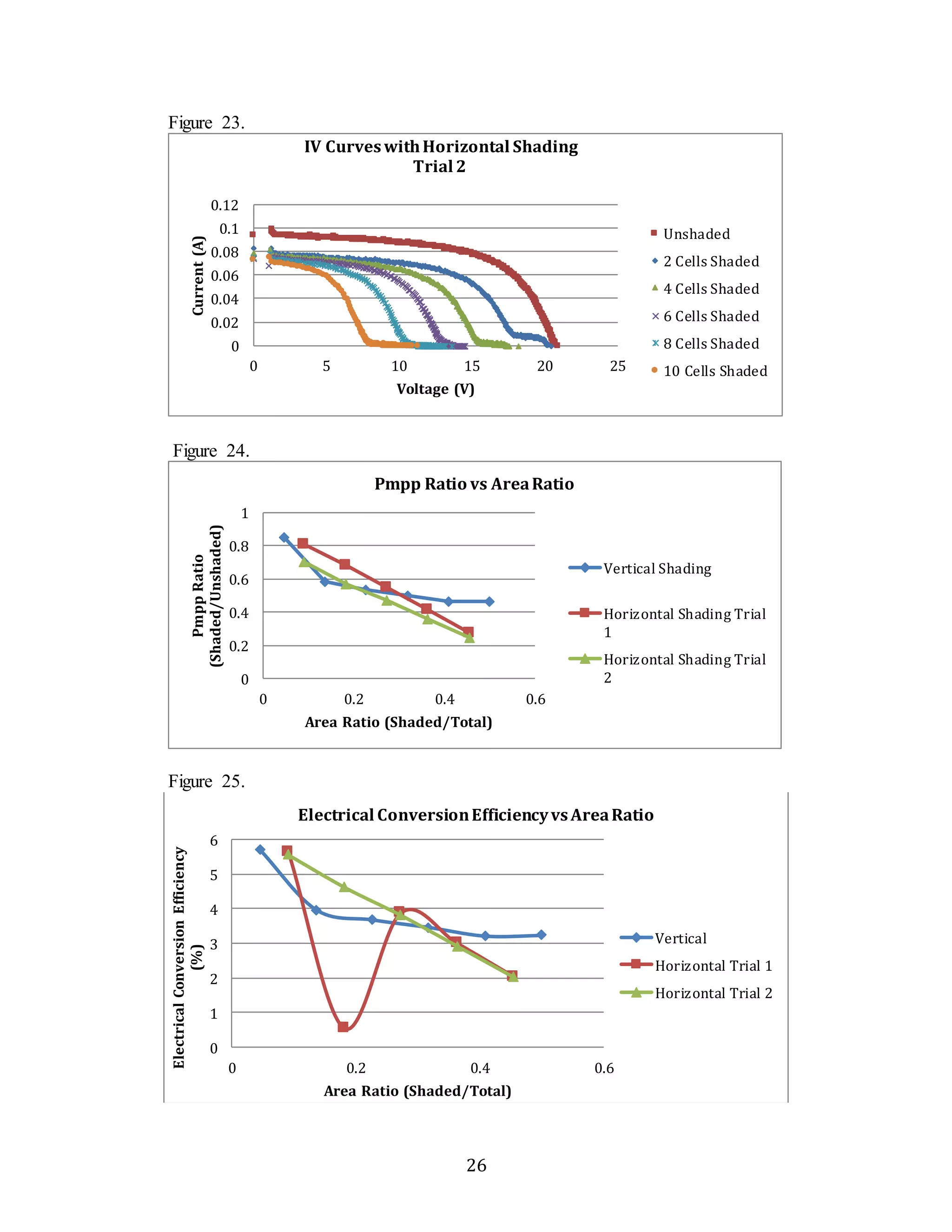
Week 2:
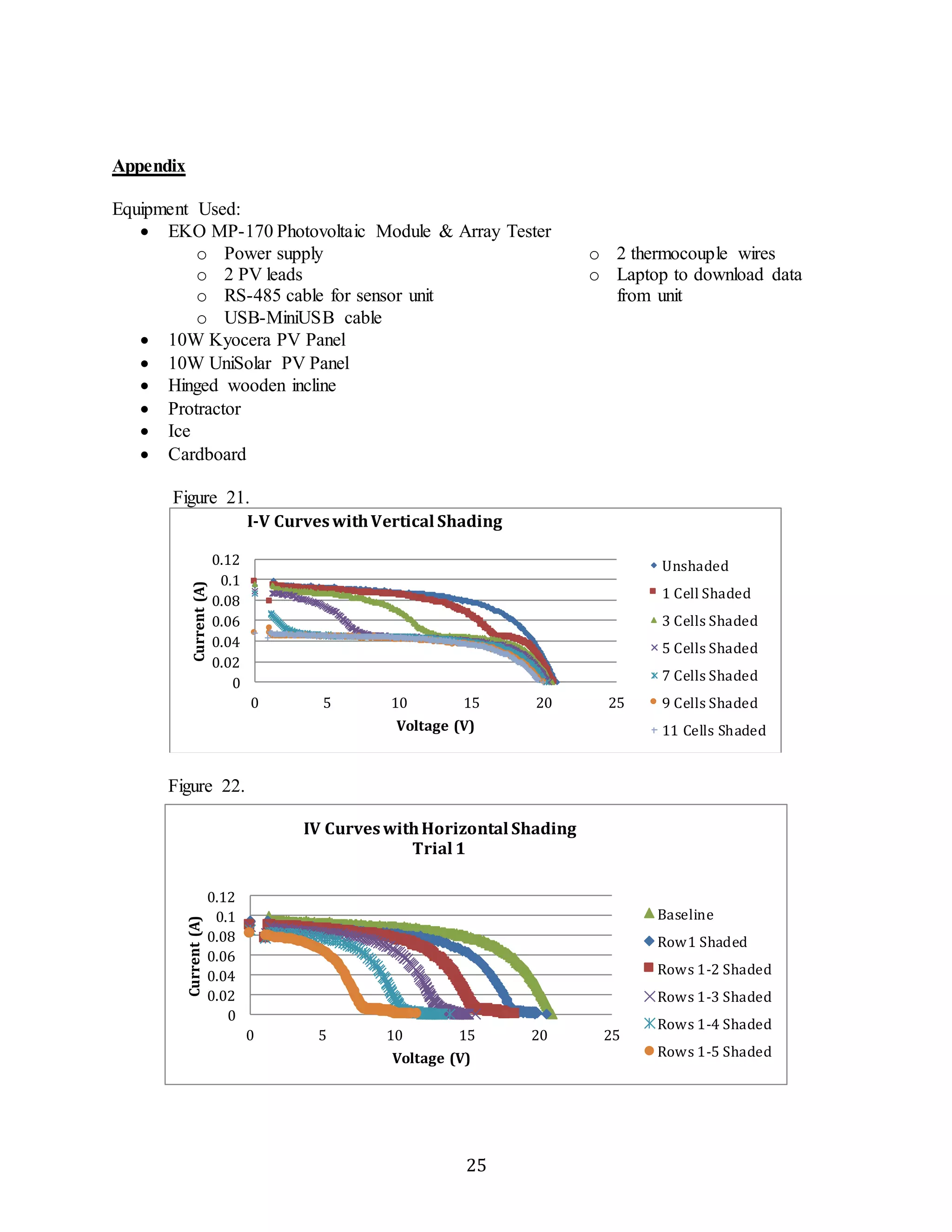
The results imply that PV systems are designed so as to maximize the power output even
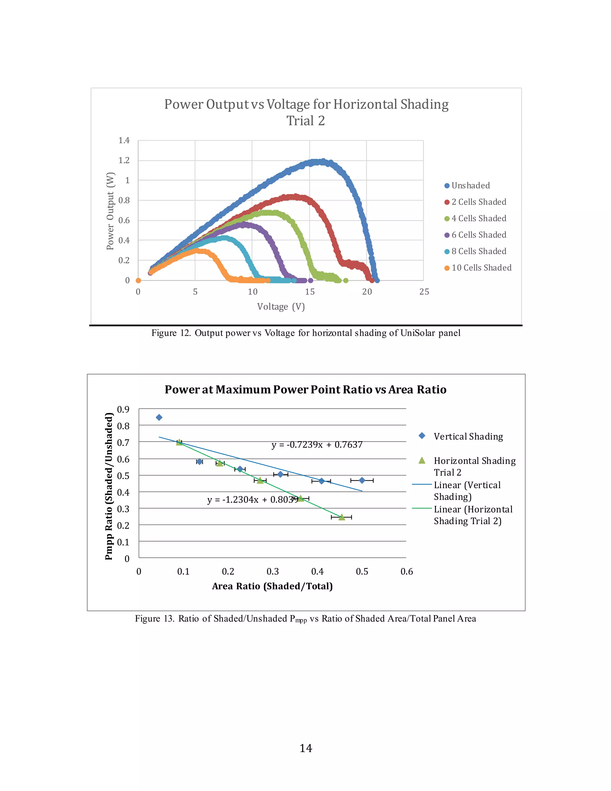
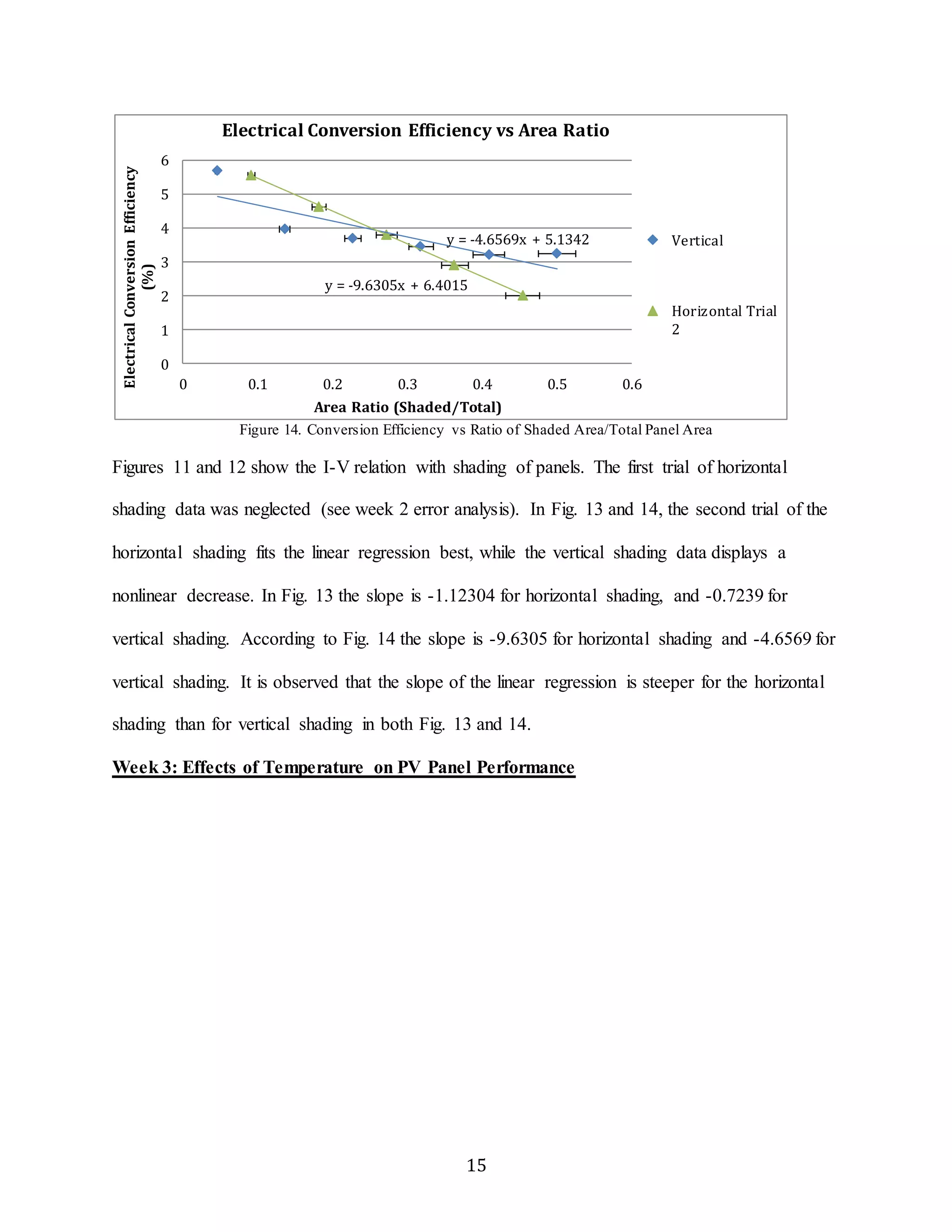
when shaded. The more rapid decrease in both power at maximum power point and electrical
conversion efficiency for horizontal shading compared to vertical shading (Figures [13, 14]) can
possibly be attributed to the way the individual cells of the PV panel are connected. While
vertically shading, only one cell in each horizontal module (group of two horizontal PV cells)
falls was shaded. That cell falls to a power output of zero, but the power output of the entire
module does not fall to zero. However, while horizontally shading, the entire module is covered,
and thus the entire power output of the full module falls to zero.4 In order to accommodate for
potential power losses due to shading, the PV system would have to be designed to minimize
coverage of full horizontal modules. To accomplish this, the rows of the PV panel could be wired
in series, while the columns could be wired in parallel. According to Ohm’s Law, the connection
in series would maximize output voltage, but would create power-draining loads when individual

22. cells are shaded. Thus, the parallel connection serves to create an equal distribution of voltage to
22
minimize the power loss due to shading.
The shading was produced by hand with a piece of cardboard. This imperfect technique
could have led to some imperfect shading. To account for this potential error, we assumed a 5%
error. This application related error was due to user interaction with the equipment. Further,
inconsistent irradiance from changing cloud cover affected the data significantly.
Week 3:
The experiment the relative trends between irradiance, temperature, and efficiency on a
PV panel. Theoretically, increased temperatures should lead to decreased efficiency in a PV
panel. However, other factors do play a significant role in affecting the efficiency. There is no
observable trend because of the different changing factors involved in the temperature-based
experiment. The data indicates a slight positive increase in electrical conversion efficiency and
voltage as temperature increases. However, the irradiance was extremely scattered throughout
the dataset, and therefore negates observable correlation between global irradiance and
efficiency. Shifting levels of irradiance due to cloud cover changed ambient air temperatures,
and thus disturbed the data sets. One possible reason for a positive increase in efficiency with
increased temperature is increasing irradiance at a higher rate than temperature. The corrected
electrical conversion efficiency indicates the true correlation between efficiency and
temperature, with a clear decrease in efficiency as temperature increases. Further complications
include water spillage on the solar panel. This not only increases the specific heat capacity, but it
cools down the panel, thus changing the correlative data. The trends for Impp vs Panel
Temperature and Corrected Impp vs Panel Temperature both have a similar positive behavior.

23. 23
Conclusion
This experiment has concentrated on the analysis of the relationship between solar panel
tilt angle, the effect of shading on solar panel performance, and the effect of temperature on PV
performance. The maximum power output for Kyocera solar panel was found to be 9.96W at the
tilt angle of 60º, where the solar irradiance has a positive correlation with power output. The
experiment had shown that horizontal shading had a more significant impact on power output
than vertical shading. The experiment also shows that temperature has a negative correlation
with electrical conversion efficiency. Changes in any factors affecting power output can
significantly change the result. Therefore, PV systems must be designed to accommodate a
balance between the least amount of horizontal shading, the most irradiance, and the least
possible panel temperature.

24. 24
References
1. "Solar Angles and Tracking Systems." Solar Angles and Tracking Systems - Lesson -
Www.TeachEngineering.org. N.p., 05 Feb. 2014. Web. 02 Feb. 2014.
2. "Part II – Photovoltaic Cell I-V Characterization Theory and LabVIEW Analysis Code." -
National Instruments. N.p., 10 May 2012. Web. 02 Feb. 2014.
3. Kleissl, Jan, and R. A. De Callafon. "Laboratory Course Website, Dept. of Mechanical and
Aerospace Engineering at UCSD." Laboratory Course Website, Dept. of Mechanical and
Aerospace Engineering at UCSD. N.p., 18 Feb. 2013. Web. 02 Feb. 2014.
4. “Solar Electronics, Panel Integration and Bankability Challenge.” GreenTechMedia.
http://www.greentechmedia.com/articles/read/solar-electronics-panel-integration-and-the-bankability-
challenge. 06 Feb. 2014.

25. I-V Curves with Vertical Shading
IV Curves with Horizontal Shading
25
Appendix
Equipment Used:
 EKO MP-170 Photovoltaic Module & Array Tester
o Power supply
o 2 PV leads
o RS-485 cable for sensor unit
o USB-MiniUSB cable
o 2 thermocouple wires
o Laptop to download data
from unit
 10W Kyocera PV Panel
 10W UniSolar PV Panel
 Hinged wooden incline
 Protractor
 Ice
 Cardboard
Figure 21.
0.12
0.1
0.08
0.06
0.04
0.02
0
Figure 22.
0 5 10 15 20 25
Current (A)
Voltage (V)
Unshaded
1 Cell Shaded
3 Cells Shaded
5 Cells Shaded
7 Cells Shaded
9 Cells Shaded
11 Cells Shaded
0.12
0.1
0.08
0.06
0.04
0.02
0
Trial 1
0 5 10 15 20 25
Current (A)
Voltage (V)
Baseline
Row1 Shaded
Rows 1-2 Shaded
Rows 1-3 Shaded
Rows 1-4 Shaded
Rows 1-5 Shaded

26. IV Curves with Horizontal Shading
Trial 2
Pmpp Ratio vs Area Ratio
Electrical Conversion Efficiency vs Area Ratio
26
Figure 23.
0.12
0.1
0.08
0.06
0.04
0.02
0
Figure 24.
1
0.8
0.6
0.4
0.2
Figure 25.
0 5 10 15 20 25
Current (A)
Voltage (V)
Unshaded
2 Cells Shaded
4 Cells Shaded
6 Cells Shaded
8 Cells Shaded
10 Cells Shaded
0
0 0.2 0.4 0.6
Pmpp Ratio
(Shaded/Unshaded)
Area Ratio (Shaded/Total)
Vertical Shading
Horizontal Shading Trial
1
Horizontal Shading Trial
2
6
5
4
3
2
1
0
0 0.2 0.4 0.6
Electrical Conversion Efficiency
(%)
Area Ratio (Shaded/Total)
Vertical
Horizontal Trial 1
Horizontal Trial 2

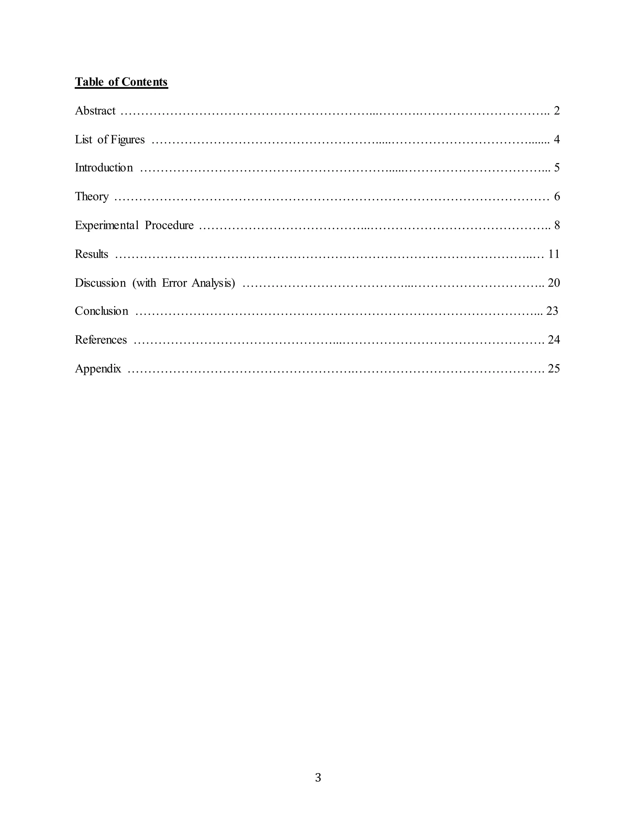
27. Current at Max Power Point vs Panel Temp
y = 0.016x - 0.0821
0 5 10 15 20 25
Temperature (°C)
27
Figure 26.
Table 1.
KY PV
Panel
0.5
0.4
0.3
0.2
0.1
0
-0.1
Current (A)
Solar
Irradiance
(Er)[W/m^2]
y = 0.0014x + 0.0708
Trial 1
Trial 2
Trial 1 Impp
Trial 2 Impp
PV Device
Temp.[degC] Isc[A] Voc[V] Pm[W] Ipm[A] Vpm[V]
Rated 1000 25 0.62 21.7 10 0.58 17.4
0 Degrees 614.415929 53.766987 0.413645 19.189079 5.589738 0.366618 15.246755
10
Degrees 530.923451 54.466408 0.488166 19.336191 6.589841 0.431026 15.288747
20
Degrees 814.993215 54.670582 0.59202 19.548725 8.123451 0.533357 15.230793
30
Degrees 875.20826 57.693634 0.633405 19.386742 8.58644 0.563004 15.251104
40
Degrees 977.099853 57.42136 0.7029 19.506508 9.532833 0.625251 15.246416
50
Degrees 1016.128024 60.871288 0.728513 19.330552 9.759039 0.649358 15.028747
60
Degrees 1036.060177 61.873493 0.744509 19.274462 9.960568 0.66762 14.919507