1. Ali Homayounfar
©
1
Table of Contents
List of Abbreviations .................................................................................................2
Abstract........................................................................................................................3
Keywords .....................................................................................................................3
Chapter 1: Literature Review and Introduction ..................................................4
1.1. The History of Euro and Euro-dollar Exchange Rate..............................................................4
1.1.1. When New Members Join the Euro Area..............................................................................5
1.2. Previous Research on the euro-dollar Currency.........................................................................6
1.3. Currency Manipulation by Governments ...................................................................................10
1.3.1. How China’s Currency Manipulation Affects the Global Market..............................11
1.3.2. How Manipulating a Currency Exchange Rate can be a Threat to that Country’s
Economy .....................................................................................................................................................12
1.4. Unexpected Events’ Impact on the Euro-dollar Exchange Rate.......................................14
1.4.1. 11 September 2001......................................................................................................................14
1.4.2. Lehman Brother Bankruptcy in August 2008....................................................................14
1.4.3. Afghanistan and Iraq war..........................................................................................................15
Chapter 2: Research Methodology....................................................................... 16
2.1. Research Question, Research Hypothesis, Aims and Objectives......................................16
2.1.1. Aims and Objectives...................................................................................................................16
2.1.2. Research Hypothesis...................................................................................................................17
2.1.3. Research Question.......................................................................................................................17
2.2. Research Methodology for Economic Indictors and Demographic Factors
Influencing the Exchange Rate .................................................................................................................18
Chapter 3: Statistical Data Analysis and Results............................................... 22
3.1. Average and Standard Deviation ofa Year Calculated from the Daily Data of Euro-
dollar Exchange Rate.....................................................................................................................................22
3.2. The Impact of Gross Domestic Products on the Exchange Rate.......................................24
3.3. The Consumer Price Index inside the eurozone and USA...................................................30
3.4. Government Debt as a Percentage of GDP in the Eurozone and USA...........................34
3.5. Analysis ofMarket Currency After a Daily Shock .................................................................37
3.6. Increase of Oil Prices and US Budget on Wars.........................................................................41
3.7. Demographic Factors and unemployment rate.........................................................................43
3.7.1 Young Working-age Population Rate....................................................................................43
3.7.2 Governments’ Policies on Immigration and Intervention in the Market....................48
Chapter 4: Conclusions and Recommendations................................................ 50
4.1. Conclusions................................................................................................................................................50
4.2. Future Works ...........................................................................................................................................53
References ................................................................................................................ 54
Appendix A1. Data Range from max of EUR/USD to min of EUR/USD...............................60
Appendix A2. CPI-ratio vs. EUR/USD..................................................................................................61
Appendix A3. Government Debt Ratio vs. EUR/USD....................................................................61
Appendix A4. Testing the Output of the MATLAB Algorithm.................................................62
Appendix A5. Unemployment Ratio in the EU and Euro Area .................................................62
Appendix A6. Member States of EU and the Year of Entry........................................................63

2. Ali Homayounfar
©
2
List of Abbreviations
ARIMA: Auto-Regressive Integrated Moving Average
BEER: Behavioural Equilibrium Exchange Rate
CP: Consumer Price
CPI: Consumer Price Index
ECB: European Central Bank
EEC: European Economic Community
EMU: Economic and Monetary Union
ERM: Exchange Rate Mechanism
EU: European Union
EUR: Euro
GDF: Government Debt Fraction
GDP: Gross Domestic Product
GOF: Government Obligation Factor
RMB: Renminbi
USA: United States of America
USD: United States Dollar

3. Ali Homayounfar
©
3
Abstract
The aim of this dissertation is to investigate and to expand on the previous research on
the euro-dollar exchange rate from 1999 to 2012. Some government policies such as
currency manipulation and their influence will also be discussed.
By using a methodology based on statistical data analysis, correlation and regression
analysis, the relationship between the US dollar and the euro according to the
economic indictors such as consumer price index (CPI), gross domestic products
(GDP), government debt in the eurozone and the USA will be analysed.
Unexpected events and incidents, for example the 2008-2009 global economic turmoil
impacted on the euro-dollar exchange rate; this caused unstable daily exchange rate,
our aim is to find a new model to see to what extent this model can predict the
exchange market for a short period, e.g. up to 10 days after a sudden one-day shock
happens to the currency.
Some analysis of the most important demographic factors such as the birth rate and
death rate in the European Union, eurozone and United States of America will be
discussed; and an attempt to establish the relationship of those demographic factors to
the unemployment rate and the immigration rules of respective governments will be
made.
Keywords
Euro-dollar exchange rate, consumer price index, gross domestic product, government
debt, Eurozone, unemployment rate, demographic factors

4. Ali Homayounfar
©
4
Chapter 1: Literature Review and Introduction
1.1. The History of Euro and Euro-dollar Exchange Rate
The euro was officially adopted on 16 December 1995 by the Madrid European
Council 15 and 16 December Presidency Conclusion, and the European Council
adopted the euro to be introduced to the world as a currency on the first day of 1999.
According to the European Central Bank (ECB), today 18 out of 28 of countries of the
European Union use the euro as their currency. Since the euro was launched in 1999
at the exchange rate of 1.1743 vs. US dollar, the pattern of the euro against the dollar
is still an interesting topic for research, as the behaviour is still not completely
understood.
The European Central Bank’s task is to provide the purchasing
power for the euro and stability inside the eurozone.
There are six important dates in euro history: when the 18 European
countries joined the euro area, on 1 January 1999 for Austria, Belgium,
Finland, France, Germany, Luxembourg, Ireland, Italy, the Netherlands,
Spain and Portugal; 1 January 2001 for Greece; 1 January 2007 for Slovenia; 1
January 2008 for Cyprus and Malta; 1 January 2009 for Slovakia; 1 January 2011 for
Estonia; and 1 January 2014 for Latvia.
Joining countries with lower Gross Domestic Product (GDP) and higher
unemployment rates to the eurozone will be discussed in section 1.1.1 to discover
how this affected the euro’s strength compared with the US currency.
According to ECB, today the US dollar and euro take respectively 62% and 25% of
reserve currencies. Since the launch of the euro in 1999 the US dollar had a drop of
10% (from 72% to 62%) and the euro had a rise of 7%.
The US dollar is also being used officially in some countries such as East Timor,
Ecuador, El Salvador and also unofficially in countries with a
significantly weak economy.

5. Ali Homayounfar
©
5
Let’s define the euro to US dollar exchange rate as a fraction of one euro in terms of
the dollar, EUR/USD; in this dissertation every time we refer to EUR/USD or EUR to
USD, we mean that fraction. For example, referring to a daily currency rate as
EUR/USD =1.25 indicates that 1 euro is equivalent to 1.25 USD on that date. The
data for calculations and modelling are collected from the World Bank unless
mentioned that the data are collected from other sources such as the European Central
Bank (ECB).
1.1.1. When New Members Join the Euro Area
From January 1999, 11 of the economically developed European countries of the 15
members of the EU adopted the euro as their currency; however Greece, because of a
weaker economy, did not join the euro area until 2 January 2001. Still after 15 years,
the UK, Denmark and Sweden have decided to not join the eurozone. From 1 January
1999 to 19 July 1999, although the euro-dollar rate was slightly volatile, the euro’s
strength against the dollar reduced gradually from EUR/USD = 1.1789 to EUR/USD
= 1.0146. Since 19 July 1999 to 26 October 2000, the volatility increased but still the
euro continued losing strength until 26 October 2000 with a rate of EUR/USD =
0.8252, which is the lowest euro rate in the history of the euro up to now (November
2014). However, from 2002 to 2008 the euro started to become strong significantly.
On 15 July 2008, EUR/USD =1.5990, which has been the highest rate in euro-dollar
history. After that time, up to today, the euro-dollar exchange rate became more
volatile than before and in some cases the euro lost its strength against the dollar. This
could be due to the effects of the global financial crisis, weak economy and high
unemployment rate in some euro states (Riley, 2013) especially Greece and Spain and
other new states joined the eurozone with a much lower GDP compared to old
members.
Therefore, it can be concluded that in the first year of the euro, due to adopting a new
currency in 11 countries, the euro market was not stable enough. After that, because
of some reasons that will be discussed in the following sections, the euro became
stronger until the start of the global turmoil in 2008 and 2009.

6. Ali Homayounfar
©
6
The days before and after the date that Greece and Slovenia respectively joined the
eurozone on 1 January 2001 and 1 January 2007, there were not any drops in the euro
against the dollar. This can be due to the stronger days of the euro compared with the
USD; the countries with a lower GDP and higher unemployment rates that joined the
eurozone could not depreciate the euro against the dollar.
On the days after 1 January 2008, 1 January 2009, 1 January 2011 and 1 January
2014, Cyprus and Malta, Slovakia, Estonia and Latvia respectively joined the euro
area and the euro-dollar exchange rate dropped by -0.2%, -0.4%, -0.1% and -0.15%.
This can be for the period of weakness of the euro. However all of these depreciations
were for only one or two days, which cannot be considered as a main factor of strong
volatility of the euro-dollar rate.
1.2. Previous Research on the euro-dollar Currency
Heimonen (2009) presented results for equity flows between the Economic and
Monetary Union (EMU) and the USA, and their impact on the EUR to USA exchange
rate. He explained that the excess of the eurozone’s equity returns over USA’s equity
returns causes an equity flow from the eurozone to USA. When residents of eurozone
countries purchase US equities, this causes increases in the price of the USD against
the euro; and when US residents buy the eurozone’s equity, this follows by
appreciation of the euro against the dollar.
Heimonen also presented a model by taking into account both exchange rate and flow
equations; its result mentioned that eurozone equity returns have more significant
performance in euro-dollar pattern than US equity returns. Heimonen also stated that
the value for equity flow has increased sharply since 1999. There are some classical
models such as the behavioural equilibrium exchange rate (BEER) to estimate the
euro-dollar exchange rate, which indicates that the equity market can have a
significant effect on the equilibrium value for the exchange rate (Heimonen, 2009).
However, to the best of our knowledge, since 1999 due to many important and
unpredicted factors with the equilibrium model, nobody could present an accurate
model for the equilibrium.

7. Ali Homayounfar
©
7
Purchasing power parity (PPP) is another conventional model to predict equilibrium
exchange rate; however Sarno and Taylor (2002) and Detken et al. (2002), after
research on empirical results by some evidence, proved that PPP might not be an
essential factor to affect relations between the euro and the dollar.
In some cases incorporation between PPP and the bond market shows their effects of
the long-run equilibrium exchange rate (Juselius and MacDonald, 2000; 2004).
However, other research states (Heimonen, 2009) that the equity market does not have
a strong influence on the equilibrium exchange rate, although the equity market has
increased sharply in recent years.
Unlike the debt flow, the flows for equity portfolio play a more important role than
bond market on exchange rate; this might be due to the fact that the equity portfolio
flows are not usually hedged (Heimonen, 2009). In the early years of the 2000s
Maeso-Fernandez, Osbat and Schnatz (2001) described that the exchange rate is under
a high influence of productivity and oil price; however there was not enough proof for
this research. Hence one of our goals in this dissertation will be to analyse how the
increase in the price of oil from 2001 and its impact with the GDP of the USA and
eurozone will influence euro-dollar exchange rates.
In addition, Feroli (2006) proved that demographic factors until 2005 such as net
migration and rates for birth, death and unemployment of a country can influence the
current account balance; this will be mentioned further in the following chapters as
one of the aims for the dissertation, from 1999 till 2012. Unlike Feroli (2006), Tille,
Stoffels and Gorbachev (2001) could not find enough evidence for the influence of
ageing for the US dollar vs. the eurozone in 2001; however they found enough results
for the US dollar vs. the Japanese yen. In our work, it is a chance after twelve years
since introduction of euro 1999 and new members joining the eurozone, which mostly
have lower GDP than old members of the EU, to investigate whether or not there is an
impact of ageing for the exchange rate in the USA vs. the eurozone. In this report we
will also try to take into account some other political factors such as government
policies on immigration and war on terror.
Cohen and Loisel (2001) mentioned that currency depreciation is due to many
restrictive fiscal policies in the euro states.

8. Ali Homayounfar
©
8
Alquist and Chinn (2002) demonstrated that dollar appreciation is due to the high
level of US productivities; however Schnatz, Vijselaar and Osbat (2004) rejected that
theory by explaining that they did not discover enough documents and other
influential factors that might dominate the effects of productivity on the exchange rate
in recent years.
In the first years of after establishment of the euro, Sinn and Westermann in 2001
suggested that the weakness of the euro is because of the shift in alterative currency
balances from the German mark to the dollar inside transition countries (Germany,
France, Italy and Spain play the most important roles in world economics in terms of
GDP and also in G6 and political matters such as the war on terror and demographic
factors that affect immigration), whilst Meredith (2001) linked this to portfolio shift,
caused when borrowers issue euro debt and shifted by lenders towards non-euro
assets. However, Gómez, Melvin and Nardari (2007) explained euro weakness due to
the fact that market participants were first learning low inflation policies in the
European Central Bank.
Cheung and Chinn (2000) proved the impact of economic parameters shift over time
whilst Goldberg and Frydman (2001) and Frömmel, MacDonald and Menkhoff
(2005) stated the time dependency could be linked to the exchange rate model.
It is important to note that conventional exchange rate models cannot explain the
behaviour of the euro-dollar exchange rate anymore today. Since the middle of the
1990s the equity flow has increased (Lane and Milesi-Ferreti, 2003; 2004) whilst
research states that the exchange rate, especially dollar-euro, relates to the equity
market (Heimonen, 2009).
The foreign direct investment and portfolio equity increased and related to
international debt stock (Lane and Milesi-Ferreti, 2003) such as bonds. In the first
days of the establishment of euro, appreciation of the dollar had a direct relation with
US stock; hence it was concluded that the stock market could have a relation to the
exchange rate; which can be calculated from fund flow to the stock market (Bailley
and Millard, 2001; Brooks et al., 2001).

9. Ali Homayounfar
©
9
It is obvious that increasing the flow of funds has a direct relationship with equity
prices followed by an increase in consumption, investment, demand and capital stock
and productivity.
Portes and Rey (2005) presented a correlation between domestic and foreign equity
returns reducing equity flows; they also indicated that amounts of trade and domestic
equity markets are essential factors for equity flows.
In addition, Hau and Ray (2004; 2006) stated that the short-run relationship between
equity return and exchange rate is negative. They also indicated that increasing
foreign equity to the home equity causes portfolio balancing, making home investors
reduce their foreign equity to reduce the exchange rate (in other words to increase
domestic currency strength).
In addition, Cappiello and DeSantis (2005) proved that the larger equity returns in a
country cause more depreciation of its currency; however if issues of stocks influence
equities, there will be no relation between the return of equity and the exchange rate
(Sinn and Westermann, 2001).
On the other hand, Pavlova and Rigobon (2003) indicated that the variation between
the equity market and the nominal exchange rate are related to the type of shock,
which can be a positive or negative relationship due to the type of the shock.
Pavlova and Rigobon (2003) also used an international asset-pricing model that states
the influence of positive shock (by considering other conditions remaining the same)
to a country’s output leads to reducing the trade and depreciating the exchange rate.
On the other hand the demand shock follows by appreciation of the exchange rate.
The demand shock as a short-run influence and supply shock as a long-term influence
on markets is presented by Pavlova and Rigobon (2003) as a conventional equilibrium
exchange rate model, indicating effects of productivity on the real exchange rate.
Weisang and Awazu (2008) used three auto-regressive integrated moving average
(ARIMA) models by using macroeconomic indicators to model the euro/dollar
exchange rate. They discovered that the monthly euro/dollar exchange rate is the best
model by using a linear relation between its past three values and the current and past

10. Ali Homayounfar
©
10
three values of the difference of the log-levels of the share price indices between the
euro area and the United States.
Chinn and Frankel (2008), using econometric calculation, predicted that the euro in 10
to 15 years will surpass the dollar. Their prediction was based on fundamental factors
that economists generally consider, such as economic size in trade, the liquid and
developed financial market and network externalities; they also forecast that new
members of the euro area will increase the GDP of the eurozone significantly to
influence the GDP of the US. Chinn and Frankel in 2008 explained that the euro has a
much higher potential rival than the Deutsche mark and the Japanese yen used to
have; they also explained that the US for more than two decades has had unstable
current account deficits, hence they concluded that between 2015 and 2024 the euro
will surpass the USD in terms of its trade invoicing role and vehicle currency role.
Similar arguments were presented by other financial analysts such as Papaioannou
and Portes (2008). As mentioned in section 1.1.1, during 2003 to 2008 there was a
period of appreciation of the euro against the dollar, hence euro-optimist economists
made their arguments based on that period; however, as it will be discussed in the
following sections, after 2008 the eurozone, like the USA, suffered from crises such
as increasing government debts and increasing unemployment rates. In 2009, after
sudden deprecations of the EUR to the USD, De la Dehesa (2009) presented some
challenges that the euro must face against the dollar as three categories in the financial
market: 1- the international asset management market; 2- the foreign exchange
market; and 3- the international liability management market.
As mentioned above, there have been various kinds of research and quantitative
model analysis for the essential factors of the euro-dollar exchange rate in the last
decade. However, as it was also explained, that research was in many aspects
controversial due to conclusions of different groups either to support or reject
different hypotheses regarding what are the main factors to influence the exchange
rate. In chapters 2 and 3, we will explain some novel methods that can be less
controversial than other previous works that have been done.
1.3. Currency Manipulation by Governments

11. Ali Homayounfar
©
11
Sometimes a government of a country might revalue its currency by pushing it
towards appreciation (depreciation) to achieve more imports (exports) and fewer
exports (imports). In the following section two of the most famous cases, China in
recent years and Black Wednesday in the UK in 1992, will be discussed.
1.3.1. How China’s Currency Manipulation Affects the Global Market
In recent years, China has prevented its currency from appreciating in markets to
make more exports and fewer imports. This makes China’s exports less expensive and
its imports more expensive than they should be. In other words China’s policy
encourages other countries to import more goods from China while the Chinese are
discouraged to import from other countries. This affects other countries’ economies
such as job losses in the US, and several bills have been introduced to US congress
regarding the undervalued currencies (Morrison and Labonte, 2013). This might raise
political issues as a threat to the US and China’s relationship and other global trading
countries involved (Ikenson, 2010).
Meanwhile China is buying US (Labonte, 2012) and European assets and securities
(Godement and Parello-Plesner, 2001), which are an alternative way in future if the
crisis in the Chinese market Renminbi (RMB) cannot be controlled by the Chinese
government any more, so China, by selling foreign assets, can use an alternative way
to control the RMB against collapse.
Hence, this brings an argument (Ikenson, 2010) among politicians to discuss that if
the US government puts pressure on China to stop manipulating its currency to avoid
extra exports from China to the US and fewer exports to China from US, then China
might stop buying US assets and securities (Labonte, 2012).
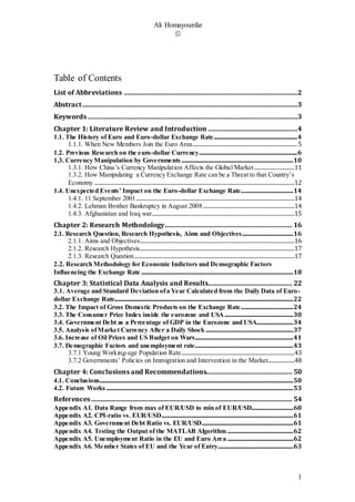
From July 2005 to July 2008 when the euro had appreciated against the USD
continuously (from a mean of EUR/USD=1.24 in 2005 to a mean of EUR/USD=1.47
in 2008), the Chinese central bank monitored the RMB to also be appreciated against
the dollar by around 21% (the RMB/USD increased from 0.12 in July 2005 to 0.145
in July 2008); this caused Chinese products which had been sold to Europe and the
US to become more expensive than their real values of RMB. From July 2008 due to
the global turmoil, China prevented further appreciation of its currency to help

12. Ali Homayounfar
©
12
countries in crisis to continue buying from China. From July 2008 till mid June 2010,
the Chinese yuan was kept almost constant at the RMB/USD for 0.145, which
followed more Chinese exports to the US and Europe, and fewer exports from other
countries with a strong currency to China. Figure 1 exactly shows the details
mentioned above, when the Chinese currency had a sharp rise from 2005 to 2008 and
then almost had a constant value from 2008-2010.
Figure 1. Chinese yuan in terms of US dollars (RMB/USD) for each year of 1999 to 2012
Although China allowed the rate for RMB/USD to rise in November 2011 to 0.157,
US officials still criticised the Chinese currency rate increase for being too slow.
1.3.2. How Manipulating a Currency Exchange Rate can be a Threat to that
Country’s Economy
One of the best examples of this is ‘Black Wednesday’ in 1992, when Britain was
forced to withdraw sterling from the exchange rate mechanism (ERM).
In 1969 in Hague, the six original members of the European Economic Community
(EEC), Belgium, France, Italy, Luxembourg, the Netherlands and West Germany,
launched an agreement for EMU. Ireland, Denmark and the UK joined the EEC in
1972. To reduce the volatility among European currencies in 1979 the EEC
governments established an ERM; while the UK did not join at the ERM at that time,

13. Ali Homayounfar
©
13
it did so in 1990. In 1991, the governments of the European Union signed the
Maastricht Treaty for the EU and committed themselves to the EMU; however British
prime minister at the time, John Major, decided to stay out.
On Wednesday, 16 September 1992, due to the fact that the UK could not keep
sterling above its agreed lower limit, Britain was forced to withdraw the currency
from the ERM; it is important to take into account George Soros’ hedge fund on
Black Wednesday (Litterick, 2002; Leftly, 2012; Martin; 2012).
George Soros established Quantum Fund in 1972, which became one of the most
influential first hedge funds. According to Forbes (2014) today Soros is the twenty-
fifth wealthiest billionaire in the world and the third wealthiest in the investment
division.
In 1992, George Soros noticed that sterling has been overvalued due to the fact that
British pound was pushed into ERM at too high a rate. He noticed that, as the British
Conservative Party government was under heavy pressure, that in the near term future
either the UK would have to withdraw from ERM, or sterling would have to be
revalued.
Soros borrowed around £6.5 billion and swapped it to other European currencies such
as French francs and German marks (Deutsche mark). On the days following ‘Black
Wednesday’ Soros paid back his original borrowings and profited by around £1
billion. Soros also bought around £350 million in shares as he expected that a
country’s equities often rise after the devaluation of that country’s currency.
Treasury documents released under the Freedom of Information Act in 2005 revealed
the total losses from Black Wednesday amounted to £3.3 billion (HM Treasury, The
national archives, 2005).
However the prime minister and chancellor at the time, John Major and Norman
Lamont, both explained that the losses of Black Wednesday were dwarfed when
compared to the overall state of the economy.
Today, two decades after Black Wednesday, global turmoil in 2008-2009 and finally
the euro crisis recently, still suggests an argument about whether or not government

14. Ali Homayounfar
©
14
should restrict policies to avoid speculators doing the same as Gorge Soros’ hedge
fund did (Martin, 2012).
1.4. Unexpected Events’ Impact on the Euro-dollar
Exchange Rate
1.4.1. 11 September 2001
September 11 was one of the most unexpected events in market history in all aspects.
Although the terrorist attack caused one of the worst days of the US economy, on that
date the euro dropped by -0.9 percent from the previous day of 10. From 6 September
2001 to 17 September the euro appreciated against the dollar every day except a
depreciation of -0.9% on September 11 (from EUR/USD = 0.9047 on 10 Sep to
EUR/USD= 0.8964 on 11 Sep). Hence the euro currency market shock was higher
than in the US. This might be due to the strong tight economic relationship between
the euro area and the USA (Cooper, 2014).
Therefore, in the worst unexpected events for a country, a disaster shock cannot
always have negative impact on the currency of that country.
1.4.2. Lehman Brother Bankruptcy in August 2008
Lehman Brothers is one of the most important unexpected events that most finical
analysts refer to. Although this investment service and banking headquarters was
located in New York, its bankruptcy and other US crises in that period of time had
one of the fastest declines of the euro currency against the USD in a short period of
time, from EUR/USD = 1.4825 on 22 September 2008 to EUR/USD =1.2328 on 28
October 2008.
Therefore, once again it was proved that during a strong relationship of the US and
the eurozone the financial crisis in the US could cause as chaotic a time in the euro
area as the US.
For example, during the financial crisis in the USA, from 2008 to 2009, EU exports to
the USA dropped by 30% from 367.6 billion USD to 281.8 billion USD. However,

15. Ali Homayounfar
©
15
EU exports and imports in 2012 to the US were 380 billion USD and 265.1 billion
USD respectively (Cooper, 2014).
1.4.3. Afghanistan and Iraq war
On 7 October 2001, the US war on terror started in Afghanistan; however on 8
October the dollar appreciated against the euro; after two weeks the dollar depreciated
by -2 percent. A similar pattern was observed after 20 March, the start date of the Iraq
war; the day after the dollar had a very minor rise but after a week the USD had a
drop of -1 %. However these depreciations were not followed continuously in the
short term. Effects of war on the drop of dollars were gradual in the period of 2001 to
July 2008, which will be discussed in chapter 3.

16. Ali Homayounfar
©
16
Chapter 2: Research Methodology
2.1. Research Question, Research Hypothesis, Aims and
Objectives
2.1.1. Aims and Objectives
The first objective is a discussion of the correlation of the three essential economic
indicators, GDP, CPI and government debt, on the euro-dollar exchange rate. Then, if
any of those indicators have a correlation with EUR to USD, we will discover a model
or formula between that indicator and EUR/USD.
The other aim is an investigation of unexpected events’ impact such as war in the
Middle East and the global crisis in 2008 and 2009 on the volatilities of the euro-
dollar exchange rate. In other words, this involves an examination of how those
events influence the volatility of the euro-dollar exchange rate graph.
The other objective will be a novel analysis of a sudden daily growth/fall of the
exchange rate, and to examine a model to forecast market stability for a short term,
e.g. up to 10 days.
We should also investigate to what extent US government and EU policies on
immigration had an impact on job opportunities. Alternatively we may ask if it is
possible to find a correlation between the euro-dollar exchange rate and
unemployment rate, which is related to US and European economic policies since the
birth of the euro. This will achieve a novel analysis of the years between 1982 and
2011 to develop a further research agenda, drawing on issues such as demographic
factors and how government policies in the EU and the USA have influenced the
unemployment rate. In addition, previous works on demographic factors, as
mentioned in the literature review, usually run to 2006; hence we should continue this
field of research until the end of 2011.
By considering both the death rate and the working-age rate (the 16-year-olds who
join the labour force) and taking into account the unemployment rate, in what extent

17. Ali Homayounfar
©
17
increasing the elderly population and increasing (or decreasing) the young population
is a threat for a country?
2.1.2. ResearchHypothesis
It is also important to develop a hypothesis regarding whether or not there is a
relationship of an economic indicator with the EUR/USD exchange rate. We have
chosen three of the most essential economic indicators as GDP, CPI and government
debt. For example, by using linear regression methodology we can find out whether or
not the increase (or decrease) of the GDP of the eurozone as compared with that of the
USA, (GDPEurozone/GDPUSA), between 1999 and 2011 had a direct relationship with
the appreciation (or depreciation) of the euro against the US dollar. Our null
hypothesis is that there is no relationship between GDPEurozone/GDPUSA and
EUR/USD. Our alternative hypothesis is that there is a relationship between
GDPEurozone/GDPUSA and EUR/USD. By using the methodology as the linear
regression statistical analysis of economic indicator and EUR/USD, we can develop a
function of EUR/USD in terms of GDPEurozone/GDPUSA by implementing the Excel
data regression Analysis Toolpak.
Similar methods will be used for the demographic factors model we have developed.
Further details of our model will be presented in section 2.2 and Chapter 3.
The other hypothesis is whether or not our model suggests that in a short period the
market corresponds to fall/rise behaviour after the highest daily rise/fall change in
EUR/USD. An alternative hypothesis suggests a correlation between market
behaviour after each daily large shock with the rise/fall of that date, while the null
hypothesis suggests no correlation.
2.1.3. ResearchQuestion
It should be discussed whether it is possible to find a model or formula to correlate the
yearly changes in indicators, for example GDP, for appreciation or depreciation on
EUR/USD?

18. Ali Homayounfar
©
18
As we explained in section 1.3, due to export and import polices of some countries,
such as China, a government can manipulate the currency against further appreciation
or depreciation, while investors and hedge fund companies, by taking into account
many factors, e.g. account balance of that country, try to find a model to estimate how
much the country’s currency is manipulated. We try to examine if there is a novel
simple model to calculate this range of Chinese currency manipulation.
The other research question is whether by taking into account the past market
behaviour patterns during the daily shock, there is a model to predict the behaviour of
the currency market in a short period after each sudden daily appreciation or
depreciation of the euro against the dollar?
2.2. Research Methodology for Economic Indictors and
Demographic Factors Influencing the Exchange Rate
The statistical data and regression analysis will be the research methodology used for
this dissertation. By using regression from data analysis of the Excel Toolpak, we can
find out how our hypothesis is valid. First, we have to import two sets of data, for
example the first set of data is the annual GDP-ratio of eurozone to USA, and the
second set of data is the annual average value of EUR/USD; the Excel Toolpak
calculates the R for the two sets of data, and the closer R to 1, the better the regression
line on the data used, and the higher the correlation between the two sets of data. To
test if our results are statistically significant (reliable), we should check at
“Significance F”. If Significance F<0.025, the results are reliable, otherwise it is
better not to consider the results for the two sets of data.
In Chapter 3, to find a correlation between an economic indicator and EUR/USD, if
the R value is close to 1 and significance F<0.02, we will accept the alternative
hypothesis as a correlation between the economic indicator and EUR/USD; and we
will reject the null hypothesis as no correlation.
Until May 2013, The World Bank presented the data for economic indicators and
demographic factor up to the end of Dec 2011.
One of our first aims is to compare the GDP for each year from 1999 to 2011 for both
the euro area and the USA, then by using the average and median of the euro-dollar

19. Ali Homayounfar
©
19
exchange rate for each year, it is possible to discover to what extent the exchange rate
between the eurozone and the USA relied on their GDPs.
Generally it can be said that higher GDP causes larger income for a country. When
GDP of a country increases, this might be due to more export demands and fewer
imports (a positive balance of trade for that country), and spending more on domestic
products in USA (or in the euro area) rather than foreign products increasing dollar
(euro) appreciation.
By having a higher GDP the saving can increase which leads to reduction of foreign
debt and causes further appreciation of the exchange rate. However, dollar
depreciation against the euro after 2003 might have had an increase of US exports to
the world and lower imports from the EU; this followed by increasing the GDP of the
USA in most cases. In addition, as mentioned in the literature review, during
depreciation of a currency, foreign investors start buying that country’s equity for
future (when their home currency depreciates to shift back those purchased equities to
their home countries). Hence all these cause some equilibrium rates for volatility for
the exchange rates. Therefore, in this dissertation, an additional analysis should be
used to discover to what extent GDP growth inside the eurozone and the USA had
influenced the exchange rate.
A ratio will be needed for the GDP inside the eurozone over the GDP of the USA as
GDPEurozone/GDPUSA for each year from 1999-2011. That GDP ratio for each year will
be compared for the corresponding year of the average exchange rate to see whether
or not any patterns between that GDP ratio and the average exchange rate can be
discovered.
A similar method can be used for US government debts and the CPI for each year
from 1999 to 2011 to compare it with the corresponding year of the average euro-
dollar exchange for each year.
For example, the pattern that must be compared with the euro-dollar exchange rate
graph is the yearly inflation rate in the USA and the yearly inflation rate in the
eurozone (Data Source: The World Bank online sources), which is harmonised for all
eurozone members as the harmonised consumer prices index (CPI).

20. Ali Homayounfar
©
20
Therefore, by comparing the inflation for each year in the USA and eurozone with the
average yearly exchange rate, we can find out whether or not the fraction of yearly
inflation (EurozoneCPI/USACPI) has a correlation with the euro-dollar exchange rate.
The volatility of the exchange rate from 1999 to 2012 should be analysed, and from
the volatility and peaks and critical points of the graph based on the daily data we can
find out what event caused these patterns. For example, how the sudden rise in price
of oil after the invasion of Iraq in 2003 and hundreds of billions of US dollars spent as
the budget for the war affected the US economy; or how the financial turmoil in 2008
affected the economy of the EU and USA. The rise in oil price could be due to the
Iraq war after 2003 and the fall could be due to financial turmoil after 2008, which
also affects the GDP.
The other influence on the equity market that impacts on the exchange rate is
demographic factors such as rates for births, deaths in a country. By comparing the
birth and death rates for each country that is in the eurozone today since 1982, with
the unemployment figures in the EU after 1998, it can be concluded that there was an
increase in the number of unemployed, hence we should discuss whether or not this
was due to the increasing number of young in the population (we consider the age for
job positions to start at 16 years old). Decrease in the death rate causes an increase in
the number and value of pensions for a country. It is possible to see to what extent the
ageing issue since 1982 in each of the European countries, which are in the EU, and
the USA today influences the retirement budget for governments.
Therefore, we can discover if the influence of the unemployment is due to population
ageing; this might be impacted on by the reduction of budgets in governments. For
example, according to US Bureau of Census the population from 2000 to 2050 for
65+ and 85+ respectively will be increased by 135% and 350% whilst the working
population 16-64 will be increased by up to 35%. Hence, there will be a challenge for
the US government to increase job opportunities by 35% in 50 years.
In our research by comparing the unemployment, birth and death rates from 1982 till
2012, we will be able to see whether or not these rates had any effect on the euro-
dollar pattern. Data from these unemployment, birth and death rates can easily be
found from the World Bank online sources.

21. Ali Homayounfar
©
21
We also have to do an analysis for the time of US dollar depreciation against the euro
currency to observe to what extent this influences increases in the rate number of
unemployment in USA.
It might be a correlation between increasing the number of foreign workers in the EU
and impacts of the job market, which forces the EU to create policies to restrict
immigration rules and work permits for foreign workers. In the dissertation we will
try to observe the effect of new immigration rules on the unemployment rate as well.
One of the other aspects of government policies is future plans for pensions; this can
have significant differences from a country like the USA with EU countries with more
social aspects than the USA for insurance and pension. In addition there is a need to
compare both birth rates and death rates in the USA and Europe to find an aspect for
the future job market. e.g., if the birth rate of a country decreases or remains almost
constant, while the death rate in the next sixteen years decreases, the number of
retirements will be higher than employment; hence equity prices will probably be
decreased in future (Jamal and Quayes, 2004).

22. Ali Homayounfar
©
22
Chapter 3: Statistical Data Analysis and Results
3.1. Average and Standard Deviation of a Year Calculated
from the Daily Data of Euro-dollar Exchange Rate
According to the World Bank, the official exchange rate is calculated as an annual
average based on monthly average; the official exchange rate is resolved by national
authorities, or the rate is resolved in legally sanctioned exchange markets.
The daily exchange rate can easily be found online from the Board of Governors of
the Federal Systems and the Federal Reserve Bank of St. Louis. We have gained
Figures 2 and 3 from those daily data. Figure 2 states the euro-dollar exchange rate
since the date the euro commenced in the world till 31 December 2012.
Figure 2. Daily euro-dollar exchange rate currency vs. year, from 1 January 1999 till 31 December
2012
Using daily data to calculate the average number of exchange rates and the standard
deviation for each year from 1999 till the end of 2012 as blue squares and red squares
is shown in Figure 3.

23. Ali Homayounfar
©
23
Figure 3. Euro-dollar exchange rate vs. year, the blue and red squares show the average and standard
deviation of EUR/USD for each corresponding year.
From Figure 3 it can be concluded that the standard deviation for each year is not too
large, otherwise instead of a yearly period for average and median we would have had
to use a quarterly period for our analysis. 2008 (USA turmoil) had the largest standard
deviation whilst 1999, 2001, 2004, 2006 and 2012 the lowest. By using EUR to USD
exchange rate daily data, we calculated the average, median, mode and standard
deviation of EUR/USD for each corresponding year of 1999 till 2012, which are
mentioned in Table 1.
Year
Euro-dollar exchange rate
Average (Mean) Median Mode
Standard
Deviation
1999 1.06 1.06 1.06 0.040
2000 0.92 0.93 0.98 0.050
2001 0.89 0.89 0.92 0.026
2002 0.94 0.97 0.88 0.053
2003 1.13 1.13 1.15 0.050
2004 1.24 1.23 1.21 0.043
2005 1.24 1.23 1.21 0.051
2006 1.26 1.27 1.28 0.038
2007 1.37 1.36 1.34 0.053
2008 1.47 1.48 1.47 0.102
2009 1.39 1.40 1.32 0.072
2010 1.33 1.33 1.29 0.059
2011 1.39 1.40 1.37 0.046
2012 1.29 1.29 1.27 0.033
Table 1. Calculated values for average (mean), median, mode and standard deviation for corresponding
years of 1999 to 2012
From Table 1 it is possible to see that the median and average (mean) for each year
have almost a similar value; the mode has very minor different values compared with

24. Ali Homayounfar
©
24
the average and median. In addition, by taking into account the standard deviation as a
very small value for each year and from Table 1, we calculated that the data range
varies closely enough to the mean and median for each year; Appendix A1 gives
details of this calculation for the data range (the maximum value of EUR/USD minus
the minimum value of EUR/USD for each year). However, during the financial
turmoil in 2008-2009, the standard deviation varied between 25% to 50% more than
other years.
3.2. The Impact of Gross Domestic Products on the
Exchange Rate
According to the World Bank’s definition the GDP of a country at a purchaser’s price
is equal to the sum of gross value plus all the resident producers in that country as
well as any product taxes minus any subsides not included in product values. This is
measured without degradation of natural sources or without any reduction for the
depreciation of fabricated assets.
Figure 4 shows the GDP in EUR billion for 27 members of the European union, euro
area, US and Japan from 2001 to 2011. The graph is from the European Central Bank
(Eurostat online data source). Except for Figure 4, all the graphs and data
measurements in this dissertation are calculated by the author from daily data
collected from the World Bank and Federal Reserve Bank of St Louis.
Figure 4. GDP in EUR billion vs. year for Japan, the USA, the eurozone and 27 members of the EU
(GDP at current market prices, 2001-2011, Eurostat online data source).
Figure 4 shows that during the 2008-2009 financial turmoil the GDP inside the EU,
eurozone and US had a drop, whilst the GDP for Japan increased.

25. Ali Homayounfar
©
25
The GDP in Figure 5 is in current USD, which is a term that states the income a
person or household receives in a year, without being adjusted for inflation. The bar
charts and plots for other countries in Figures 5 and 6 are converted from their
currencies by using single year’s exchange rate, the data source is from the World
Bank.
Figure 5 shows the bar charts of the GDP vs. the year for the eurozone, USA and rest
of the world, from 1998 to 2011. World GDP from 1998 to 2011 increased from
30,000 billion (30 trillion) to 70,000 billion USD. World GDP gradually increased
every year, except from 2008 to 2009, when there was a drop from USD 61.2 trillion
to 57. 9 trillion: this can be explained due to the global turmoil of 2008-2009.
Figure 5. GDP of eurozone (EZ), USA and the world vs. year, the label in vertical axis is in order of
1013 or 10 trillion current US dollars (the labels vary from 10 trillion to 80 trillion USD)
One of the most important evolutions of Figure 5 is the sum of eurozone and USA
GDP in 1998, which was slightly above 50 percent of world GDP.
(GDPUSA-1998 + GDPEZ-1998) / GDPWorld-1998 > 50%
That portion reduced to 40 percent in 2011, although the number of countries in the
eurozone increased from 11 to 17. This might be due to the transferring of some
industries from Europe and USA to other continents, especially to East Asia.
Although the GDP of the eurozone and the USA in terms of current USD respectively
increased from 6.91 and 8.74 trillion dollars in 1998 to 13.1 and 15 trillion dollars in

26. Ali Homayounfar
©
26
2011, their GDPs when compared with the word total dropped respectively by 7.5%
and 4%. Hence, for further analysis we should add other strong economies such as
China, Japan and the entire EU. Table 2 shows GDP in current USD for the eurozone,
USA, EU, China, Japan and the world.
Year GDP in current USD (1012 and 1013 represents respectively one trillion and 10 trillion USD)
Eurozone USA EU China Japan World
1998 6.909391012 8.7411012 9.157461012 1.019461012 3.914571012 3.020351013
1999 6.870991012 9.3011012 9.15281012 1.083281012 4.43261012 3.132421013
2000 6.255861012 9.89881012 8.484611012 1.198471012 4.73121012 3.233441013
2001 6.347941012 1.023391013 8.585841012 1.324811012 4.159861012 3.214411013
2002 6.907861012 1.059021013 9.36261012 1.453831012 3.980821012 3.339321013
2003 8.528891012 1.108931013 1.141751013 1.640961012 4.302941012 3.757681013
2004 9.771991012 1.179781013 1.318141013 1.931641012 4.65581012 4.228111013
2005 1.014321013 1.256431013 1.378141013 2.25691012 4.571881012 4.571221013
2006 1.075761013 1.331451013 1.469251013 2.712951012 4.356761012 4.951381013
2007 1.236941013 1.396181013 1.6991013 3.494061012 4.356331012 5.583081013
2008 1.354261013 1.421931013 1.826781013 4.521831012 4.849211012 6.124361013
2009 1.239351013 1.389831013 1.63241013 4.991261012 5.035141012 5.794171013
2010 1.207391013 1.441941013 1.617621013 5.930531012 5.488421012 6.322641013
2011 1.307991013 1.499131013 1.758441013 7.3185E1012 5.867151012 7.002041013
Table 2. GDP in current US dollars for the eurozone, USA, EU, China, Japan and the world
from 1998 to 2011 (The World Bank online sources).
According to Table 2, with the exception of some cases – such as the global financial
crisis from 2008 to 2009, the GDP for each of the world economic powers
demonstrated a gradual growth. However, growth in China was the highest, which
increased by more than 630 percent in 13 years. According to the United States
Bureau of Labor Statistics, US$1 in 1998 has the same buying power as US$1.38 in
2011. Hence, the GDP growth from 1998 to 2011 for all the columns of Table 2 has
been more than the CPI in the 13-year period. However, Figure 6 shows a decline for
each county’s GDP as a percentage of world GDP after 13 years, except for China’s
share. The plots in Figure 6 show the GDP of the EU, USA, eurozone, China and
Japan, as a percentage of the world GDP.

27. Ali Homayounfar
©
27
Figure 6. The GDP of EU, USA, eurozone (EMU), China and Japan for each year of 1998-2011 as a
fraction of the world GDP of the corresponding year
According to Figure 6, the Chinese economy showed significant GDP growth (as a
percentage of the world GDP), from 3 % in 1998 to 10.4% in 2011. As mentioned
previously, the EU and the US are the largest consumers of Chinese products. In the
last decade many domestic industries from Europe and US have been transferred to
China; now the products that were produced in EU and US are imported from China,
which is one of the most important causes of job losses in the US (Morrison and
Labonte, 2013), this will be discussed further with regard to the impact of
governments’ restriction polices for migration in the final section of this dissertation.
As has been mentioned, Figure 5 and Figure 6 are in current USD without adjusting
for inflation, as inflation is not a constant value for each year and it is a different value
in the USA and eurozone, however from now on in order to make the most efficient
comparison we divide the eurozone’s yearly GDP into the GDP of the USA: this
fraction gives a reasonable comparison for each year’s analysis.
Figure 7 compares EUR/USD with GDP inside both the eurozone and the USA. The
blue and green patterns respectively show the EUR/USD and the fraction of GDP of
the eurozone divided by the GDP of the US.
Figure 7 shows that the derivatives of the two curves have the same sign (positive or
negative); even by comparing the slope for each year it is possible to notice that the

28. Ali Homayounfar
©
28
slope for blue and green patterns can be estimated with the same number with minor
errors.
Figure 7. Green and blue graphs show GDP of eurozone/GDP of USA and the EUR/USD exchange
rate from 1999 to 2011.
Linear regression analysis indicates that R=0.99 (R square 0.98), and the F statistic
for the model statistically has a significance with a probability <0.001. This rejects the
null hypothesis and also proves the most interesting result achieved from this
comparison, which is a similar pattern every year showing that the GDPEurozone
/GDPUSA has a direct relationship with the euro-dollar exchange rate. Figure 8 shows
this significant direct correlation between EUR/USD and GDPEurozone /GDPUSA as the
output of the Excel data regression Toolpak.

29. Ali Homayounfar
©
29
Figure 8. For EUR/USD and GDPEurozone /GDPUSA, the significance F is in the order of 10-11, R2=0.98
and R= 0.99
Figure 8 shows for the correlation between EUR/USD and GDPEurozone /GDPUSA, the
significance F is in the order of 10-11, R2=0.98 and R= 0.99. The linear formula from
the Excel summary output suggests that
EUR/USD = - 0.244 +1.8387(GDPEurozone /GDPUSA),
where -0.244 is the intercept and 1.8387 is the slope of the linear equation between
the two variables as EUR/USD and GDPEurozone /GDPUSA.
With a similar method the real value of other currencies, such as Chinese RMB, can
be found out without manipulation. As mentioned in section 1.3, the Chinese currency
is kept lower than its real value. This is due to encouragement for more exports from
China and fewer imports to China. According to Table 2 and Figure 6, although the
GDP of China since 1999 had a significant growth from 1 trillion USD to 7.3 trillion
USD (630% growth) the RMB vs. USD only had 33% growth.
Our model above has been successful in showing a direct correlation between the
GDP ratio and EUR/USD. We estimated the real Chinese currency from 2000 to 2012
by calculating GDPChina/GDPUSA growth and demonstrated it in Figure 9. Figure 9
shows two values of RMB/USD: the blue graph is the official market value
announced from Chinese banks (this is similar to Figure 1) and the green pattern from
our model takes into account the growth of GDPChina/GDPUSA.

30. Ali Homayounfar
©
30
Figure 9. The blue graph is the official market value of Chinese currency in terms of USD and the
green graph is based on our model as GDPChina/GDPUSA growth from 2000 to 2012.
3.3. The Consumer Price Index inside the eurozone and USA
The inflation is calculated from the consumer price index reflecting the percentage
change yearly in the cost to the average consumer’s basket of goods and services that
might be changed or fixed at a specific period, for example a year.
It is obvious that inflation for each year — consumer price index (CPI) — can have a
much different value inside the US and eurozone. Table 3 shows the CPI both inside
the USA and the eurozone; the data are from the World Bank online sources, which
cover until the end of 2011.

31. Ali Homayounfar
©
31
Year USA CPI (%) Eurozone CPI (%)
1999 2.2 1.65
2000 3.4 3.1
2001 2.8 2.9
2002 1.6 2.8
2003 2.3 2.1
2004 2.7 2.2
2005 3.4 2.5
2006 3.2 2.5
2007 2.8 2.4
2008 3.8 4.1
2009 -0.4 0.4
2010 1.6 1.5
2011 3.2 3.3
Table 3. Consumer price index for US and euro area
An inflation ratio can be defined as eurozone CPI divided by USA CPI as CPI-ratio =
EurozoneCPI/USACPI. Figure 10 compared the CPI-ratio with the exchange rate of
EUR/USD.

32. Ali Homayounfar
©
32
Figure 10. EurozoneCPI /USACPI and EUR/USD from 1999 till the end of 2011
Using regression analysis from the Excel Toolpak did not give us an acceptable
correlation between the CPI ratio and EUR/USD as R square was 0.15 (not close to 1)
and significance F was larger than 0.002. Appendix A2 shows this detail from the
Excel output data regression Toolpak.
From Figure 10 it can be discovered that from 1999 to 2001 increasing the CPI-ratio
caused a decrease of the EUR/USD rate; this can be due to the fact that when the
inflation rate in the euro area increased compared with the US, this was due to a
unstable economy, in the first years of euro, inside the eurozone compared with that
of the US, which was followed by depreciation of the euro against the dollar.
A similar behaviour showing an inverse relation between CPI-ratio = EurozoneCPI/
USACPI with the EUR/Dollar exchange rate can be seen from 2002 to 2005 and 2009
to 2010. In other words, for the above cases, increasing (decreasing) of EurozoneCPI /
USACPI causes decreasing (increasing) of the EUR/USD exchange rate.

33. Ali Homayounfar
©
33
However a dissimilar pattern from 2001 to 2002, 2005 to 2008, and 2010 to 2011 can
be seen which indicates that although the CPI-ratio of the euro area compared with the
US has increased more, the exchange rate of EUR/USD has also increased; this can be
explained by the fact that recession caused a lower purchasing power inside the US
compared with the euro area; in other words a regressive economy inside the US
compared with the eurozone. In general from the reduction of the inflation rate in a
year it cannot be concluded that there will always be a better progressive economy
compared with the past year. This might have happened in the US between 2006 and
2009, when the USD fell sharply as the worst record of euro-dollar history, whilst the
inflation rate of the euro compared with the dollar increased. To find out why this
happened, several factors can be explained such as the enormous budget of the US
government for the Iraq war, and also the credit crunch and global turmoil which
affected the US more than Europe in 2008-2009; during the recession and credit
crunch in the US the number of unsold houses increased rapidly. Although the CPI is
not related to house prices, the credit crunch in the US caused a drop in house prices,
the other factors in the global 2008-2009 turmoil such as reducing US-GDP followed
by a slow or even negative inflation rate in the US. Hence in 2006 till 2009, although
the inflation rate in the US was slower than the euro area, a weaker economy in the
US contributed to apperception of the euro against the dollar.
To summarise the above, we can conclude that during a weaker economy of US than
eurozone, and credit crunch the inflation in the US is slower than Europe but the euro
dominates US currency. On the other hand when there is no global turmoil, the
inflation of the euro compared to the dollar has an indirect relationship with the euro-
dollar exchange rate.
Today the eurozone is in crisis due to increasing government debt (Reuters
Graphic/Scott Barber, Thomson Reuters Data Stream, 2014), recession, and
unemployment rates, besides the negative GDP growth (or GDP decline). Hence, to
achieve a better purchasing power for Europeans, a negative inflation for reducing
prices could be helpful in the eurozone.

34. Ali Homayounfar
©
34
3.4. Government Debt as a Percentage of GDP in the
Eurozone and USA
The government debt is the total stock of government contractual obligations to other
outstanding for a given date. The government debt covers both foreign and domestic
liability, for example loans and securities other than shares.
Figure 11 shows the eurozone of the government debt/GDP (in percentage) since
2000 till 2012. Data are collected quarterly and the data source is the European
Central Bank.
Figure 11. The government debt in the eurozone as a percentage of the GDP vs. year
Figure 11 shows how the government debt as its percentage of the GDP in the euro
area since the middle of 2008 suddenly had a sharp rise until September 2012 from
66% to 90%, whilst from 2000 to 2009 it oscillated between 66% and 72%. This can
be due to the global turmoil in the middle of 2008; however there is a wide need for
analysis and discussion for future work on the rapid increase of the government debt
from 2008 to 2012 whether or not it is still due to the effect of 2008-2009 turmoil.
Table 4 is for the government debt/GDP in percentages for the US and euro area from
2001 to 2011. The data for Table 4 are collected from the World Bank online sources,

35. Ali Homayounfar
©
35
in the World Bank data source, the government debt for the years of 1999 and 2000
were not mentioned.
Government debt as % of GDP
Year USA Euro area
2001 32.45 56.71
2002 43.48 58.13
2003 46.16 51.14
2004 47.09 59.57
2005 47.34 59.49
2006 46.51 54.82
2007 46.82 52.00
2008 55.48 60.98
2009 67.71 70.73
2010 76.98 80.78
2011 81.77 82.98
Table 4. Government debt for USA and eurozone from 2001 to 2011 from the World Bank data.
To observe the influence of government debt on EUR/USD, a government debt
fraction (GDF) as
(1)
is calculated for each year of 2001-2011 and compared with the corresponding year of
EUR/USD’s mean in Figure 11.

36. Ali Homayounfar
©
36
Figure 11. The government debt fraction of the eurozone compared with the USA as a green line
compared with EUR/USD as the blue line.
According to Figure 11, the GDF has an indirect relationship with the EUR/USD
except for the years 2003 to 2004 and 2008 to 2009, when it is observed that the two
lines had a direct relation. The direct relationship between the EUR/USD with the
GDPEurozone/GDPUSA, was already discussed and explained and according to the
equation (1), the GDF (Government-DebtEurozone/Government-DebtUSA) has a direct
relationship with GDPUSA/GDPEurozone or an indirect relationship with
GDPEurozone/GDPUSA; hence the GDF should be proportional with the inverse of
EUR/USD.
Regression analysis from the Excel Toolpak also confirms an indirect relation
between Government-DebtEurozone/Government-DebtUSA and EUR/USD with R = 0.83
(R square = 0.69), a negative slope for the coefficient of linear equation, and
significance F <0.002. These details are illustrated in Appendix A3; hence the null
hypothesis is rejected and an alternative hypothesis as an indirect relationship is
approved.

37. Ali Homayounfar
©
37
It is also logical to analyse that usually increasing the government debt of a country
should have a reverse impact on the currency of that country. However, the exception
in 2003 to 2004 and 2008 to 2009 could be due to the US war in Iraq and global
turmoil in 2008-2009, when the numbers of factors and indicators should be increased
due to chaos happening inside the global market and economy rather than only
government debt to analyse the EUR to USD.
3.5. Analysis of Market Currency After a Daily Shock
There are several conventional data analysis methodologies such as time series
analysis and Fourier analysis to forecast future patterns of data. By using these kinds
of methods the market pattern in the past is analysed to predict the future of the
market. Those methods cannot always be efficient for cases like euro/dollar currency
due to several reasons such as 1- the euro/dollar currency is highly volatile whilst
usually Fourier analysis is useful for harmonic periodic oscillation; 2- for strong
currencies like EUR/USD, as it was mentioned, we must consider several indicators
(mostly GDP) for the past years, which is too complicated for conventional time
series techniques to achieve this goal; 3- to forecast markets, financial firms globally
in the last decade have used similar time series methods; but when so many firms are
involved in forecasting and as a consequence end up investing in the same area, this
will disturb the natural functioning of the market in that area possibly leading to
unexpected results.
Therefore, we suggest a novel simple method for the short term only, e.g. up to 10
days. Our method is based after a sudden unusual shock to the daily market currency.
We suggest a hypothesis using several past events as daily shocks and if the similar
behaviour after each shock for most cases is seen, then the null hypothesis will be
rejected and the alternative hypothesis accepted. If after a sudden daily rise (fall) of
currency change, the market in the next few days tends to recover from this
unexpected rise (fall) by falling (rising) gradually, and vice versa, then our alternative
hypothesis is valid by indicating that a sudden shock cannot continue for a short
period.

38. Ali Homayounfar
©
38
In the daily financial market news, the price of everything is announced with the
change of the day before. The currency daily percentage change is derived from
(EUR/USDToday – EUR/USDYesterday)/EUR/USDYesterday (2).
If this fraction is positive (negative) then today’s euro against the dollar is appreciated
(depreciated) compared to yesterday’s rate.
For our hypothesis we need to develop an algorithm, by using the formula in equation
(2) for every day from 1 Jan 2001 to the end of December 2012. The top 10 highest
daily shocks from 1999 to the end of 2012 are mentioned in Figures 12 to 14.
Figure 12. The euro/dollar daily data patterns from1 Jan 1999 to 31 Dec 2012 with the top 10 highest
daily shocks. Figures 13 and 14 show volatility of these shocks with a larger zoom.

39. Ali Homayounfar
©
39
Figure 13. This shows details of volatility for six of the highest daily shocks in euro/dollar history,
which occurred during the financial crisis in 2008 and 2009.
Figure 14. The three highest daily shocks, which occurred in the first years of euro establishment.
As mentioned, the first step for the computer program (MATLAB) is to calculate the
daily change in percentage for each date. By calculating daily change, we are able to
use the program to show the top N daily shocks (called peaks) as output. To assure
our algorithm has worked correctly we can test it with Excel by creating the formula
from equation (2) and perform it on all the daily data; then by sorting the data from
ascending to descending order, the top N number must be the same as the output of

40. Ali Homayounfar
©
40
the MATLAB algorithm. Appendix A4 shows similar outcomes for both Excel and
the MATLAB program.
By taking into account the standard deviation and volatility of daily data we can
estimate a threshold value, which is M times larger than the average (mean) daily
change. Any daily changes above this threshold value will be considered as one of the
large daily shocks to the market. Then, we use the threshold value as an input for the
algorithm. The output of the MATLAB algorithm will sort out the top N values (with
their corresponding dates), which are all larger by M times than the average daily
value.
The next step for our algorithm is to analyse the pattern in variation of the exchange
rate during a certain short period of time after each daily shock (the peak). Our aim is
to detect what happens in the next few days after a peak is detected. The null
hypothesis indicates that after each daily shock of a rise or fall there is no pattern
related to that shock in the next 10 days. The alternative hypothesis states that after
each high daily shock of a rise (fall) a specific pattern is expected related to that daily
shock. In other words, a direct correlation says that after a daily rise (fall) this rise
(fall) must continue. An indirect correlation expects that after a daily high rise (fall),
the summation changes in the next 10 days must be a fall (rise).
A sudden rise shock is considered as a positive daily percentage change, and then if
the sum of the change variation of the next few days is negative, we conclude that the
daily shock was temporary and in a short period the market will react to it for
stabilisation.
Figure 15 on the left shows a histogram as the number (frequency) of days at which
the percentage change is above (rise) or below (fall) 2% compared with the previous
date. As the histogram shows, there are 32 days in the range of 13 years (from 1999 to
2012), which have 2% changes with its previous date. The figure on the right of
Figure 15 indicates as per our hypothesis, and we have used the number of days from
1 to 10 days after each daily shock for the top 10 (N=10) highest daily changes of
Figure 12, which have a threshold value above 2.4 %.

41. Ali Homayounfar
©
41
Figure 15. The left-hand figure is the histogram of the number of days with more than 2% daily
changes compared with the previous date; the right-hand figure is the top 10 highest daily shocks (with
a threshold above 2.4%); the number of peaks (y-axis) corresponding to Figure 12, and the x-axis
indicates the day after each shock (peak) from day 1 to day 10. If the summation for each
corresponding day is positive (negative) after a sudden daily fall (rise) then our hypothesis is correct
for an indirect relation, otherwise the hypothesis is wrong. The percentage of hypothesis correctness is
labelled on the z-axis.
The number of correct correlations is plotted as the percentage of hypothesis
correctness. Figure 15 states that the total correctness of the hypothesis is acceptable
for our model. In addition, the higher the daily shock, the higher value for correctness
of our model; the ideal short period (after the each daily shock) with the highest
correctness is between 4 and 10 days. Therefore, it can conclude that in most cases
after a sudden daily rise, the market, in a period between 4 to 10 days, recovers this
rise by falling gradually; and the same for a sudden daily fall, when the market
behaves inversely in a period up to 10 days.
3.6. Increase of Oil Prices and US Budget on Wars
Although the oil trade currency is USD, the massive increase of the oil price could not
have a significant effect to avoid depreciation of the USD against the euro during the
rise of oil prices. In section, 3.2, it was demonstrated that the most influential
economic indicator on the euro-dollar exchange rate is GDP growth in the eurozone
compared with GDP growth in the USA, as a direct relation. As the GDP growth in
the eurozone has been faster than the USD from 2001 to 2008, the euro appreciated
against the USD in this period.

42. Ali Homayounfar
©
42
One of the most important reasons for the oil price increase from 2001 to 2008 is the
significant world GDP growth in that period: more productivity causes more demand
of oil purchases which needs the corresponding supplies. In addition, Middle East
instability after the war on terror and threat of a future war on other Middle Eastern
countries from the Bush administration caused the market to be in fear of the oil
supply, which was followed by an increase of oil prices. The price of oil had a similar
rise pattern in the 1980s; from the Iran-Iraq war effects as two of the highest oil
suppliers were at risk of a reduction of oil supply; and also in the First Gulf War (2
August 1990 - 28 Feburay1991). The massive US budget on Afghanistan and
specially Iraq, which studies estimated at over 2,000 billion dollars (Belasco, 2011;
Trotta, 2013), might depreciate US currencies against the other main currencies.
Figure 16. Oil price vs. year, data source: Economic Research, the Federal Reserve Bank of St Louis.
Hence, although increasing the oil price from 2001-2008 did not have a direct link to
the dollar losing strength, the US war on terror in the Middle East in some extent
could have caused both the increase in oil price and depreciation of the dollar against
other main world currencies.

43. Ali Homayounfar
©
43
3.7. Demographic Factors and unemployment rate
3.7.1 Young Working-age Population Rate
It is essential to use demographic factors in world trade, to find out how that can
affect the government’s policies. For example how the population growth or decline
can affect governments’ new rules on immigration. Two of the most important
demographic factors are the birth rate and the death rate, because of the fact that these
factors affect the job market, unemployment, and the number of retired people who
receive pensions from the government. According to the World Bank definition, the
death rate states the number of deaths during a year in 1000s of the population.
Subtracting the death rate from the birth rate shows a rate for population growth (if
this subtraction is a negative value then this indicates a negative population growth).
In addition, by considering both the death rate and the working-age rate (the 16-year-
olds who join the labour force) and taking into account the unemployment rate, it is
possible to analyse to what extent increasing the elderly population and decreasing the
young population is a threat for a country.
According to the US Department of Labor and the economic research at the Federal
Reserve Bank of St Louis, the unemployment rate shows the percentage of
unemployed of the labour force who are above 16 years old in the USA, and are not
serving in the armed forces. Therefore the working age should be considered at 16
years old. The increasing number of 16-year-olds joining the labour force every year
and the decreasing death rate require governments to provide more job opportunities
and more pensions for the retired. Subtracting the death rate of the previous year from
this year, defined as a death rate flow, shows the increase or decrease of the death rate
in a year.
Death rate flow (from year X -1 to year X) = death rate (X)-death rate (X-1) (3).
Now there is an obligation factor for governments by subtracting the death rate flow
of a year from the 16-year-olds’ rate of that year. This government obligation factor
(GOF) can correspond to the total budgets for pension and make new job
opportunities in the market.

44. Ali Homayounfar
©
44
In other words, by subtracting the death rate flow from the new 16-year-olds’
population rate, the GOF at the year X can be calculated from
GOF (X) = birth rate (X-16) - [death rate (X) - death rate (X-1)] (4).
For example the death rates of 1997 and 1998 in the eurozone were 9.652887319 and
9.728100358 respectively, and the rate of 16-year-olds joining the labour force in
1998 was 12.62555395, which was the birth rate of 16 years before that, i.e. 1982,
hence the GOF in 1998 will be
GOF (1998) = Birth rate (1982) – [Death rate (1998) – Death rate (1997)] =
12.62555395- (9.728100358 -9.652887319) =12.55034091.
It is important to know that a positive value for the death rate flow means the
government compared to the past year collected an extra budget from the remains of
pensions and this can be shifted to other purposes such as making new job
opportunities.
For developed countries, by having low unemployment rates (less than 5%), the
positive value of GOF can be an efficient factor, which means the new 16-year-olds
joining the labour force have enough job opportunities for the economy growth of that
country. However, for developing countries the positive value of GOF can lead to the
massive increase of unemployment. The birth rate from 1982 to 1995 and the death
rate from 1997 to 2011for eurozone, EU and USA are mentioned in Tables 5 and 6.
Year Birth Rate (%)
Eurozone European Union USA
1982 12.62555395 13.34267411 15.9
1983 12.25754534 13.04854708 15.5
1984 12.06266357 12.9467772 15.7
1985 11.85818305 12.82838172 15.7
1986 11.78330228 12.73032582 15.5
1987 11.88118361 12.75938764 15.5
1988 11.74839864 12.6642961 15.9
1989 11.56579456 12.43660896 16.2
1990 11.65082904 12.38044623 16.7
1991 11.32870589 12.03862654 16.3
1992 11.11433534 11.73828869 15.9
1993 10.87853304 11.40747521 15.5
1994 10.53880383 11.06292095 15.2
1995 10.44962907 10.76752511 14.8
Table 5. Birth rate in 1,000s for the eurozone, EU and USA from 1982 to 1995, source World Bank.

45. Ali Homayounfar
©
45
Year Death Rate (%)
Eurozone European Union USA
1997 9.652887319 10.18763101 8.7
1998 9.728100358 10.18267816 8.6
1999 9.768574763 10.21702051 8.64
2000 9.587007172 9.97686218 8.7
2001 9.444671529 9.889656821 8.5
2002 9.492230843 9.951866124 8.5
2003 9.712721627 10.12458815 8.44
2004 9.155069491 9.630971097 8.34
2005 9.347128911 9.792786916 8.26
2006 9.135411646 9.60603093 8.1
2007 9.211721085 9.659532948 8
2008 9.301310836 9.708135263 8.2
2009 9.310716655 9.680257589 8.4
2010 9.321075058 9.666139434 8
2011 9.299274807 9.591805132 8.066
Table 6. Death rate in 1000s for the eurozone, EU and USA; the data source is the World Bank.
If the GOF of a country is kept positive and increases every year compared to the past
year for more than a few years then its government might face an increasing
unemployment population and then consideration is needed for the reduction of the
population; however this happens usually in developing countries like China, where
the government controlled the birth rate from the late 1970s.
If the GOF is a small positive value for more than a few years then the government
might face increasing the numbers and values of pension payments and the lack of a
labour force, which also can follow in two cases as 1- having an old population and 2-
a negative population. According to population statistics at regional level in 2012
(Eurostat), in recent years on some occasions an increase of the elderly population and
reduction of the birth rate in Italy and Germany happened. Negative population
growth follows either by requirement of immigration from other countries, or the
government should encourage people to have more children (recently the Chinese
government started to reform the one-child policy (Minter, 2013). However, an
alternative policy covered the negative population in some EU members, which is by
having work permits for all EU citizens to work in any countries of the EU (except in
rare minor cases). Work permits for EU citizens even include Norway and Iceland,
which are not EU members.

46. Ali Homayounfar
©
46
The GOF from equation (4) is calculated for all countries of the EU, eurozone and
USA for each year of 1999 to 2011 and the results are illustrated in Figure 17.
Figure 17. The government obligation factor from equation 4 (from 1,000 persons), which is calculated
by adding the total of new 16 year olds joining the labour force with the death rate flow of the
corresponding year
As mentioned in the literature review, all countries that adopted the euro are among
the members of the EU. Figure 17 shows exactly the corresponding relationship of
similar patterns for the 17 members of the eurozone among the 27 EU countries
respectively as blue and red lines. It can also be considered that the members of the
eurozone have a similar pattern of demographic factors of equation (4) with EU.
From Figure 17 it can be seen that the new working age of 16 and the GOF in the EU
is larger than the euro area; and in the USA the GOF and the birth rate oscillates
rather than in the EU and euro area, in which the young population has decreased
since 1998 slightly.
Figure 17 indicates how the GOF for USA is larger than the EU and the eurozone for
each year. By considering all countries inside the eurozone and EU, the elderly
population and negative population (according to population statistics at regional level
in 2011) of some countries like Italy and Germany will be recovered.
By using the Excel regression tool for the GOF and EUR/USD, we found that there is
not a correlation with GOF and the exchange rate; as GOF is defined as the flow of
birth rates and death rates, hence demographic factors in the euro area and the US

47. Ali Homayounfar
©
47
have no correlation with the EUR to USD currency; comparing Figure 17 with the
euro-dollar exchange rate figure also confirms no correlations.
And finally, Figure 18 shows the unemployment rate for the eurozone, EU and USA;
the data source is the World Bank.
Figure 18. The unemployment rate graph (as %), for eurozone (blue), EU (red) and USA (green)
Figure 18 shows in the majority of years, the unemployment rate average in the EU,
eurozone and the USA are all in the same order with a few percentage differences;
and the rate of unemployment fluctuation for the EU, eurozone and USA is almost the
same.
By taking into account Figures 17 and 18, the negative population or having an
elderly population in a few European countries will be covered by the others, hence it
seems there is no need for further immigration to Europe when residents of the EU
can work in any member country of the EU.
As discussed in sections 1.3 and 3.2, the high growth rate of Chinese GDP and the
high number of consumers of Chinese products in EU, eurozone and US caused more
job losses in these regions from 2008 to 2011 than previous years.

48. Ali Homayounfar
©
48
Regression analysis shows a weak indirect correlation (R=0.63, R Square=0.40 and
Significance F < 0.021) of unemployment with the euro-dollar exchange rate.
During depreciation of the USD against the euro from 2003 to 2007, the
unemployment rate in the USA and the euro area both decreased. The increase of
unemployment in the USA, EU and euro area mostly after 2008 was due to the global
crisis that started and still after 5 years there is no significant recovery.
On the other hand, if a scenario had happened as unemployment in a given year in the
EU a sharp reduction meanwhile in the US a large increase, that would have caused
appreciation of the euro against the dollar (but this scenario never happened from
1999 to 2011).
Figure 18 shows a similar correlation for the EU and euro area; the regression
Toolpak of Excel also confirms this with R=0.91, R Square=0.84 and Significance F
in the order of 10-5, (See Appendix A5). This can be due to the fact: (1) all EU
countries’ citizens are allowed to work in any EU member countries plus Norway,
Iceland and Liechtenstein, hence 13 countries without the euro currency influence the
job market in the eurozone, which means the unemployment rate from one year to the
next increases or decreases for the EU and euro area regions similarly; (2) both the
US and EU have strict immigration policies against non-US and non-EU citizens.
3.7.2 Governments’ Policies on Immigration and Intervention in the Market
Up to now, 1 November 2014, EU citizens are allowed to work in any EU countries,
which consist of all the 28 countries (Croatia joined on July 2013) plus Norway,
Iceland and Liechtenstein (the 28 EU countries and their membership are mentioned
in Appendix). However, according to Work Permit in European Union there are some
restrictions for Croatia citizens’ obtaining work permits in Austria, Belgium, Cyprus,
France, Germany, Greece, Italy, Luxembourg, Malta, the Netherlands, Slovenia,
Spain and the UK. As it was discussed in the previous section by taking into account
16 year olds joining the labour force, as well as the death and unemployment rates, it
was discovered that the member of the EU can cover one another’s job opportunities
and it seems that except for some minor cases of highly skill migrants there is no need

49. Ali Homayounfar
©
49
for immigration from outside of the EU; this might be the reason some EU
governments restricted immigration for non-EU members. Due to more social aspects
in EU specially the western European than USA as one of the most capitalist systems
and free market in the World, the government obligation factor in US can not play an
important roles as it performs in EU; in addition in some EU states a large number of
people protested against EU polices, free markets and capitalism. Although after cases
such as Black Wednesday in the UK, and especially given the global turmoil in 2008-
2009 and the recent crisis in the eurozone there has been strong debate among
financial analysts (Martin, 2012) that the US and EU governments could not find a
free market intervention mechanism to solve the above mentioned crisis; the argument
is controversial by explaining that the gains of the free market are more than the
accumulated losses in the crises detailed here.

50. Ali Homayounfar
©
50
Chapter 4: Conclusions and Recommendations
4.1. Conclusions
The unexpected events and their impacts on the volatilities of the euro-dollar
exchange rate in 1999-2012 were discussed. According to investigations for
September 11 and Lehman Brothers bankruptcy, unexpected events such as terrorist
attacks and bankruptcy of global financial service firms in the US can exploit euro
strength even in some cases worse than the USD, due to the strong economical tie
between the USA and the euro area.
It has been discovered that the financial crisis in 2008 and 2009 had the most
significant influence on the volatility of the euro/dollar currency. This can be
explained as the largest value for standard deviation in 2008 and 2009, and the highest
daily shock changes occurred in 2008 and 2009.
By taking into account data analysis, three of the most important economic indicators:
GDP, CPI and government debt were investigated once individually on the eurozone
and once individually on the USA, and then by comparing each indicator’s growth
with EUR/USD some correlations were presented.
By taking into account the data regression analysis from the Excel analysis Toolpak,
the alternative hypothesis of correlation between GDP and currency is approved. It
was discovered that the yearly GDP growth of the eurozone compared with the USA
has the most direct influence on the EUR/USD changes in a year.
According to this GDP correlation model with EUR/USD, it can be noticed that there
is no currency manipulation from the EU and US governments, unlike massive
currency manipulation in the Chinese currency. When a government manipulates its
currency in the long term this can exploit the country’s economy like “Black
Wednesday” in 1992 in the UK; however China, whilst manipulating its currency, is
buying assets in the USA and EU to protect from RMB weakness in future. By using

51. Ali Homayounfar
©
51
the derived model as a formula of correlations between GDP and currency, we
estimated the real value of the Chinese currency.
The influences of CPI changes in a year in some cases can be linked to the euro-dollar
exchange rate.
The government debt in the eurozone had a significant rise after the 2008-2009 global
turmoil. In the euro area and the USA, except from 2003 to 2004 and 2008 to 2009,
government debt /GDP had an indirect relation with its currency. By using the Excel
Data Analysis ToolPak, the alternative hypothesis as an indirect correlation between
Government-DebtEurozone/Government-DebtUSA and the euro/dollar exchange rate is
approved.
It was discovered that after a high daily shock of a rise/fall of EUR/USD, the market
in a short period recovers from this shock with a fall/rise and approaches stability
within a short period, e.g. up to 10 days.
It was investigated that demographic factors such as the birth rate and death rate in the
EU, USA and eurozone cannot influence the euro–dollar exchange rate directly, even
after a 16-year period when new 16-year-olds are joining the labour force. However
the above demographic factors can influence EU policies (and with a lower
probability US policies) for avoiding the rise of unemployment. It was also
discovered that polices of the EU for providing work permits for all EU citizens
covered the issue for increasing the elderly population and reducing birth rates in
some eurozone countries.
The change of unemployment in the EU and USA from 1998 to 2011 did not have a
strong correlation on the euro-dollar exchange rate, due to the fact that unemployment
in both regions is almost in the same range.
The strict immigration rule from US and EU governments for non-American and non-
EU citizens avoided increasing unemployment. However from the analysis of this
research, 1- high unemployment rates in some EU states, 2- increasing China’s GDP
as a percentage of world GDP, 3- decreasing GDP of EU and USA as a percentage of

52. Ali Homayounfar
©
52
world GDP, 4- effects of 2008-2009 global turmoil can be some of the most important
reasons of a eurozone crisis.

53. Ali Homayounfar
©
53
4.2. Future Works
The methodology and hypothesis suggested above can be continued every year to find
out more aspects of the influences of economic indicators, not only on the euro-dollar
exchange rates but also for other main currencies, can be developed as future work.
Future research can be done on the UK, Japan and China, which have strong
economical and political ties with the USA and the EU, to discover how dollar-euro
volatility can affect other currencies.
Using the successful GDP model for the euro area and the USA, derived in this
dissertation, can be continued for the euro against the RMB and also the USD against
the RMB to discover to what extent China will manipulate its currencies in future.

54. Ali Homayounfar
©
54
References
Alquist, R. and Chinn, M. D., 2002. Productivity and the Euro-dollar Exchange Rate Puzzle,
NBER Working Paper, No. 8824.
Bailley, A. and Millard, S., 2001. Capital Flows and Exchange Rates, Bank of England
Quarterly Bulletin, Autumn 2001, pp.310-318.
Belasco, A., 2011. The Cost of Iraq, Afghanistan, and Other Global War on Terror Operations
Since 9/11. Available at:
<http://www.fas.org/sgp/crs/natsec/RL33110.pdf>
[Last accessed 17 October 2014].
Board of Governors of the Federal Systems. Available at:
<http://www.federalreserve.gov>
[Last accessed 17 October 2014].
Brooks, R., Edison, H., Kumar, M. and Sløk, T., 2001. Exchange Rates and Capital Flows,
IMF Working Paper, WP/01/190.
Bureau of Labor Statistics of United States Department of Labor. Available at:
<http://www.bls.gov/data/inflation_calculator.htm>
[Last accessed 17 October 2014].
Cappiello, L. and DeSantis, R.A., 2005. Explaining Exchange Rate Dynamics, the Uncovered
Equity Return Parity Condition, ECB Working Paper Series, Working Paper No. 529.
Cheung, Y. and Chinn, M., 2000. Currency Traders and Exchange Rate Dynamics: A Survey
of the US Market, Journal of International Money and Finance, Vol. 20, pp.439-471.
Chinn, M. and Frankel, J., 2008. The Euro May Over the Next 15 Years Surpass the Dollar as
Leading International Currency, NBER Working Papers 13909, National Bureau of Economic
Research, Inc.
Civilian Unemployment Rate. Available at:
<http://research.stlouisfed.org/fred2/series/UNRATE>
[Last accessed 28 October 2014].
Cohen, D. and Loisel, O., 2001. Why Was the Euro Weak? Markets and Policies, European
Economic Review, Vol. 45, pp.988-994.
Cooper, W. C., 2014. EU-US Economic Ties: Framework, Scope, and Magnitude.
Available at:
<http://www.fas.org/sgp/crs/row/RL30608.pdf>
[Last accessed 10 November 2014].

55. Ali Homayounfar
©
55
De la Dehesa, G., 2009. Will the Euro Ever Replace the US Dollar as the Dominant Global
Currency?, Working Paper, nr 54/2009, Elcano Royal Institute, Madrid.
Detken, C., Dieppe, A., Henry, J., Marin C. and Smets, F., 2002. Model Uncertainty and the
Equilibrium Value of the Real Effective Euro Exchange Rate, European Central Bank
Working Paper Series, Working Paper No. 160.
EU G6 Nations Agree to fight Terrorism and Illegal Immigration, 27 October 2006.
Available at:
<http://www.workpermit.com/news/2006_10_27/eu/eu_g6_immigration-
terrorism_agreement.htm>
[Last accessed 9 November 2014].
European Central Bank. Available at:
<http://www.ecb.int/home/html/index.en.html>
[Last accessed 4 October 2014].
Eurozone Debt Crisis in Graphics, 2014. Reuters [online]. Available at:
<http://graphics.thomsonreuters.com/F/09/EUROZONE_REPORT2.html>
[Last accessed 10 November 2014].
Federal Reserve Bank of St. Louis Economic Research: Available at:
<http://research.stlouisfed.org/fred2/series/DEXUSEU/>
[Last accessed 15 October 2014].
Feroli, M., 2006. Demography and the US Current Account Deficit, The North American
Journal of Economics and Finance, Vol. 17, pp.1-16.
Freedom of information disclosures, HM Treasury, The National Archives. Available at:
<http://webarchive.nationalarchives.gov.uk/+/http://www.hm-
treasury.gov.uk/about/information/foi_disclosures/foi_erm4_090205.cfm>
[Last accessed 13 October 2014].
Frömme, M., MacDonald, R. and Menkhoff, L., 2005. Do Fundamentals Matter for the D-
Mark/Euro-dollar? A Regime Switching Approach, Global Finance Journal, Vol. 15, pp.321-
335.
GDP at Current Market Prices, 2001-2011. [Image Online] Available at:
<http://epp.eurostat.ec.europa.eu/statistics_explained/index.php/File:GDP_at_current_market
_prices,_2001-2011_(EUR_1_000_million).png>
[Last accessed 10 November 2014].
Godement, F. and Parello-Plesner, J., 2001. The Scramble for Europe, European Council on
Foreign Relations Brief. Available at:
<http://www.ecfr.eu/page/-/ECFR37_Scramble_For_Europe_AW_v4.pdf>
[Last accessed 1 November 2014].

56. Ali Homayounfar
©
56
Goldberg, M. D. and Frydman, R., 2001. Macroeconomic Fundamentals and the DM/$
Exchange Rate: Temporal Instability and the Monetary Model, International Journal of
Finance and Economics, Vol. 6, pp.421-435.
Gómez, M., Melvin, M. and Nardari, F., 2007. Explaining the Early Years of the Euro
Exchange Rate: An Episode of Learning about a New Central Bank, European Economic
Review, Vol. 51, pp.505-520.
Hau, H. and Rey, H., 2004. Can Portfolio Rebalancing Explain the Dynamics of Equity
Returns, Equity Flows and Exchange Rates?, American Economic Review, Vol. 96, pp.126-
133.
Hau, H. and Rey, H., 2006. Exchange Rates, Equity Prices and Capital Flows, Review of
Financial Studies, Vol. 19, pp.273-317.
Heimonen, K., 2009. The Euro–dollar Exchange Rate and Equity Flows, Review of Financial
Economics-Elsevier, Vol. 18, No. 4.
Ikenson, D. J., 2010. Manufacturing Discord: Growing Tensions Threaten the US-China
Economic Relationship, Cato Institute Trade Briefing Paper No. 29. Available at:
<http://dx.doi.org/10.2139/ssrn.1612802>
[Last accessed 9 November 2014].
Jamal, A. M. M. and Quayes, S., 2004. Demographic Structure and Stock Prices, Economic
Letters, Vol. 84, pp.211-215.
Juselius K. and MacDonald, R., 2000. International Parity Relationships between Germany
and the United States, European University Institute, Unpublished report.
Juselius K. and MacDonald, R., 2004. International Parity Relationships between the USA
and Japan, Japan and the World Economy, Vol. 16, pp.17-34.
Labonte, M., 2012. The Sustainability of the Federal Budget Deficit: Market Confidence and
Economic Effects, Report R40770. Available at:
<http://assets.opencrs.com/rpts/R40770_20121214.pdf>
[Last accessed 9 November 2014].
Labor Force Statistics from the Current Population Survey, Bureau of Labor Statistics, United
States Department of Labor. Available at:
< http://www.bls.gov/cps/>
[Last accessed 21 October 2014].
Lane, P. and Milesi-Ferreti, G. M., 2003. International Financial Integration, IMF Working
Paper, WP/03/86.
Lane, P. and Milesi-Ferreti, G. M., 2004. International Investments Patterns, IMF Working
Paper, WP/04/134.

57. Ali Homayounfar
©
57
Leftly, M., 2012. The Six Men behind Black Wednesday, The Independent, [online].
Available at:
<http://www.independent.co.uk/news/uk/home-news/the-six-men-behind-black-wednesday-
8142455.html>
[Last accessed 10 November 2014].
Litterick, D., 2002. Billionaire who Broke the Bank of England. The Telegraph,
[online].Available at:
<http://www.telegraph.co.uk/finance/2773265/Billionaire-who-broke-the-Bank-of-
England.html>
[Last accessed 10 November 2014].
Madrid European Council 15 and 16 December 1995 Presidency Conclusions. Available at:
<http://www.europarl.europa.eu/summits/mad1_en.htm >
[Last accessed 18 October 2014].
Maeso-Fernandez, F., Osbat, C. and Schnatz, B., 2001. Determinants of the Euro Real
Effective Exchange Rate: A BEER/PEER Approach, European Central Bank, Working Paper
No. 85.
Martin, N., 2012. 20 Years of ‘Black Wednesday’: How George Soros Toppled the Bank of
England. Available at:
<http://www.dw.de/20-years-of-black-wednesday-how-george-soros-toppled-the-bank-of-
england/a-16243427>
[Last accessed 29 October 2014].
Meredith, G., 2001. Why Has the Euro Been so Weak?, IMF Working Paper, WP/01/155.
Minter, A., 2013. China Takes One Step Away From One-child Policy. Bloomberg, [online].
Available at:
<http://www.bloomberg.com/news/2013-03-20/china-takes-one-step-away-from-one-child-
policy.html>
[Last accessed 29 October 2014].
Morrison, W. M., and Labonte, M., 2013. China's Currency Policy: An Analysis of the
Economic Issues, CRS Report RS21625. Available at:
<http://www.fas.org/sgp/crs/row/RS21625.pdf>
[Last accessed 9 November 2014].
Papaioannou, E. and Portes, R., 2008. The International Role of the Euro: A Status Report,
Economic Papers 317, European Commission, Brussels.
Pavlova, A. and Rigobon, R., 2003. Asset Prices and Exchange Rates, NBER. Working Paper
No. 9834.
Population Statistics at Regional Level, 2014. Available at:

58. Ali Homayounfar
©
58
<http://epp.eurostat.ec.europa.eu/statistics_explained/index.php/Population_statistics_at_regi
onal_level>
[Last accessed 10 November 2014].
Portes, R. and Rey, H., 2005. The Determinants of Cross-Border Equity Flows, Journal of
International Economics, Vol. 65, Issue 2, pp.269-296.
Riley, C., 2013. Unemployment Misery Deepens in Spain and Greece. CNN, [online].
Available at:
<http://money.cnn.com/2013/04/25/news/economy/spain-greece-unemployment/index.html>
[Last accessed 10 November 2014].
Sarno, L. and Taylor, M.P.,2002. Purchasing Power Parity and the Real Exchange Rate, IMF,
Staff Papers, Vol. 49, pp.65-105.
Schnatz, B., Vijselaar, F. and Osbat, C., 2004. Productivity and the (“Synthetic”) Euro-dollar
Exchange Rate, Weltwirtschaftliches Archiv, Vol. 140(1), pp.1-30.
Sinn, H-W. and Westermann, F., 2001. Why the Euro Has Been Falling. An Investigation into
Determinants of the Exchange Rate, NBER, Working Paper, No. 8352.
Statistical Data Warehouse, European Central Bank. Available at:
<http://sdw.ecb.europa.eu>
[Last accessed 18 October 2014].
Tille, C., Stoffels, S. and Gorbachev, O., 2001. To What Extent Does Productivity Drive the
Dollar?, Current Issuesin Economicsand Finance,Federal Reserve Bank of New York, Vol.
7, pp.1-6.
Trotta, D., 2013. Iraq War Costs U.S. more than $2 Trillion: Study. Reuters, [online].
Available at:
<http://www.reuters.com/article/2013/03/14/us-iraq-war-anniversary-
idUSBRE92D0PG20130314>
[Last accessed 11 November 2014].
US Bureau of the Census. Available at:
<http://www.census.gov/>
[Last accessed 5 October 2014].
Weisang, G. and Awazu, A., 2008. Vagaries of the Euro: An Introduction to ARIMA
Modeling, Case Studies in Business, Industry and Government Statistics, Vol. 2, Issue 1,
pp.45-55.
Work permits in the European Union, Your Europe. Available at:
<http://europa.eu/youreurope/citizens/work/abroad/work-permits/index_en.htm>
[Last accessed 12 November 2014].
World Bank. Available at:

59. Ali Homayounfar
©
59
<http://data.worldbank.org/indicator>
[Last accessed October 2014].
The World's Billionaires, 2014. Available at:
<http://www.forbes.com/billionaires/list/#tab:overall>
[Last accessed 9 November 2014].

60. Ali Homayounfar
©
60
Appendix
Appendix A1. Data Range from max of EUR/USD to min of
EUR/USD
We have calculated the data range as the maximum value minus the minimum value
of EUR/USD for each corresponding year.
The data range varies from 10% to 19% of the average value of EUR/USD (except for
2008 which is 24%). The data range is calculated by using the available function in
Excel, mentioned in Figure A1.
(Max of EUR/USD – Min of EUR/USD)/Average of EUR/USD (A.1)
Figure A1. Data range from max of EUR/USD to min of EUR/USD by using Excel functions