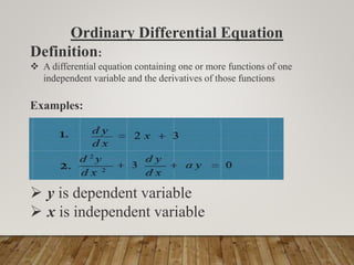
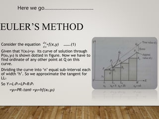
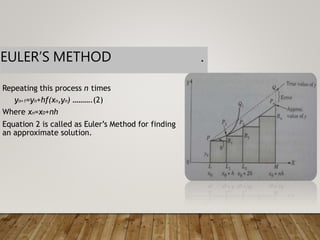
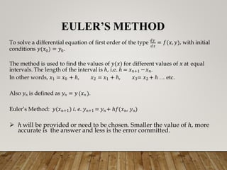
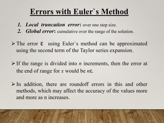
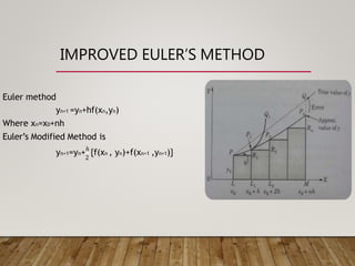
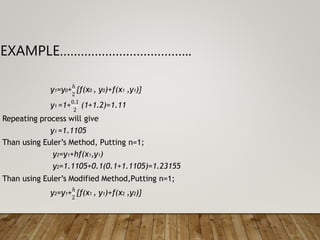
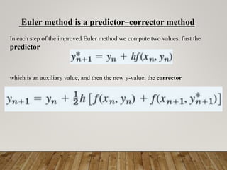
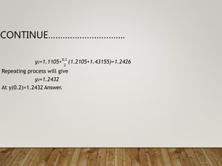
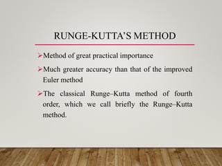
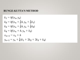
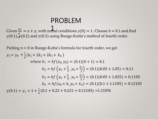
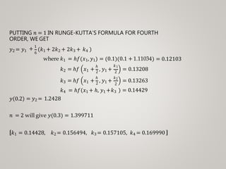
This document summarizes and compares several numerical methods for solving ordinary differential equations (ODEs): - Euler's method approximates the tangent line at each step to find successive y-values. While simple, it has local truncation errors that accumulate. - Improved Euler's method takes the average slope between the current and next steps to give a more accurate approximation. - Runge-Kutta methods such as the fourth-order method provide much greater accuracy than Euler or improved Euler by using multiple slope estimates within each step. 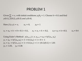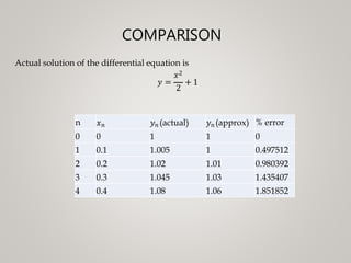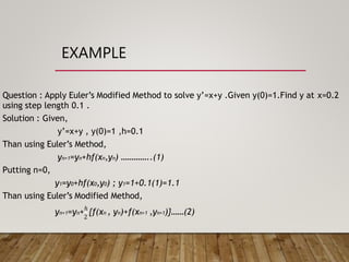An example applies each method to the ODE dy/dx = x + y to compare their results in solving for successive y-values out to x = 0.3.

1. Topic:
Numerical method for ODEs
Euler Method
Improved Euler Method
Runge-kutta’s Method
Prepared by:
Sohaib Siddique Butt
University of Gujrat
NUMERICALANALYSIS

2. Ordinary Differential Equation
Definition:
 A differential equation containing one or more functions of one
independent variable and the derivatives of those functions
Examples:
 y is dependent variable
 x is independent variable

3. Solution to Ordinary Differential
Equations
Analytical solutions: Eigenvalues, time
constants, damping coefficients
Numerical solutions: Euler Method, Runge-
Kutta Method

4. EULER’S METHOD
𝑑𝑥
Consider the equation 𝑑𝑦
=f(x,y) …….(1)
Given that Y(x0)=y0 its curve of solution through
P(x0,y0) is shown dotted in figure. Now we have to
find ordinate of any other point at Q on this
curve.
Dividing the curve into ‘n’ equal sub-interval each
of width ‘h’. So we approximate the tangent for
LL1
So Y1=L1P1=LP+R1P1
=y0+PR1 tan𝜃 =y0+hf(x0,y0)
Here we go………………………………..

5. EULER’S METHOD .
Repeating this process n times
yn+1=yn+hf(xn,yn) ……….(2)
Where xn=x0+nh
Equation 2 is called as Euler’s Method for finding
an approximate solution.

6. EULER’S METHOD
𝑑𝑥
To solve a differential equation of first order of the type 𝑑𝑦
= 𝑓 𝑥, 𝑦 , with initial
0 0conditions 𝑦 𝑥 = 𝑦 .
The method is used to find the values of 𝑦(𝑥) for different values of 𝑥 at equal
intervals. The length of the interval is ℎ, i.e. ℎ = 𝑥 𝑛+1 −𝑥 𝑛.
In other words, 𝑥1 = 𝑥0 + ℎ, 𝑥2 = 𝑥1 + ℎ, 𝑥3= 𝑥2 + ℎ … etc.
Also 𝑦 𝑛 is defined as 𝑦 𝑛 = 𝑦 𝑥 𝑛 .
Euler’s Method: 𝑦 𝑥 𝑛+1 𝑖. 𝑒. 𝑦 𝑛+1 = 𝑦 𝑛 + ℎ𝑓(𝑥 𝑛, 𝑦 𝑛)
 ℎ will be provided or need to be chosen. Smaller the value of ℎ, more
accurate is the answer and less is the error committed.

7. PROBLEM 1
Given 𝑑𝑦
= 𝑥, with initial conditions 𝑦 0 = 1. Choose ℎ = 0.1 and find
𝑑𝑥
𝑦 0.1 , 𝑦 0.2 , 𝑦 0.3 and 𝑦 0.4 .
Here 𝑓 𝑥, 𝑦 = 𝑥, 𝑥0 = 0, 𝑦0 = 1
𝑥1 = 𝑥0 + ℎ = 0 + 0.1 = 0.1, 𝑥2 = 𝑥1 + ℎ = 0.2, 𝑥3= 𝑥2 + ℎ =0.3, 𝑥4 = 0.4
Using Euler’s Method: 𝑦 𝑥 𝑛+1 𝑖. 𝑒. 𝑦 𝑛+1 = 𝑦 𝑛 + ℎ𝑓(𝑥 𝑛, 𝑦 𝑛)
𝑦1 = 𝑦0 + ℎ𝑓 𝑥0, 𝑦0
𝑦2 = 𝑦1 + ℎ𝑓 𝑥1, 𝑦1
= 1 + 0.1 𝑥0
= 1 + 0.1 𝑥1
= 1 + 0 = 1
= 1 + (0.1)(0.1) = 1.01
𝑦3 = 1.03, 𝑦4 =1.06

8. Errors with Euler`s Method
1. Local truncation error: over one step size.
2. Global error: cumulative over the range of the solution.
The error ε using Euler`s method can be approximated
using the second term of the Taylor series expansion.
If the range is divided into n increments, then the error at
the end of range for x would be nε.
In addition, there are roundoff errors in this and other
methods, which may affect the accuracy of the values more
and more as n increases.

9. COMPARISON
Actual solution of the differential equation is
𝑥2
2
𝑦 = + 1
n 𝑥 𝑛 𝑦 𝑛 (actual) 𝑦 𝑛 (approx) % error
0 0 1 1 0
1 0.1 1.005 1 0.497512
2 0.2 1.02 1.01 0.980392
3 0.3 1.045 1.03 1.435407
4 0.4 1.08 1.06 1.851852

10. IMPROVED EULER’S METHOD
In the Euler’s improved method , The curve of the solution in the interval LL1 is
approximates by the tangent at P such as at P1 we have,
Y1=y0+hf(x0,y0)
Than the slope of the curve of the solution through P1 is computed at the tangent at P1
to P1Q1 is drawn meeting the ordinate through L2 in P2(x0+2h,y2)……1
Now we find better approximation y1’ of y(x0+h) by taking the slope of the curve as the
mean of the slope of the tangent at P and P1 i.e.
Y1’=y0+ ℎ
{f(x0+y0)+f(X0+h,Y1)}…..2
2
As the slope of the tangent at P1 is not known, We take Y1 is found in equation (1)

11. IMPROVED EULER’S METHOD
Euler method
yn+1 =yn+hf(xn,yn)
Where xn=x0+nh
Euler’s Modified Method is
2
yn+1=yn+ℎ
{f(xn , yn)+f(xn+1 ,yn+1)}

12. Euler method is a predictor–corrector method
In each step of the improved Euler method we compute two values, first the
predictor
which is an auxiliary value, and then the new y-value, the corrector

13. EXAMPLE
Question : Apply Euler’s Modified Method to solve y’=x+y .Given y(0)=1.Find y at x=0.2
using step length 0.1 .
Solution : Given,
y’=x+y , y(0)=1 ,h=0.1
Than using Euler’s Method,
yn+1=yn+hf(xn,yn) …………..(1)
Putting n=0,
y1=y0+hf(x0,y0) ; y1=1+0.1(1)=1.1
Than using Euler’s Modified Method,
2
yn+1=yn+ℎ
{f(xn , yn)+f(xn+1 ,yn+1)}……(2)

14. EXAMPLE………………………………..
2
y1=y0+ℎ
{f(x0 , y0)+f(x1 ,y1)}
y1 =1+0.1
(1+1.2)=1.11
2
Repeating process will give
y1 =1.1105
Than using Euler’s Method, Putting n=1;
y2=y1+hf(x1,y1)
y2=1.1105+0.1(0.1+1.1105)=1.23155
Than using Euler’s Modified Method,Putting n=1;
2
y2=y1+ℎ
{f(x1 , y1)+f(x2 ,y2)}

15. CONTINUE…………………………..
y2=1.1105+0.1
(1.2105+1.43155)=1.2426
2
Repeating process will give
y2=1.2432
At y(0.2)=1.2432 Answer.

16. RUNGE-KUTTA’S METHOD
Method of great practical importance
Much greater accuracy than that of the improved
Euler method
The classical Runge–Kutta method of fourth
order, which we call briefly the Runge–Kutta
method.

17. RUNGE-KUTTA’S METHOD

18. PROBLEM
1
𝑑
𝑥
Given 𝑑𝑦
= 𝑥 + 𝑦, with initial conditions 𝑦 0 = 1. Choose ℎ = 0.1 and find
𝑦 0.1 , 𝑦 0.2 and 𝑦 0.3 using Runge-Kutta’s method of fourth order.
Putting 𝑛 = 0 in Runge-Kutta’s formula for fourth order, we get
𝑦1 = 𝑦0 + 1
6
𝑘1 + 2𝑘2 + 2𝑘3 + 𝑘4
where 𝑘1 = ℎ𝑓 𝑥0, 𝑦0 = 0.1 0 + 1 = 0.1
ℎ
= 0.1 0.05 + 1.05 = 0.11𝑘2 = ℎ𝑓
𝑘3 = ℎ𝑓
ℎ
𝑥0 + 2
, 𝑦0 +
𝑥0 + 2
, 𝑦0 +
𝑘1
2
𝑘2
2
𝑘4 = ℎ𝑓 𝑥0 + ℎ, 𝑦0 + 𝑘3
= 0.1 0.05 + 1.055
= 0.1 0.1 + 1.1105
= 0.1105
= 0.12105
1𝑦 0.1 = 𝑦 = 1 + 1
6
0.1 + 0.22 + 0.221 + 0.12105 =1.11034

19. PUTTING 𝑛 = 1 IN RUNGE-KUTTA’S FORMULA FOR FOURTH
ORDER, WE GET
𝑦2 = 𝑦1 + 1
6
𝑘1 + 2𝑘2 + 2𝑘3 + 𝑘4
where 𝑘1 = ℎ𝑓 𝑥1, 𝑦1 = = 0.12103
ℎ
0.1 0.1 + 1.11034
= 0.13208𝑘2 = ℎ𝑓
𝑘3 = ℎ𝑓
ℎ
𝑥1 + 2
, 𝑦1 +
𝑥1 + 2
, 𝑦1 +
𝑘1
2
𝑘2
2
= 0.13263
= 0.14429
𝑦 0.2
𝑘4 = ℎ𝑓 𝑥1 + ℎ, 𝑦1 +𝑘3
= 𝑦2 = 1.2428
𝑛 = 2 will give 𝑦 0.3 = 1.399711
𝑘1 = 0.14428, 𝑘2 = 0.156494, 𝑘3 = 0.157105, 𝑘4 = 0.169990