Engineering Dynamic Ch II -kinematics of a particle.pptx
1.
Addis Ababa University
AddisAbaba Institute of Technology
School of Mechanical & Industrial Engineering
Engineering Mechanics II (Dynamics)
MEng 2052
Chapter Two
Kinematics of Particles
2.
Kinematics: is thebranch of dynamics which describes the
motion of bodies without reference to the forces that either
causes the motion or are generated as a result of the motion.
Kinematics is often referred to as the “geometry of motion”
AAiT School of Mechanical and Industrial Engineering - SMiE 2
Introduction
3.
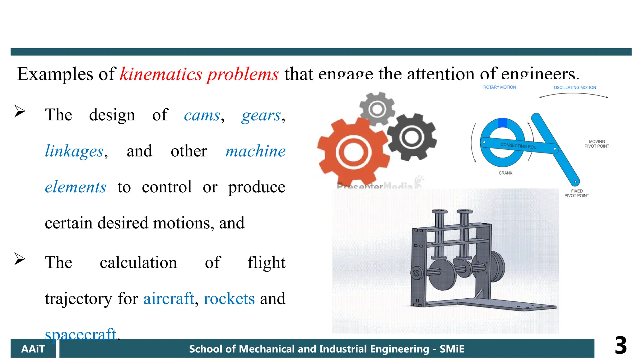
Examples of kinematicsproblems that engage the attention of engineers.
AAiT School of Mechanical and Industrial Engineering - SMiE 3
The design of cams, gears,
linkages, and other machine
elements to control or produce
certain desired motions, and
The calculation of flight
trajectory for aircraft, rockets and
spacecraft.
4.
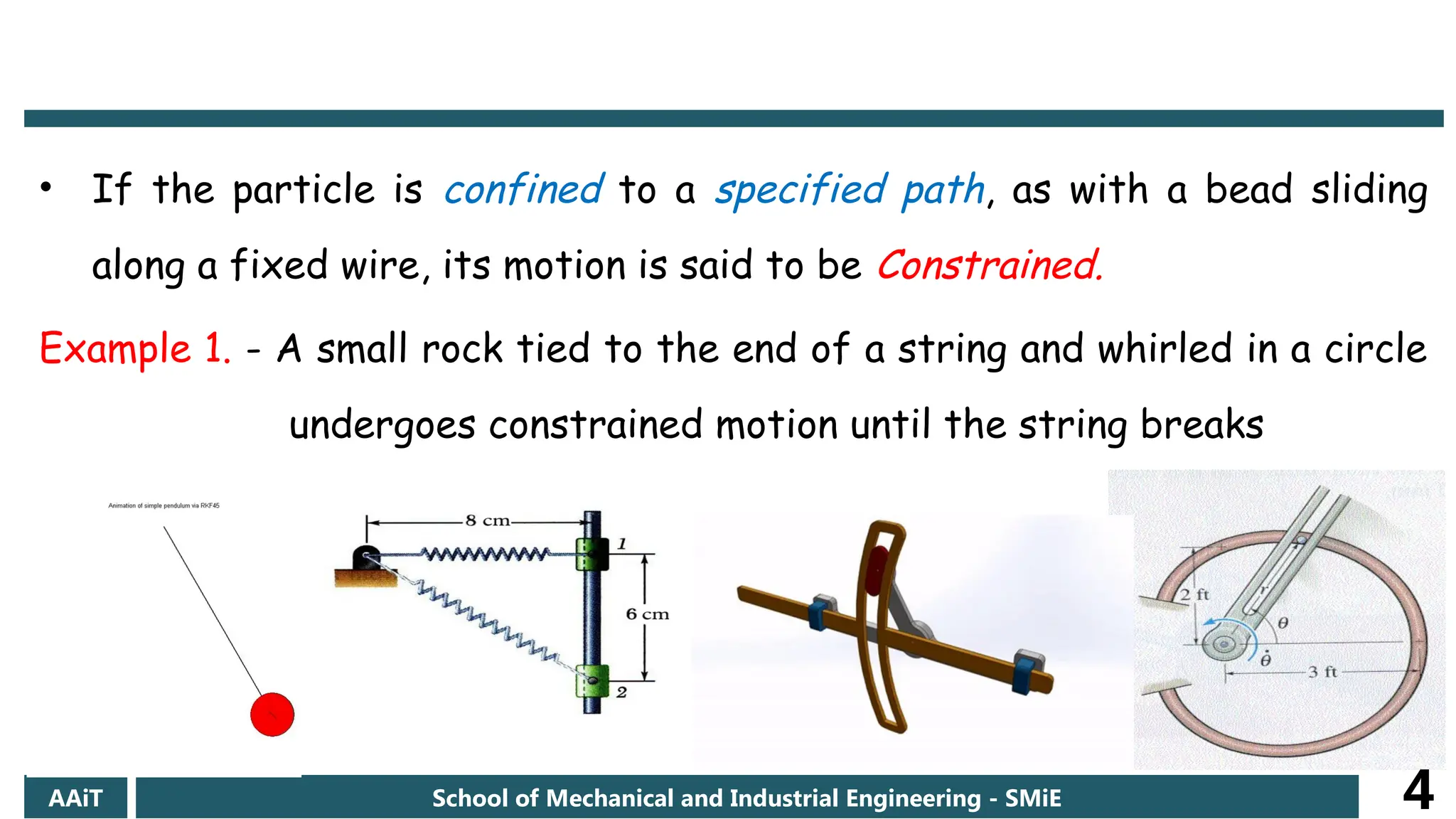
• If theparticle is confined to a specified path, as with a bead sliding
along a fixed wire, its motion is said to be Constrained.
Example 1. - A small rock tied to the end of a string and whirled in a circle
undergoes constrained motion until the string breaks
AAiT School of Mechanical and Industrial Engineering - SMiE 4
5.
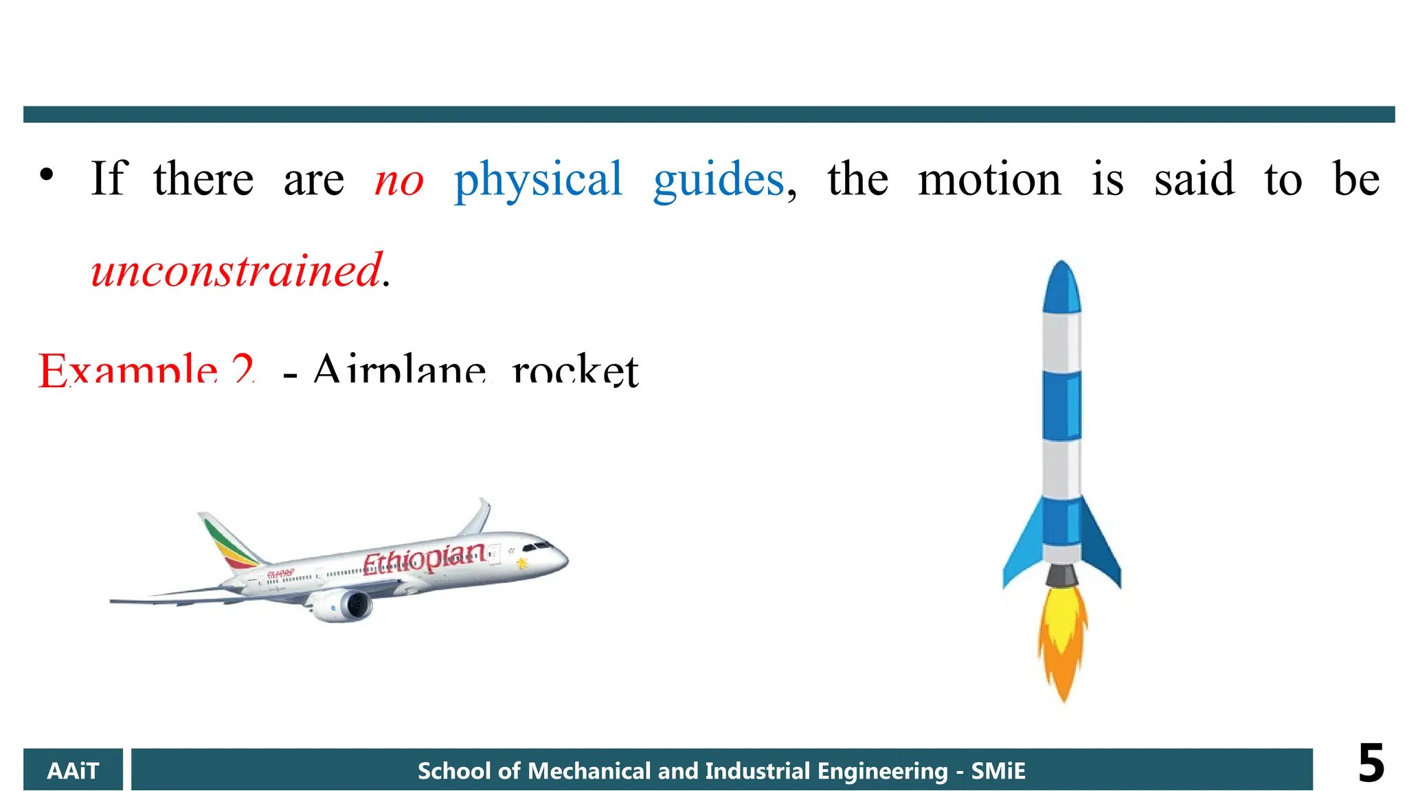
• If thereare no physical guides, the motion is said to be
unconstrained.
Example 2. - Airplane, rocket
AAiT School of Mechanical and Industrial Engineering - SMiE 5
6.
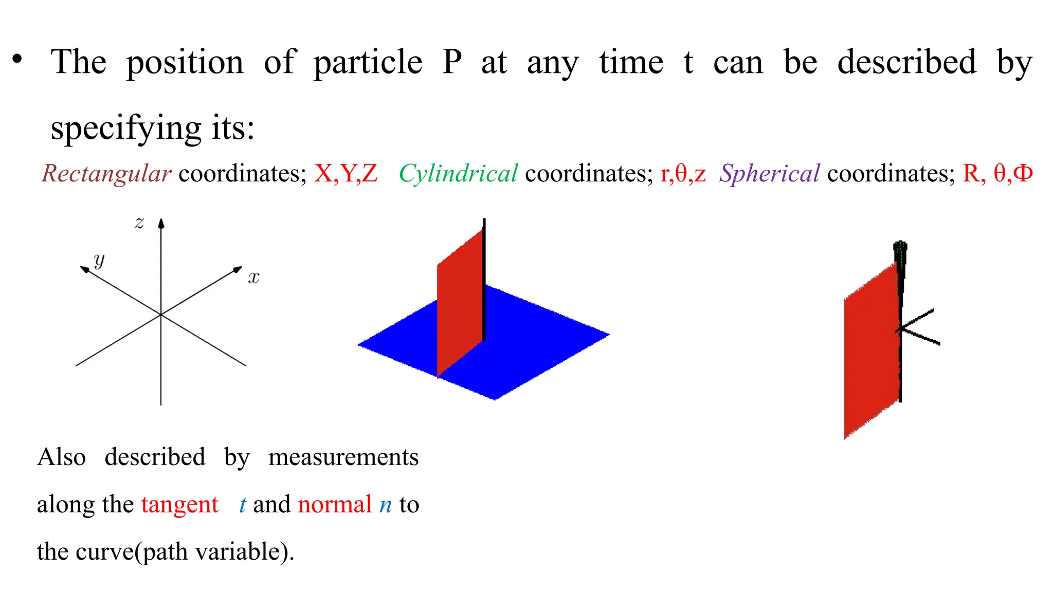
• The positionof particle P at any time t can be described by
specifying its:
Rectangular coordinates; X,Y,Z Cylindrical coordinates; r,θ,z Spherical coordinates; R, θ,Ф
Also described by measurements
along the tangent t and normal n to
the curve(path variable).
7.
• The motionof particles(or rigid bodies) may be described by
using coordinates measured from fixed reference axis
(absolute motion analysis) or by using coordinates measured
from moving reference axis (relative motion analysis).
AAiT School of Mechanical and Industrial Engineering - SMiE 7
8.
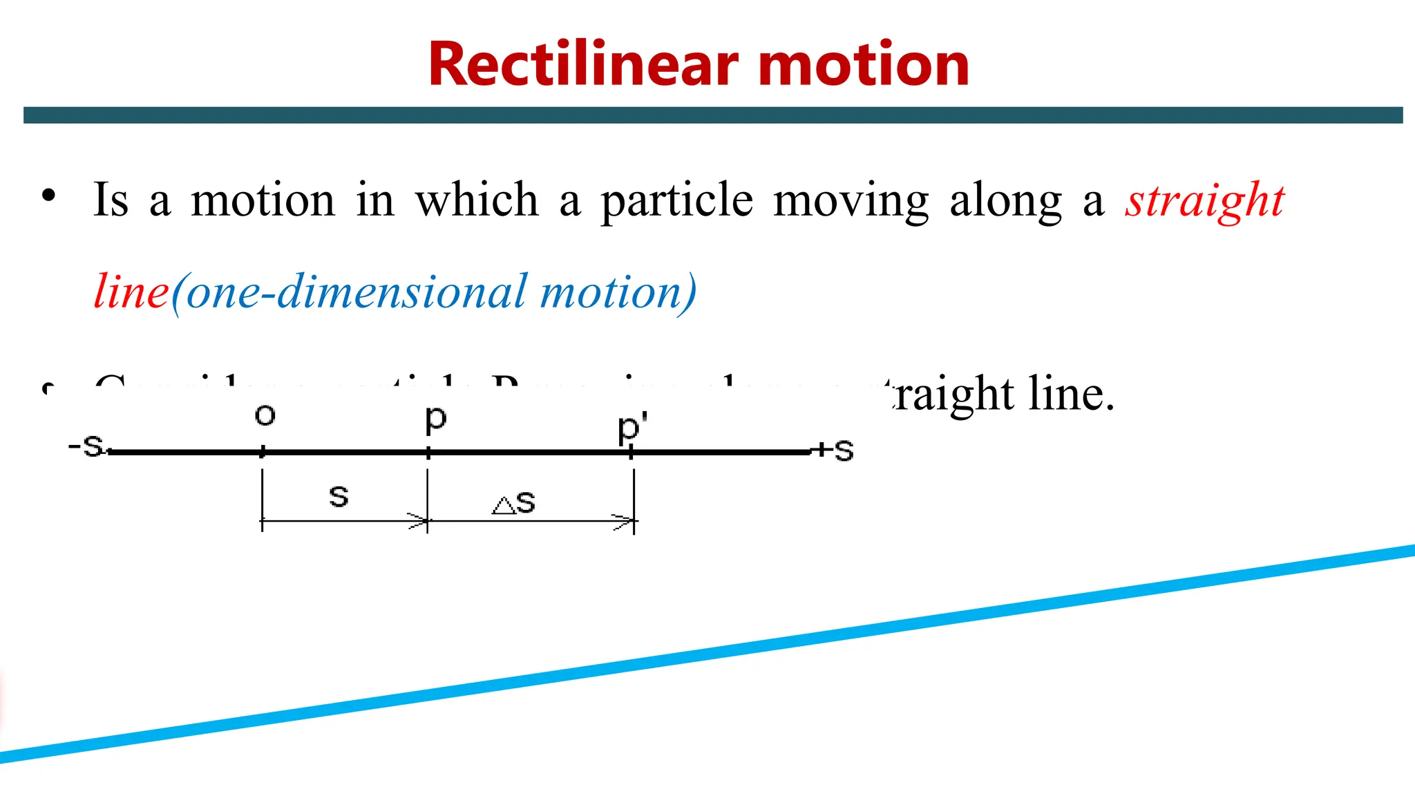
• Is amotion in which a particle moving along a straight
line(one-dimensional motion)
• Consider a particle P moving along a straight line.
Rectilinear motion
9.
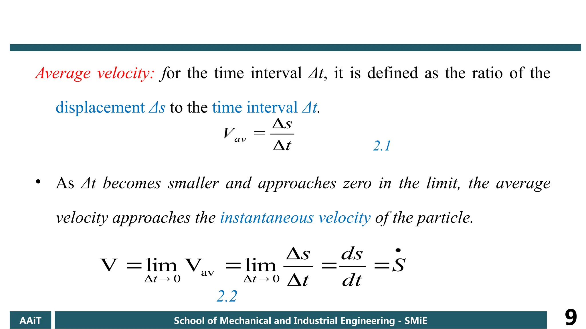
Average velocity: forthe time interval Δt, it is defined as the ratio of the
displacement Δs to the time interval Δt.
2.1
• As Δt becomes smaller and approaches zero in the limit, the average
velocity approaches the instantaneous velocity of the particle.
2.2
t
s
=
Vav
S
dt
ds
t
s
t
t 0
av
0
lim
V
lim
V
AAiT School of Mechanical and Industrial Engineering - SMiE 9
10.
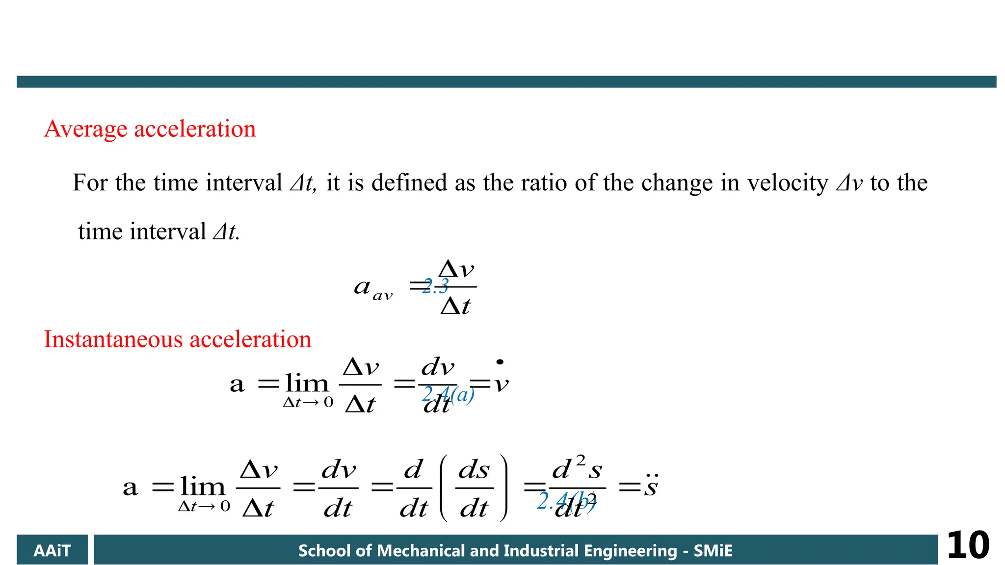
Average acceleration
For thetime interval Δt, it is defined as the ratio of the change in velocity Δv to the
time interval Δt.
2.3
Instantaneous acceleration
2.4(a)
2.4(b)
t
v
aav
v
dt
dv
t
v
t 0
lim
a
s
dt
s
d
dt
ds
dt
d
dt
dv
t
v
t
2
2
0
lim
a
AAiT School of Mechanical and Industrial Engineering - SMiE 10
11.
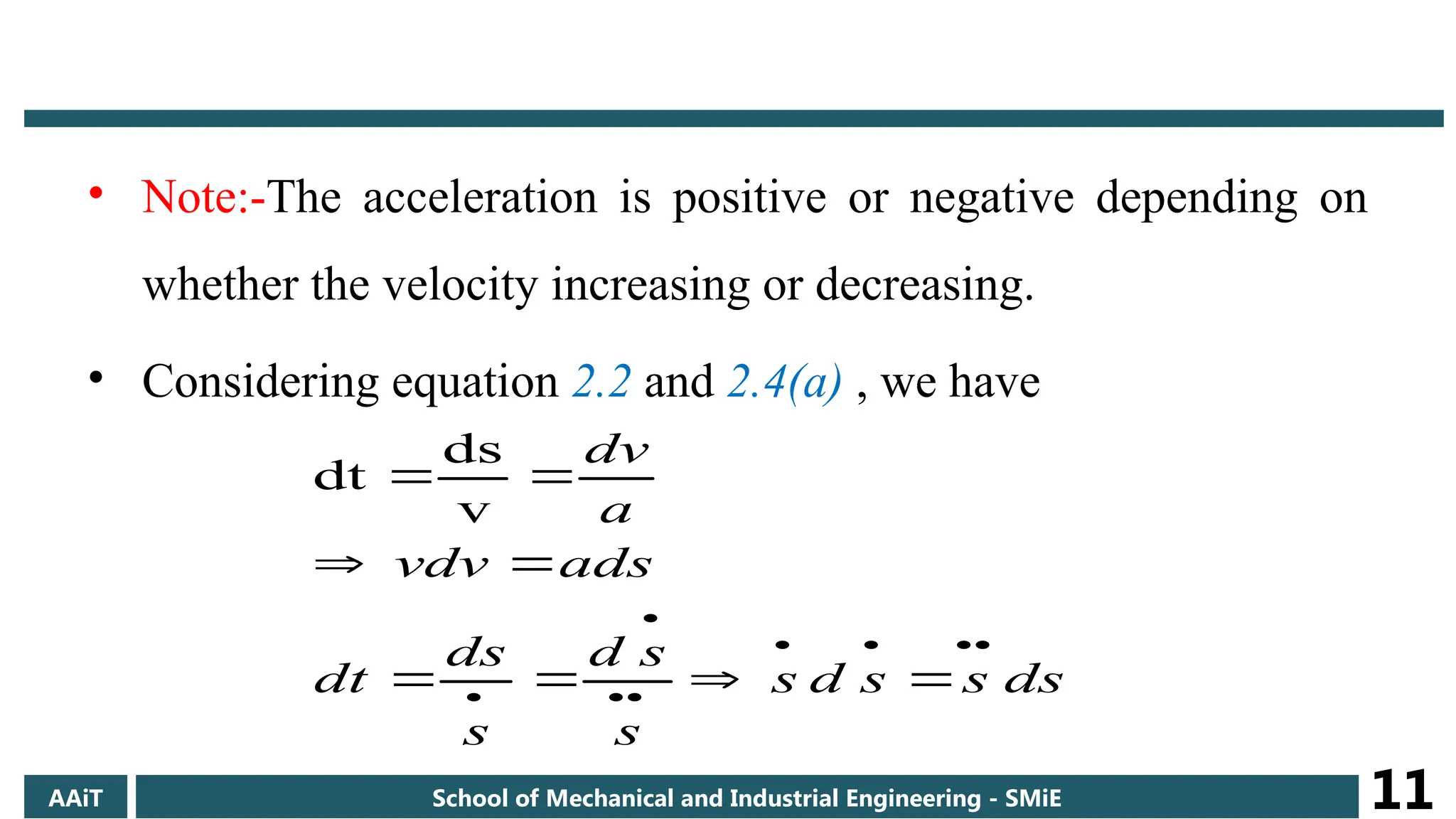
• Note:-The accelerationis positive or negative depending on
whether the velocity increasing or decreasing.
• Considering equation 2.2 and 2.4(a) , we have
ds
s
s
d
s
s
s
d
s
ds
dt
ads
vdv
a
dv
v
ds
dt
AAiT School of Mechanical and Industrial Engineering - SMiE 11
12.
AAiT School ofMechanical and Industrial Engineering - SMiE 12
General Representation of
Relationship among s, v, a & t.
13.
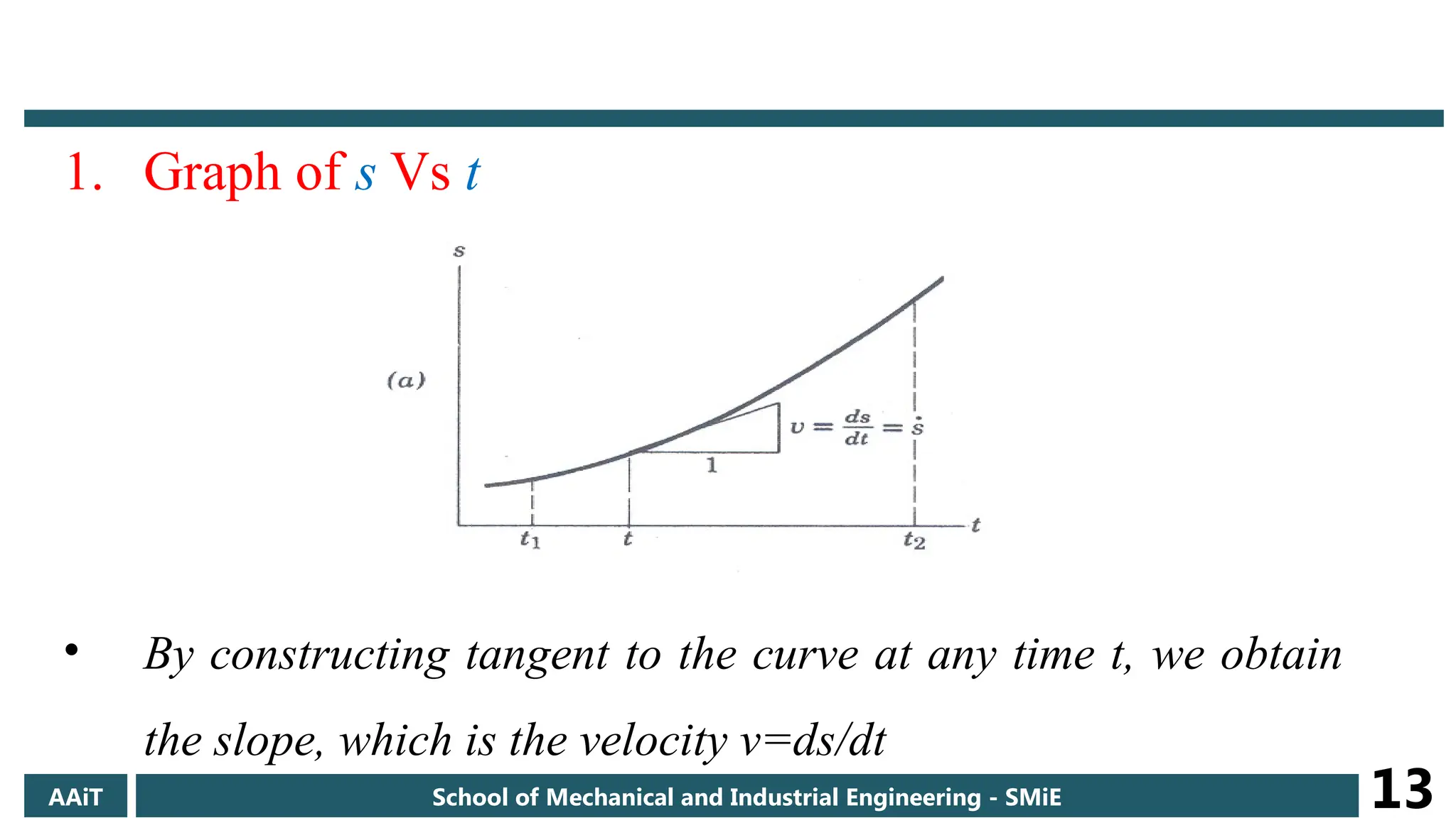
1. Graph ofs Vs t
• By constructing tangent to the curve at any time t, we obtain
the slope, which is the velocity v=ds/dt
AAiT School of Mechanical and Industrial Engineering - SMiE 13
14.
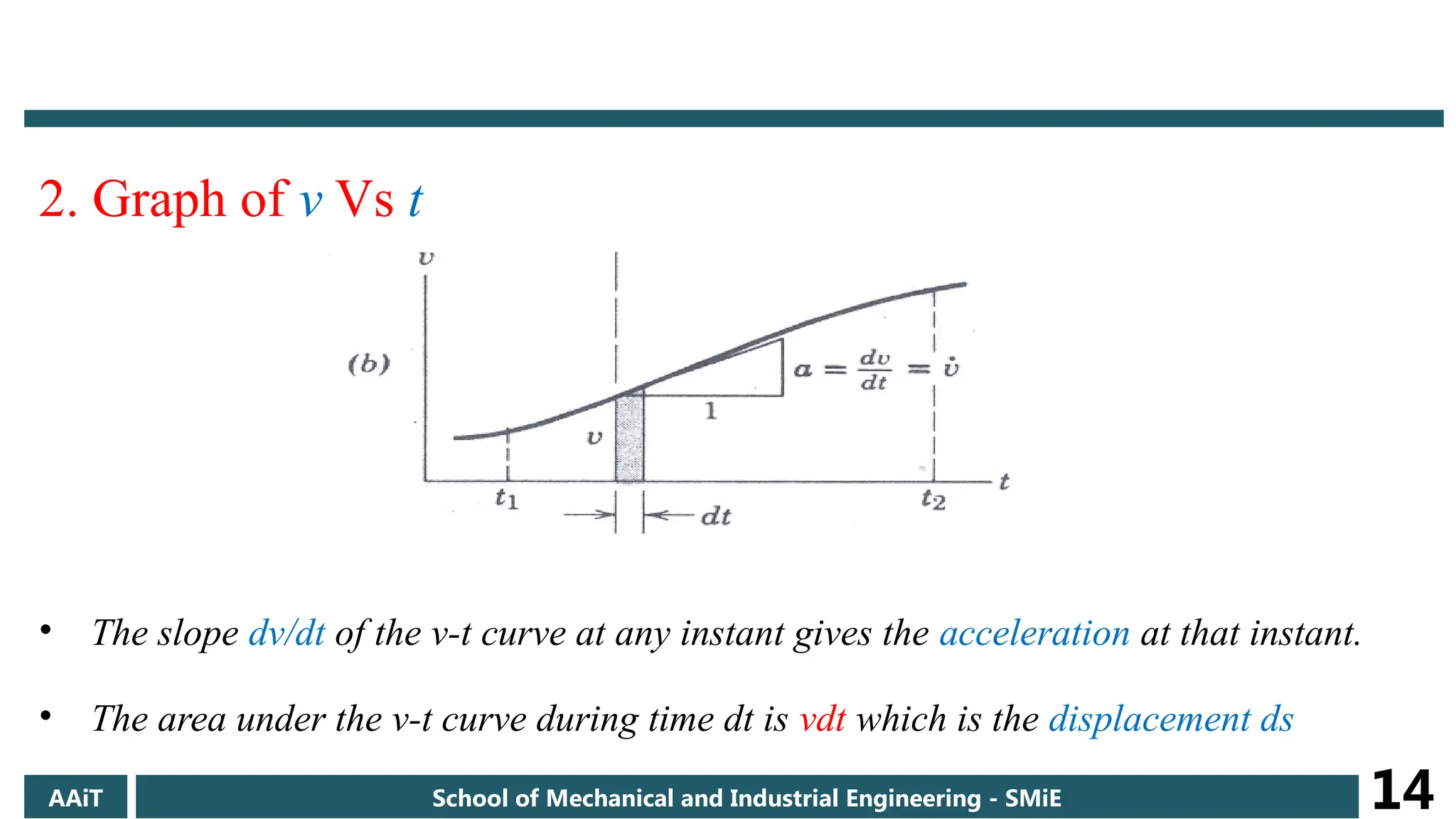
2. Graph ofv Vs t
• The slope dv/dt of the v-t curve at any instant gives the acceleration at that instant.
• The area under the v-t curve during time dt is vdt which is the displacement ds
AAiT School of Mechanical and Industrial Engineering - SMiE 14
15.
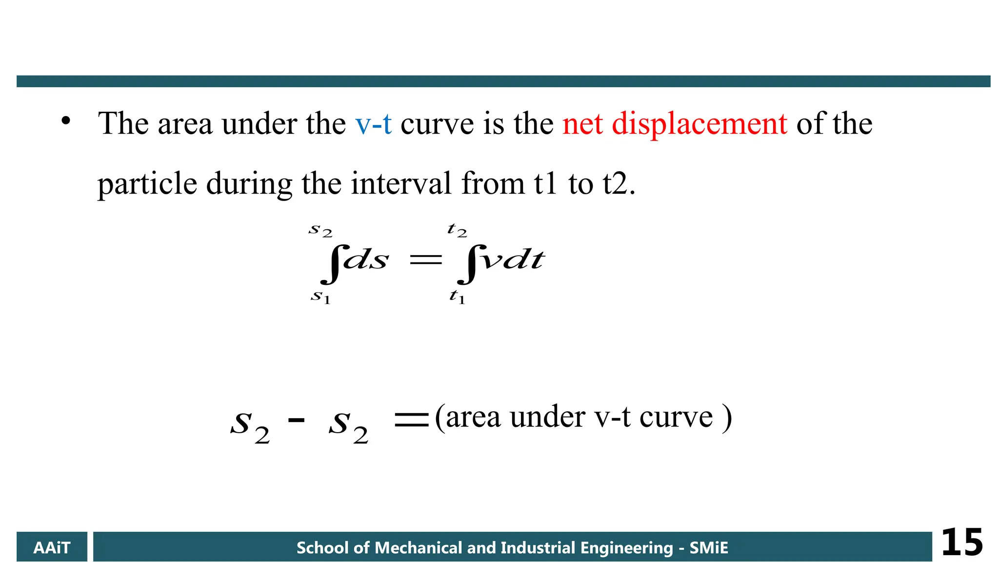
• The areaunder the v-t curve is the net displacement of the
particle during the interval from t1 to t2.
(area under v-t curve )
2
1
2
1
s
s
t
t
vdt
ds
2
2 s
s
AAiT School of Mechanical and Industrial Engineering - SMiE 15
16.
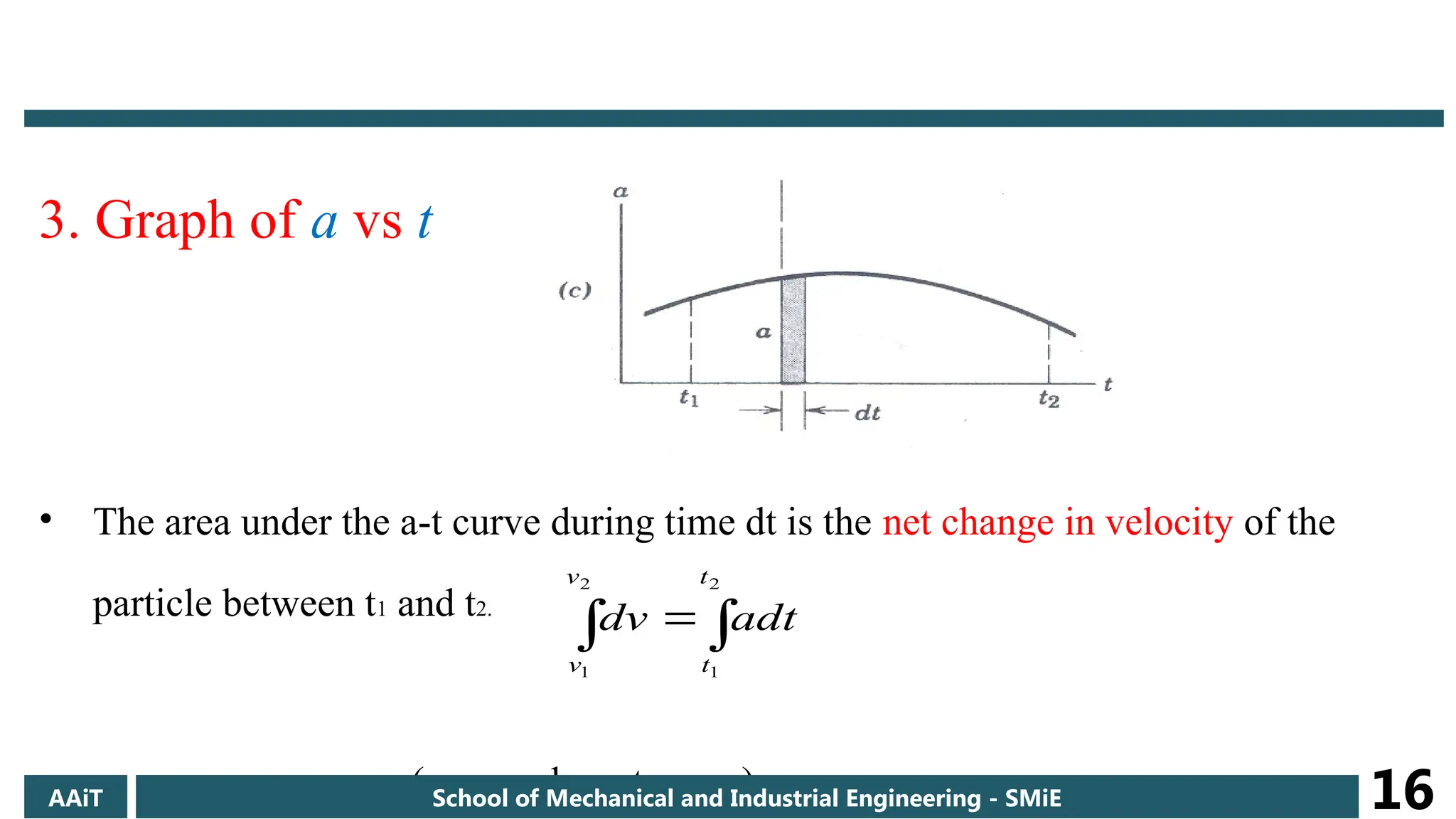
3. Graph ofa vs t
• The area under the a-t curve during time dt is the net change in velocity of the
particle between t1 and t2.
v2 - v1=(area under a-t curve)
2
1
2
1
v
v
t
t
adt
dv
AAiT School of Mechanical and Industrial Engineering - SMiE 16
17.
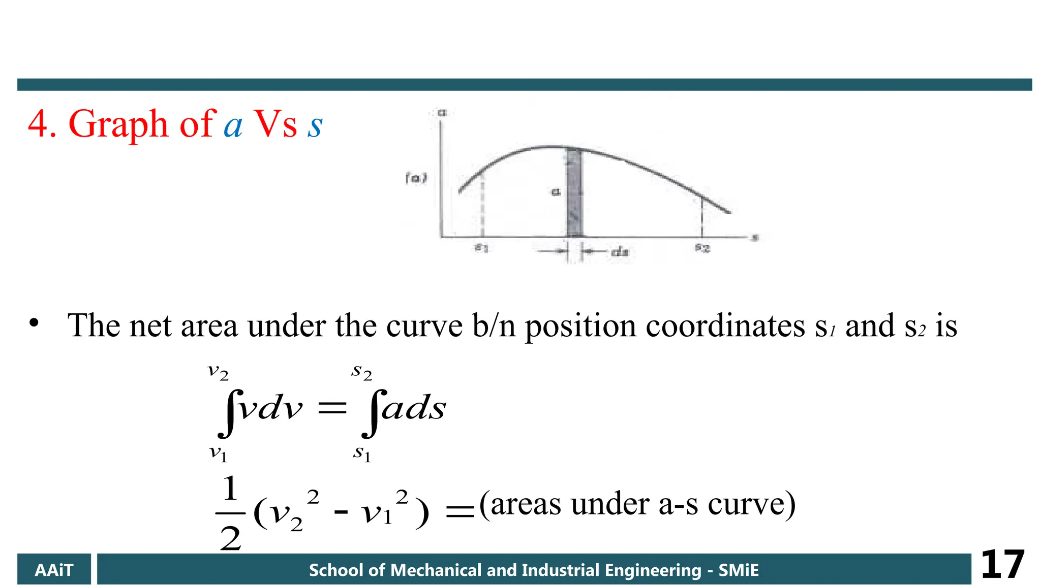
4. Graph ofa Vs s
• The net area under the curve b/n position coordinates s1 and s2 is
(areas under a-s curve)
2
1
2
1
v
v
s
s
ads
vdv
)
(
2
1 2
1
2
2 v
v
AAiT School of Mechanical and Industrial Engineering - SMiE 17
18.
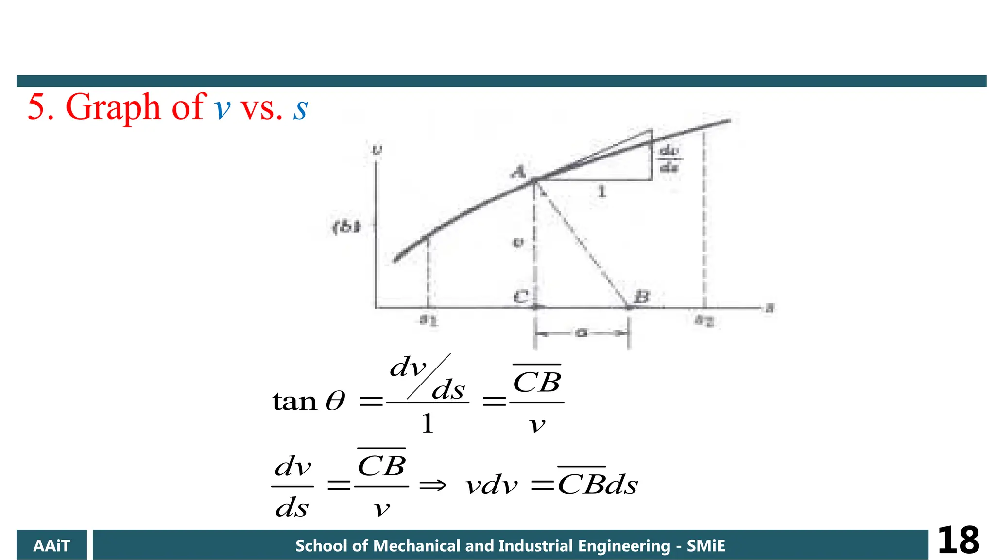
5. Graph ofv vs. s
ds
CB
vdv
v
CB
ds
dv
v
CB
ds
dv
1
tan
AAiT School of Mechanical and Industrial Engineering - SMiE 18
19.
• The graphicalrepresentations described are useful for:-
visualizing the relationships among the several motion quantities.
approximating results by graphical integration or differentiation when a lack
of knowledge of the mathematical relationship prevents its expression as an
explicit mathematical function .
experimental data and motions that involve discontinuous relationship b/n
variables.
AAiT School of Mechanical and Industrial Engineering - SMiE 19
20.
AAiT School ofMechanical and Industrial Engineering - SMiE 20
General Methods for Determining the
Velocity and Displacement Functions
Representation of Relationship among s, v,
a & t.
21.
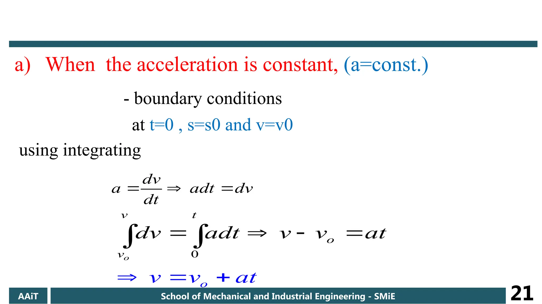
a) When theacceleration is constant, (a=const.)
- boundary conditions
at t=0 , s=s0 and v=v0
using integrating
dv
adt
dt
dv
a
0
o
o
v t
o
v
v v at
dv adt v v at
AAiT School of Mechanical and Industrial Engineering - SMiE 21
22.
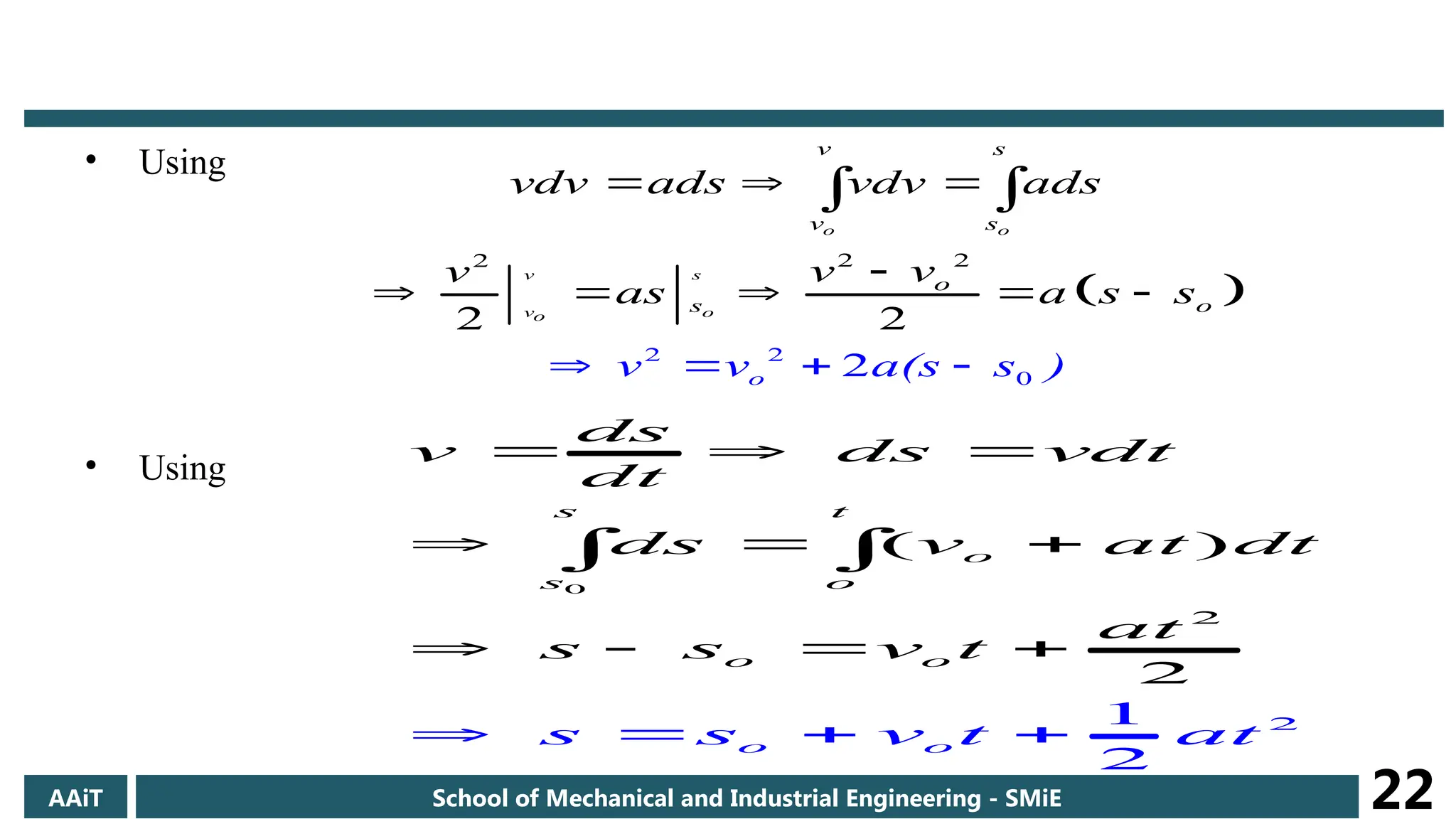
• Using
• Using
2
2
0
2
2
2
2
2 2
o o
v s
v o
o
v s
v s
o
s
o
o
v v a(s s )
vdv ads vdv ads
v v
v
as a s s
0
2
2
1
2
2
( )
s t
o
s
o
o o
o
o
ds
v ds vdt
dt
ds v at dt
at
s s
s s v t t
v t
a
AAiT School of Mechanical and Industrial Engineering - SMiE 22
23.
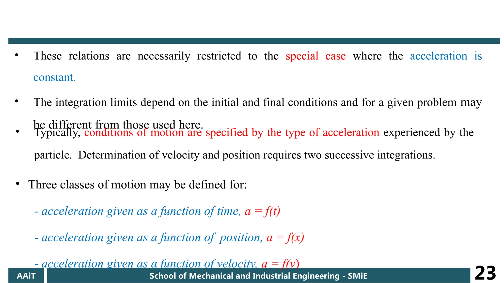
• These relationsare necessarily restricted to the special case where the acceleration is
constant.
• The integration limits depend on the initial and final conditions and for a given problem may
be different from those used here.
AAiT School of Mechanical and Industrial Engineering - SMiE 23
• Typically, conditions of motion are specified by the type of acceleration experienced by the
particle. Determination of velocity and position requires two successive integrations.
• Three classes of motion may be defined for:
- acceleration given as a function of time, a = f(t)
- acceleration given as a function of position, a = f(x)
- acceleration given as a function of velocity, a = f(v)
24.
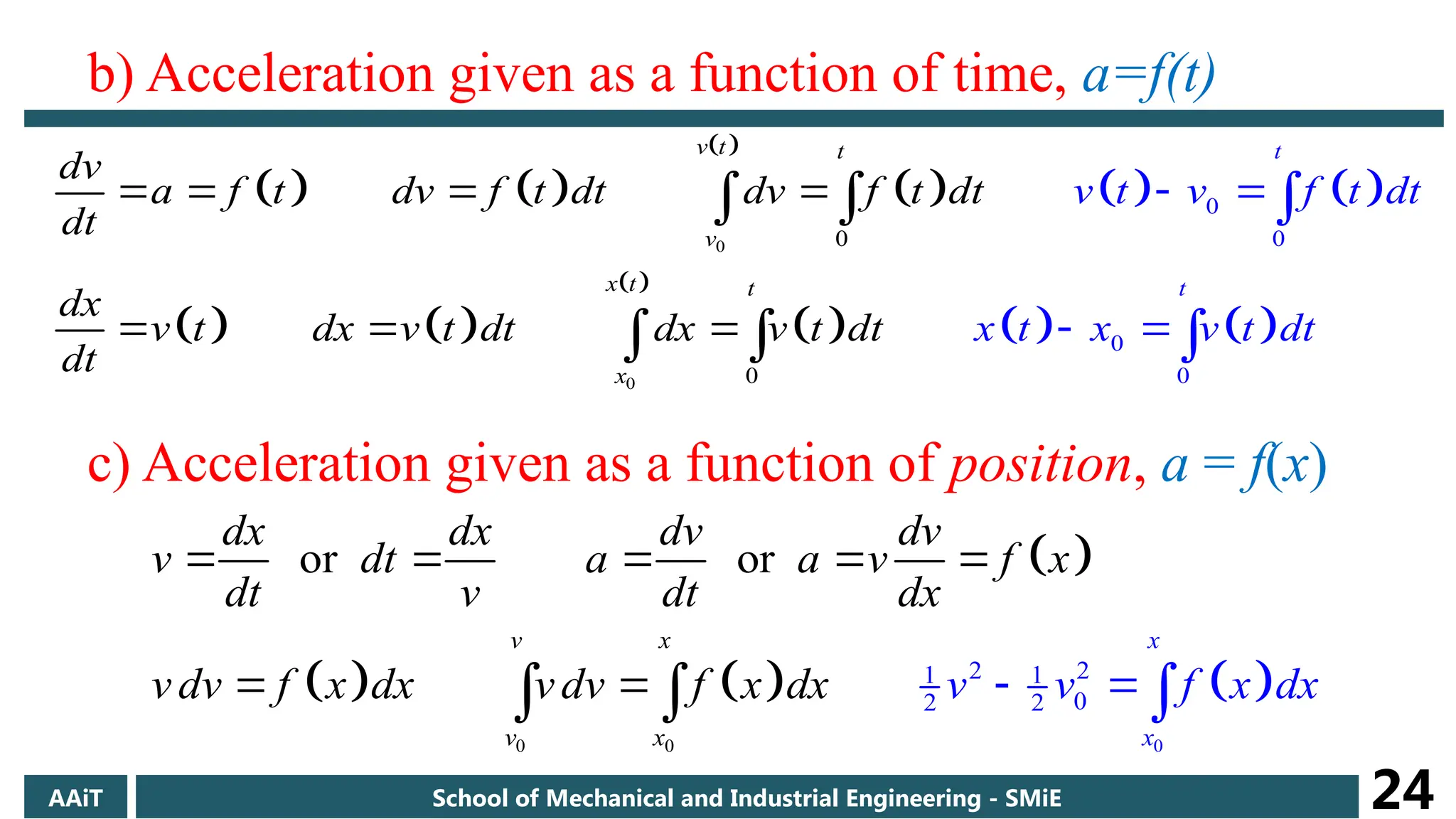
b) Acceleration givenas a function of time, a=f(t)
0
0
0
0
0
0
0
0
t
v t t
v
x t t
t
x
v t v f t dt
x t x v t
dv
a f t dv f t dt dv f t dt
t dt
dt
dx
v t dx v dt dx v t dt
dt
c) Acceleration given as a function of position, a = f(x)
0 0 0
2 2
1 1
0
2 2
or or
x
x
v x
v x
dx dx dv dv
v dt a a v f x
dt v dt dx
v d v
v f x dx v dv f x v f x
d d
x x
AAiT School of Mechanical and Industrial Engineering - SMiE 24
25.
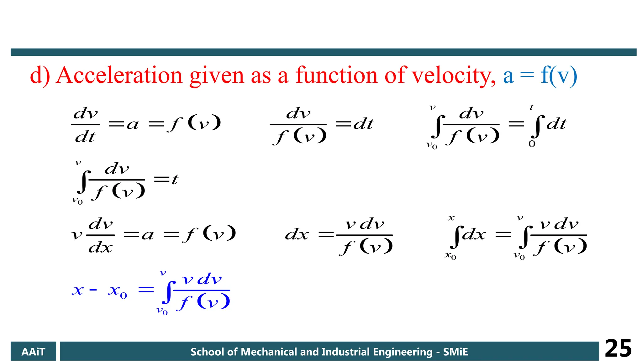
d) Acceleration givenas a function of velocity, a = f(v)
0
0
0 0
0
0
0
v t
v
x v
x
v
v
v
v
v
dv dv dv
a f v dt dt
dt f v f v
dv
t
f v
dv v dv v dv
v a f v dx dx
dx
x
f v
x
f
v dv
v
v
f
AAiT School of Mechanical and Industrial Engineering - SMiE 25
26.
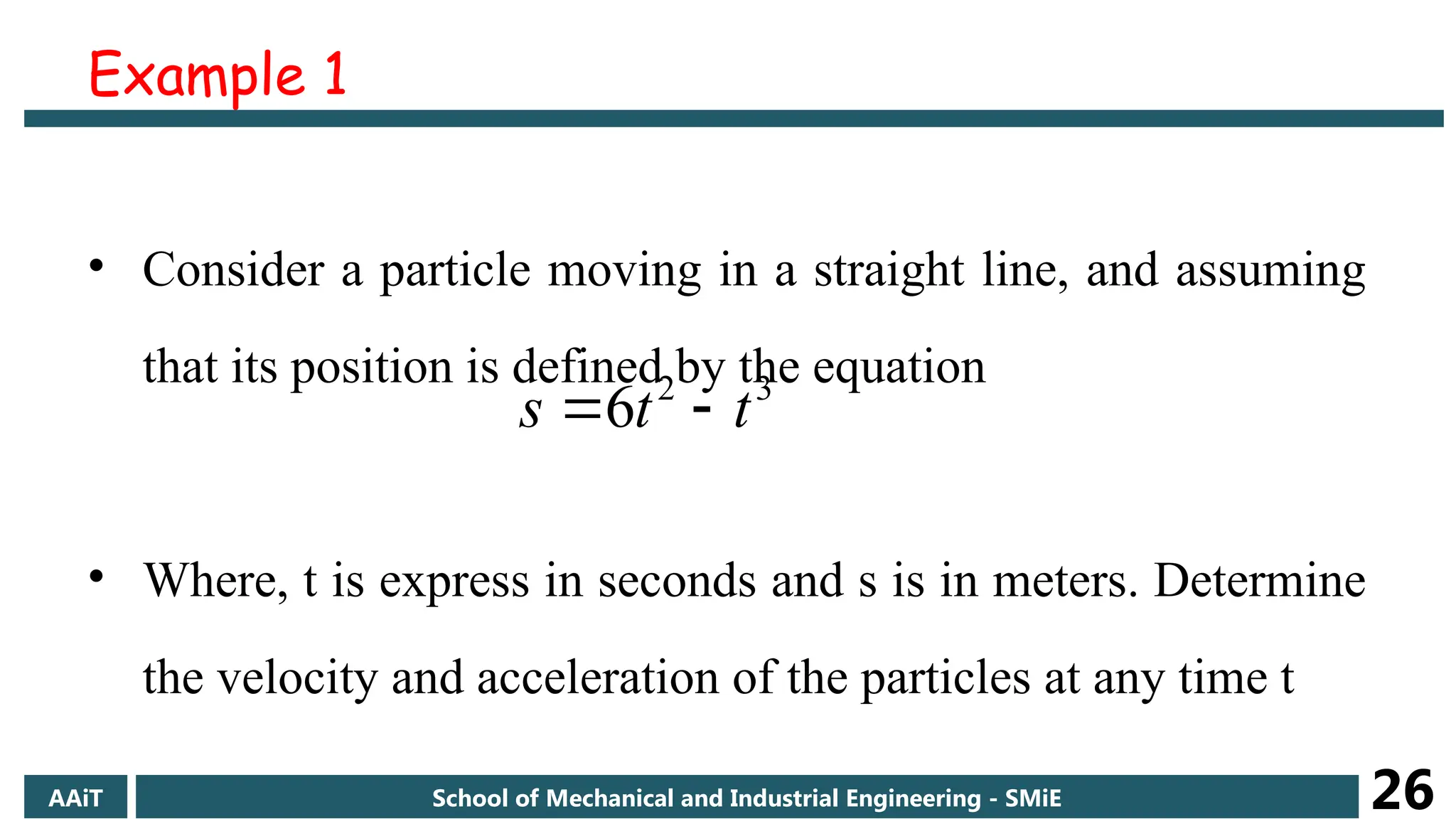
Example 1
• Considera particle moving in a straight line, and assuming
that its position is defined by the equation
• Where, t is express in seconds and s is in meters. Determine
the velocity and acceleration of the particles at any time t
3
2
6 t
t
s
AAiT School of Mechanical and Industrial Engineering - SMiE 26
27.
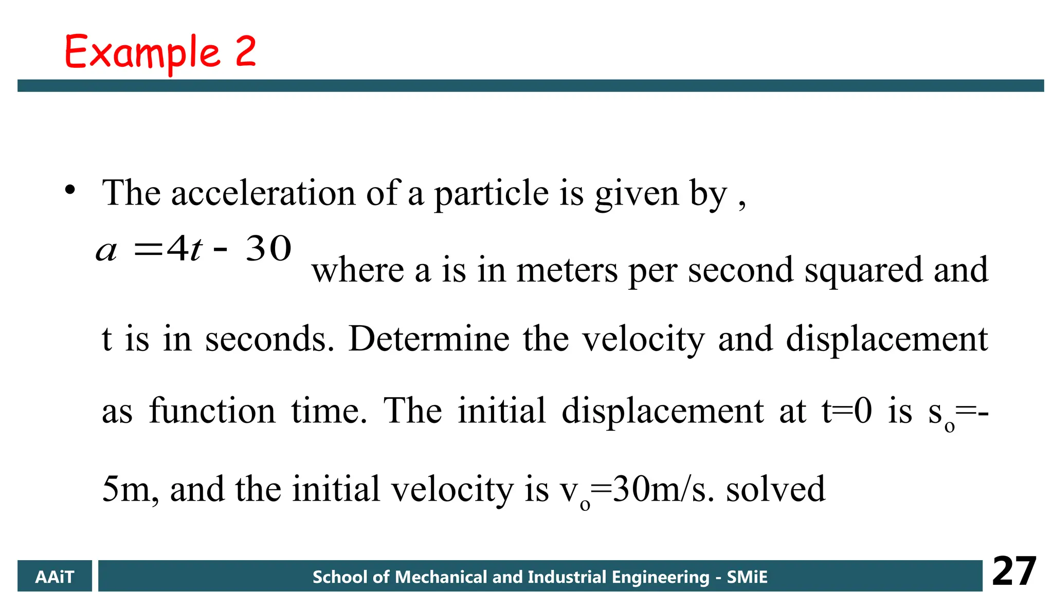
Example 2
• Theacceleration of a particle is given by ,
where a is in meters per second squared and
t is in seconds. Determine the velocity and displacement
as function time. The initial displacement at t=0 is so=-
5m, and the initial velocity is vo=30m/s. solved
30
4
t
a
AAiT School of Mechanical and Industrial Engineering - SMiE 27
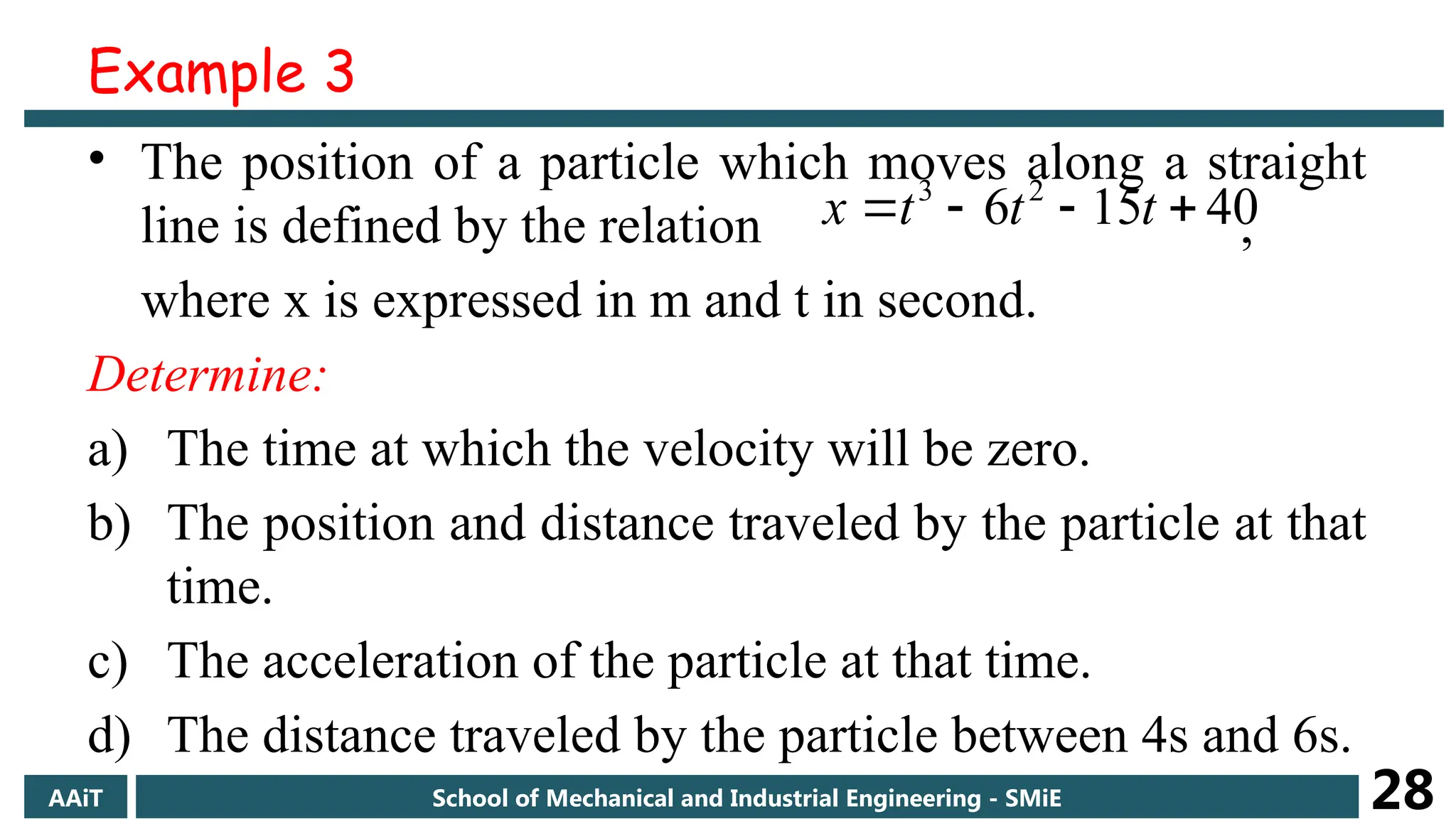
28.
• The positionof a particle which moves along a straight
line is defined by the relation ,
where x is expressed in m and t in second.
Determine:
a) The time at which the velocity will be zero.
b) The position and distance traveled by the particle at that
time.
c) The acceleration of the particle at that time.
d) The distance traveled by the particle between 4s and 6s.
40
15
6 2
3
t
t
t
x
AAiT School of Mechanical and Industrial Engineering - SMiE 28
Example 3
29.
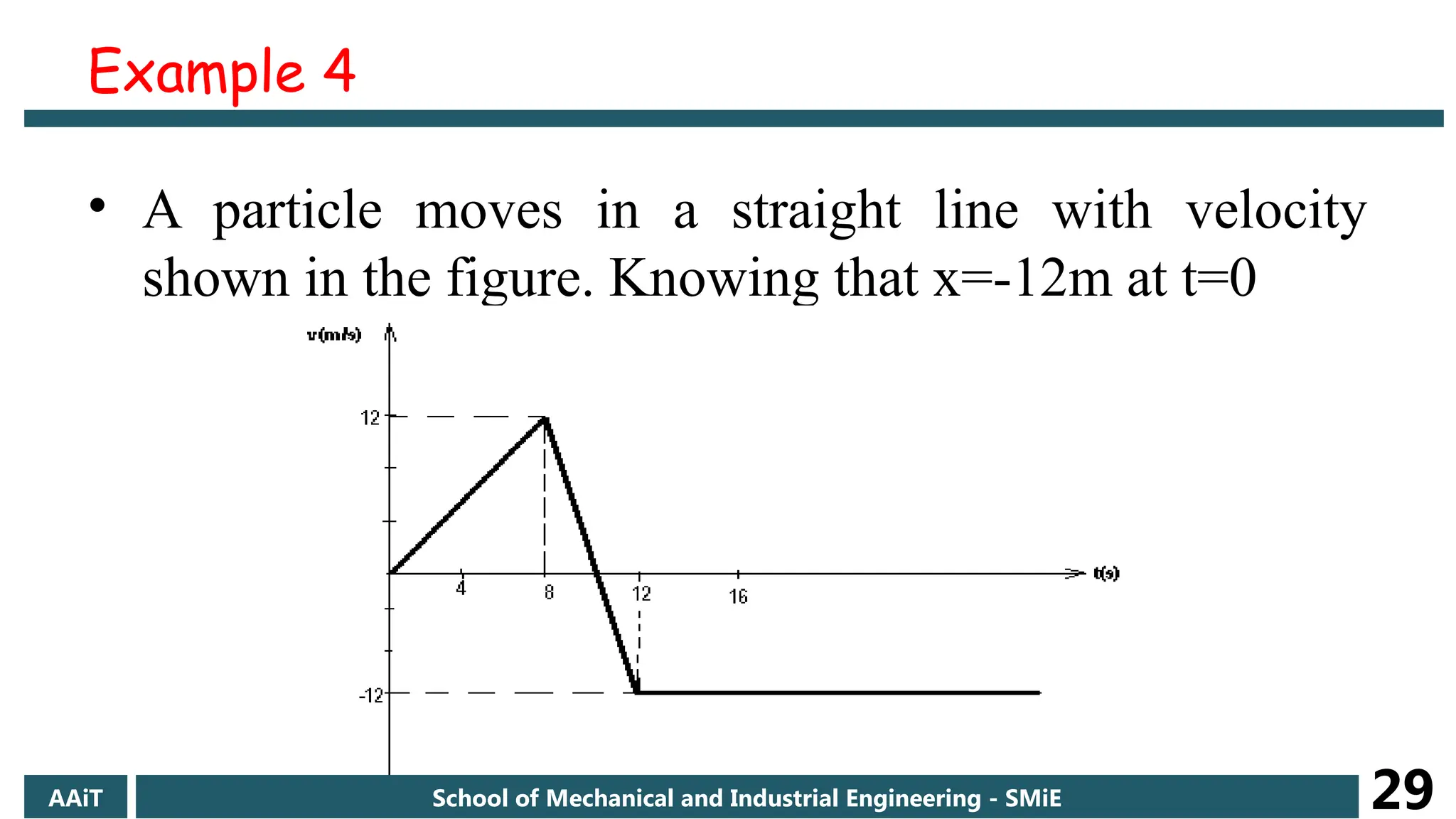
• A particlemoves in a straight line with velocity
shown in the figure. Knowing that x=-12m at t=0
AAiT School of Mechanical and Industrial Engineering - SMiE 29
Example 4
30.
• Draw thea-t and x-t graphs, and
• Determine:
a) The total distance traveled by the particle when t=12s.
b) The two values of t for which the particle passes the origin.
c) The max. value of the position coordinate of the particle.
d) The value of t for which the particle is at a distance of 15m
from the origin.
AAiT School of Mechanical and Industrial Engineering - SMiE 30
31.
AAiT School ofMechanical and Industrial Engineering - SMiE 31
Plane Curvilinear Motion
32.
Curvilinear Motion ofa Particle
• When a particle moves along a curve other than a straight line,
we say that the particle is in curvilinear motion
The analysis of motion of a particle along a curved path that lies
on a single plane.
AAiT School of Mechanical and Industrial Engineering - SMiE 32
33.
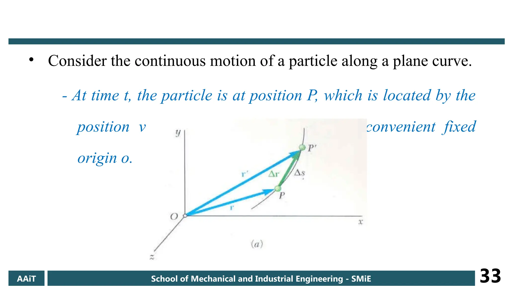
• Consider thecontinuous motion of a particle along a plane curve.
- At time t, the particle is at position P, which is located by the
position vector r measured from some convenient fixed
origin o.
AAiT School of Mechanical and Industrial Engineering - SMiE 33
34.
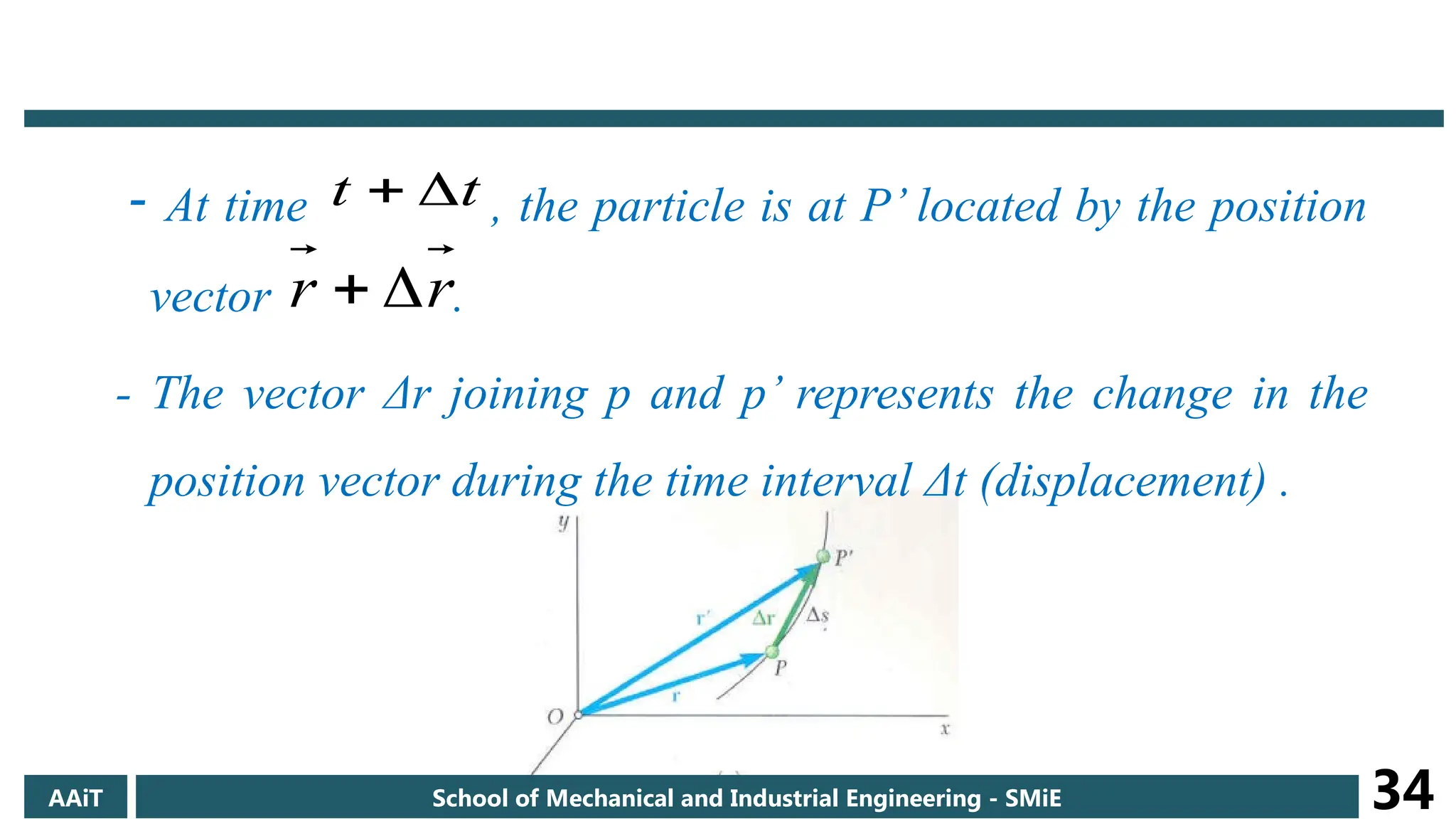
- At time, the particle is at P’ located by the position
vector .
- The vector Δr joining p and p’ represents the change in the
position vector during the time interval Δt (displacement) .
t
t
r
r
AAiT School of Mechanical and Industrial Engineering - SMiE 34
35.
• The distancetraveled by the particle as it moves along the
path from P to P’ is the scalar length Δs measured along the
path.
• The displacement of the particle, that represents the vector
change of position and is clearly independent of the choice
of origin.
AAiT School of Mechanical and Industrial Engineering - SMiE 35
36.
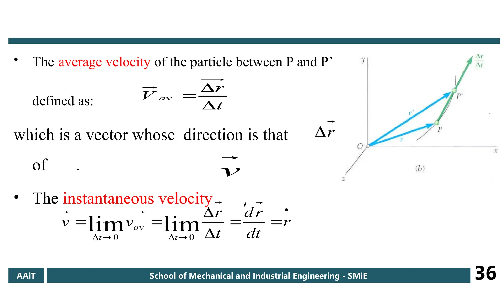
• The averagevelocity of the particle between P and P’
defined as:
which is a vector whose direction is that
of .
• The instantaneous velocity ,
t
r
V av
r
v
r
dt
r
d
t
r
v
v
t
av
t
lim
lim 0
0
AAiT School of Mechanical and Industrial Engineering - SMiE 36
37.
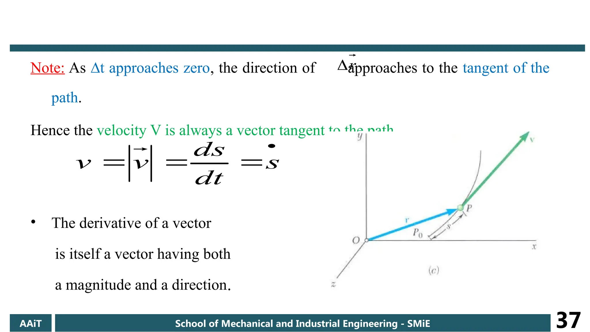
Note: As ∆tapproaches zero, the direction of approaches to the tangent of the
path.
Hence the velocity V is always a vector tangent to the path.
• The derivative of a vector
is itself a vector having both
a magnitude and a direction.
r
s
dt
ds
v
v
AAiT School of Mechanical and Industrial Engineering - SMiE 37
38.
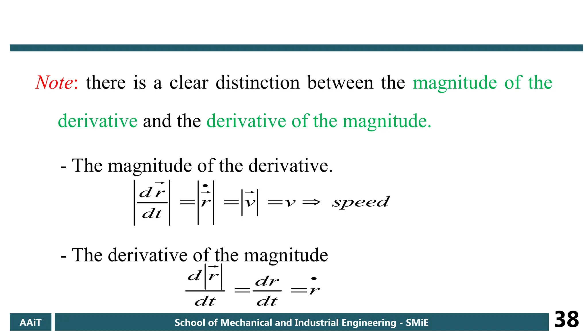
Note: there isa clear distinction between the magnitude of the
derivative and the derivative of the magnitude.
- The magnitude of the derivative.
- The derivative of the magnitude
speed
v
v
r
dt
r
d
r
dt
dr
dt
r
d
AAiT School of Mechanical and Industrial Engineering - SMiE 38
39.
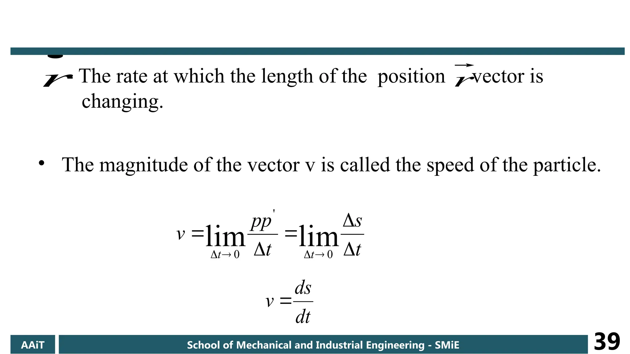
- The rateat which the length of the position vector is
changing.
• The magnitude of the vector v is called the speed of the particle.
t
s
t
pp
v
t
t
lim
lim 0
'
0
dt
ds
v
r r
AAiT School of Mechanical and Industrial Engineering - SMiE 39
40.
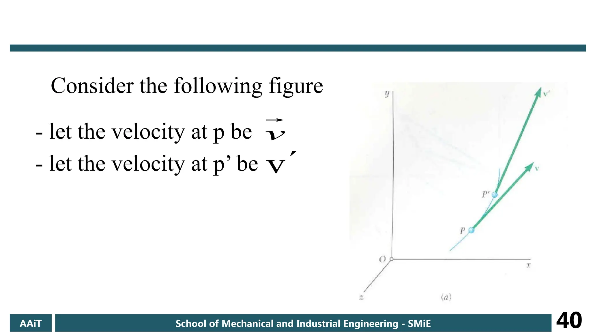
Consider the followingfigure
- let the velocity at p be
- let the velocity at p’ be
v
v
AAiT School of Mechanical and Industrial Engineering - SMiE 40
41.
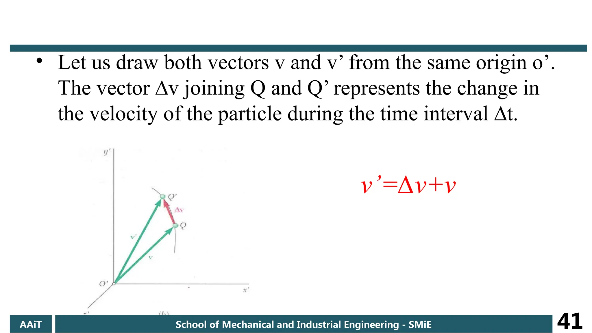
• Let usdraw both vectors v and v’ from the same origin o’.
The vector ∆v joining Q and Q’ represents the change in
the velocity of the particle during the time interval ∆t.
v’=∆v+v
AAiT School of Mechanical and Industrial Engineering - SMiE 41
42.
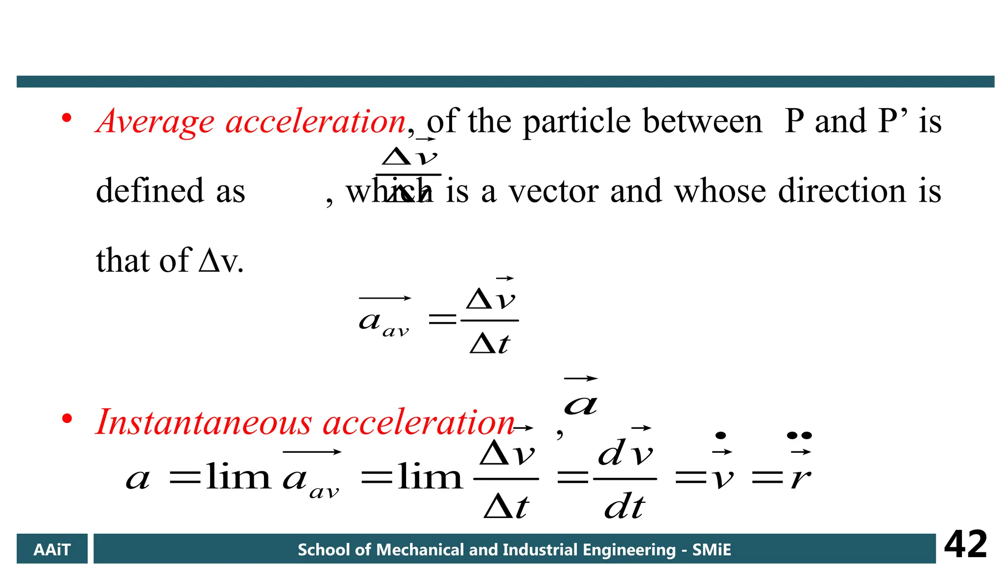
• Average acceleration,of the particle between P and P’ is
defined as , which is a vector and whose direction is
that of ∆v.
• Instantaneous acceleration ,
t
v
t
v
aav
a
r
v
dt
v
d
t
v
a
a av lim
lim
AAiT School of Mechanical and Industrial Engineering - SMiE 42
43.
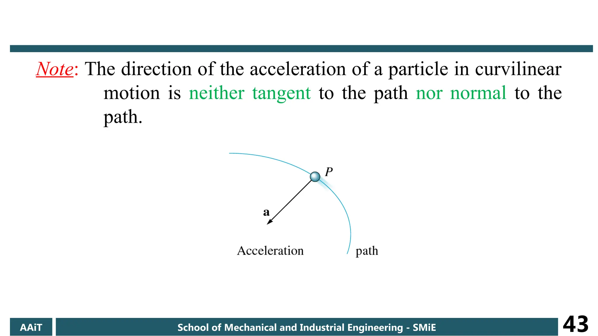
Note: The directionof the acceleration of a particle in curvilinear
motion is neither tangent to the path nor normal to the
path.
AAiT School of Mechanical and Industrial Engineering - SMiE 43
44.
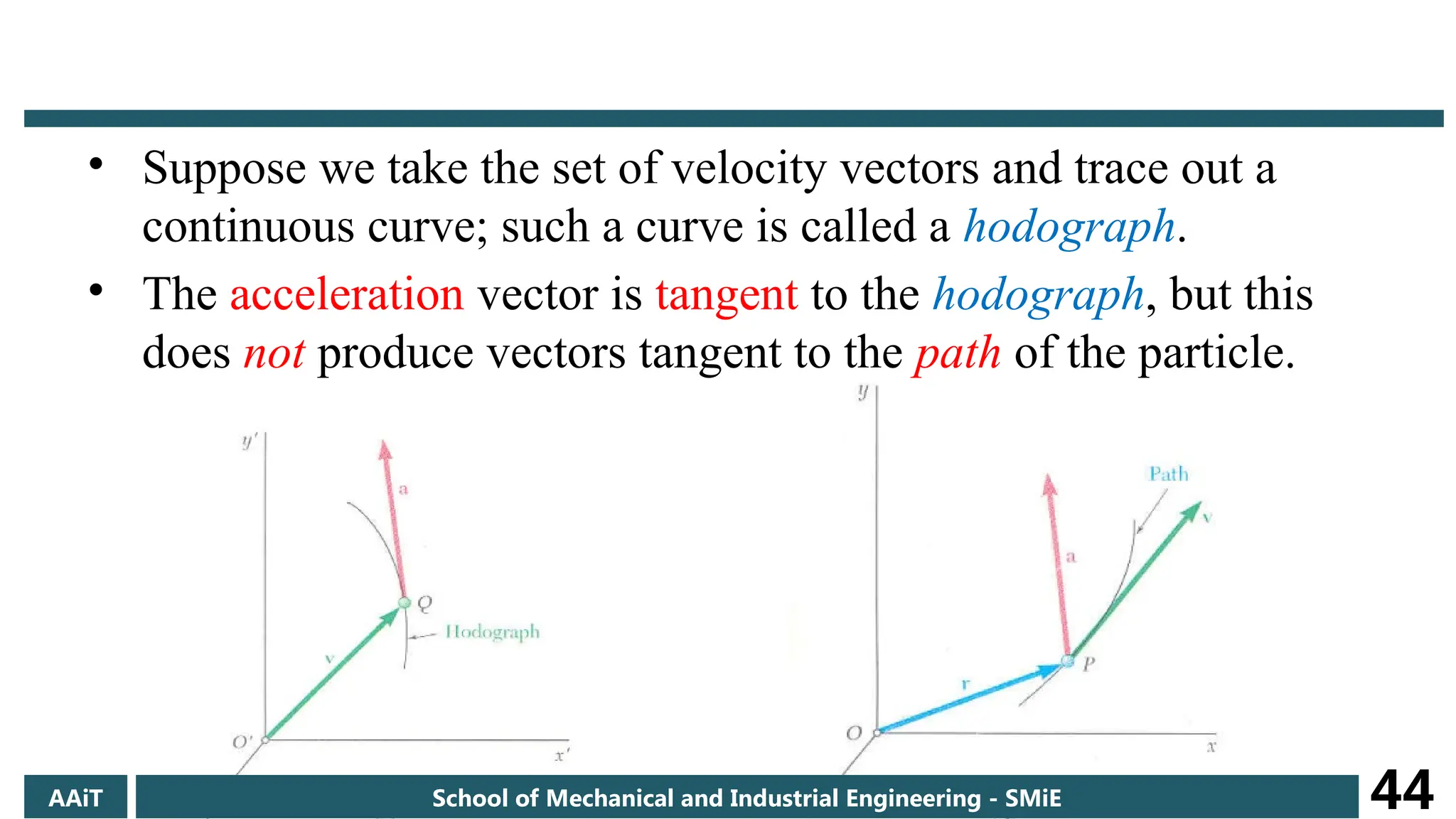
• Suppose wetake the set of velocity vectors and trace out a
continuous curve; such a curve is called a hodograph.
• The acceleration vector is tangent to the hodograph, but this
does not produce vectors tangent to the path of the particle.
AAiT School of Mechanical and Industrial Engineering - SMiE 44
45.
• This isparticularly useful for describing motions where the x,y and
z-components of acceleration are independently generated.
• When the position of a particle P is defined at any instant by its
rectangular coordinate x,y and z, it is convenient to resolve the
velocity v and the acceleration a of the particle into rectangular
components.
AAiT School of Mechanical and Industrial Engineering - SMiE 45
Rectangular co-ordinates (x-y-z)
46.
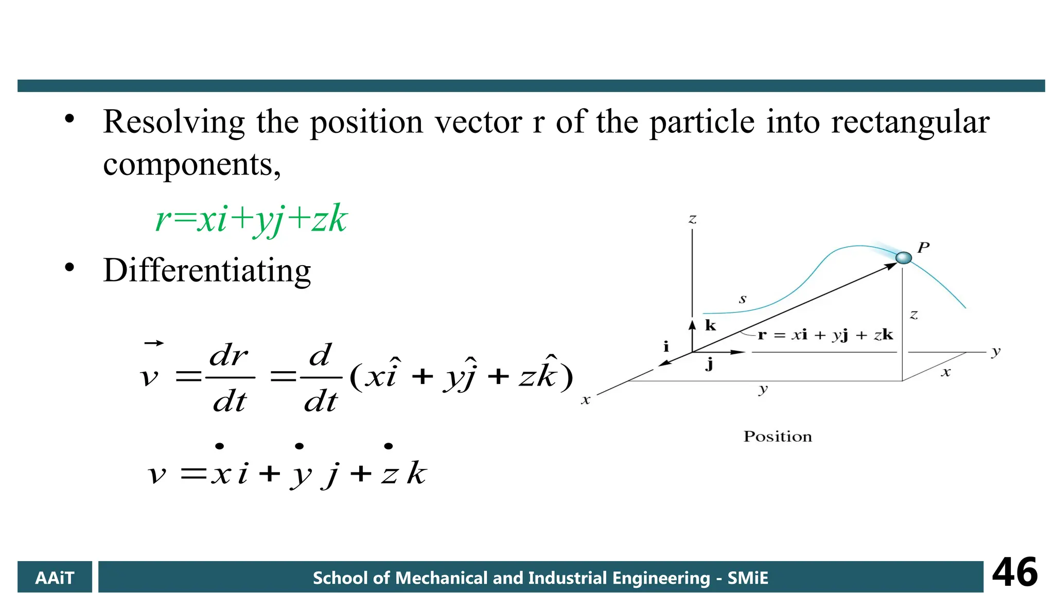
• Resolving theposition vector r of the particle into rectangular
components,
r=xi+yj+zk
• Differentiating
)
ˆ
ˆ
ˆ
( k
z
j
y
i
x
dt
d
dt
r
d
v
k
z
j
y
i
x
v
AAiT School of Mechanical and Industrial Engineering - SMiE 46
47.
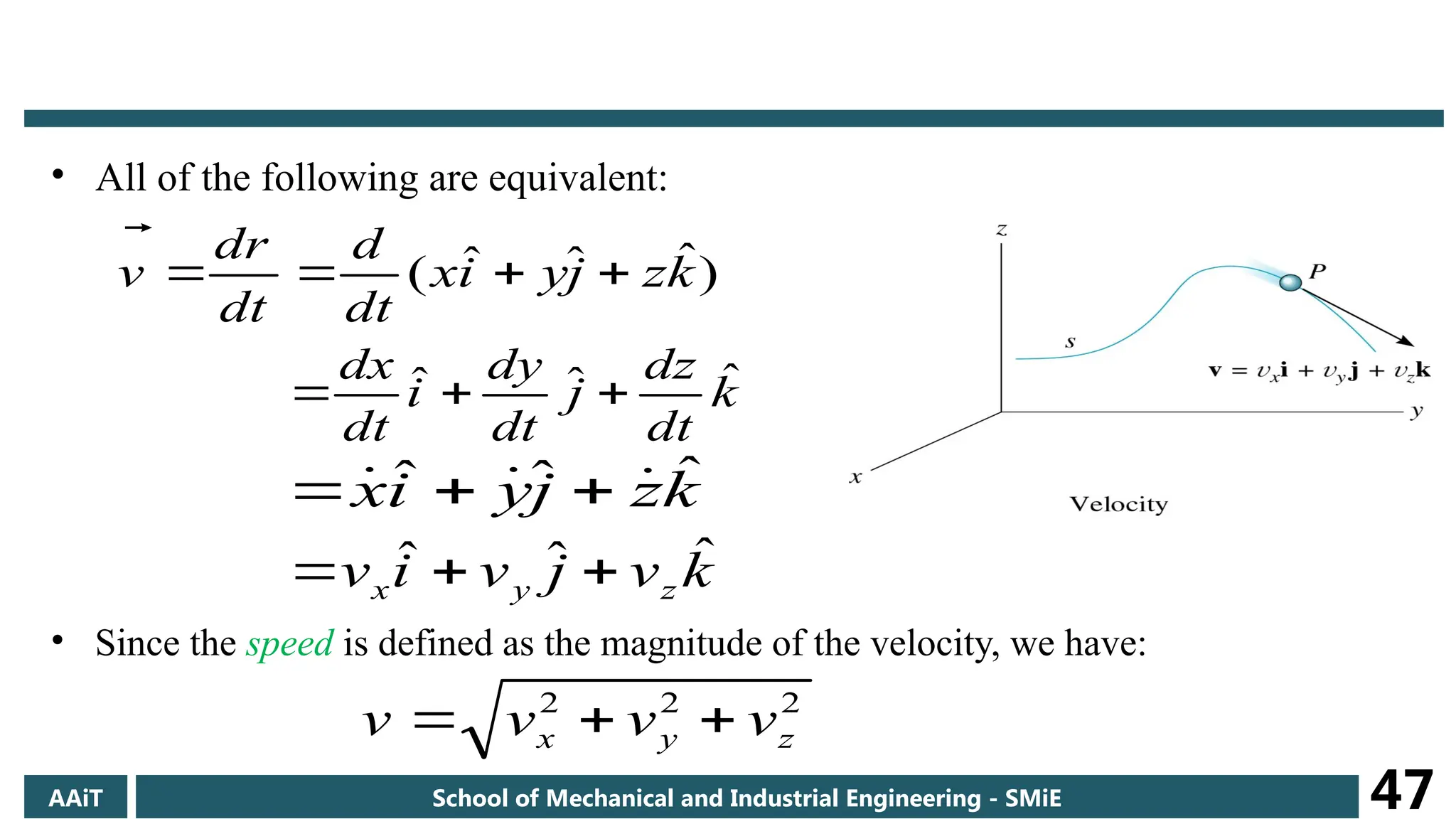
• All ofthe following are equivalent:
)
ˆ
ˆ
ˆ
( k
z
j
y
i
x
dt
d
dt
r
d
v
k
dt
dz
j
dt
dy
i
dt
dx ˆ
ˆ
ˆ
k
v
j
v
i
v z
y
x
ˆ
ˆ
ˆ
k
z
j
y
i
x ˆ
ˆ
ˆ
• Since the speed is defined as the magnitude of the velocity, we have:
2
2
2
z
y
x v
v
v
v
AAiT School of Mechanical and Industrial Engineering - SMiE 47
48.
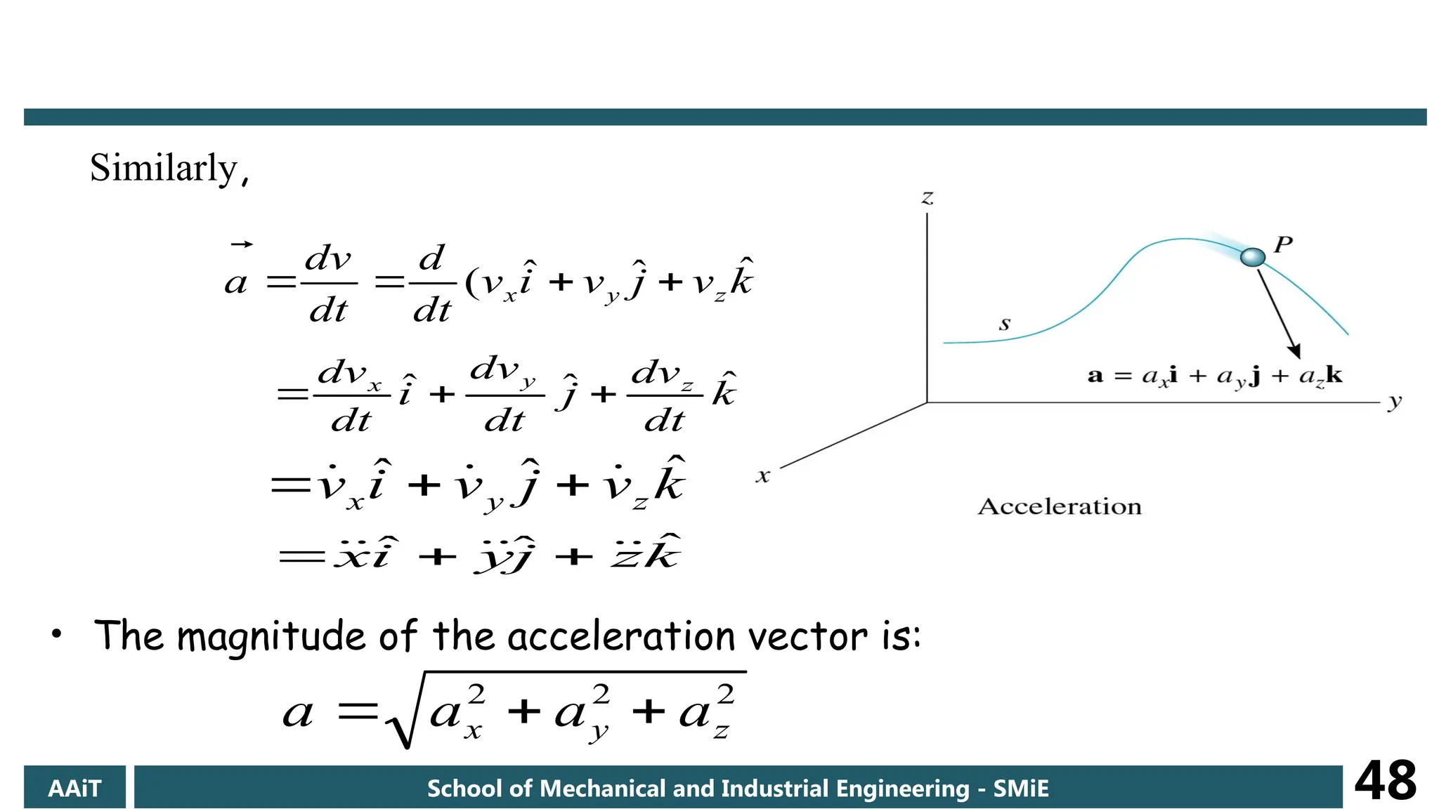
Similarly,
)
ˆ
ˆ
ˆ
( k
v
j
v
i
v
dt
d
dt
v
d
a z
y
x
k
dt
dv
j
dt
dv
i
dt
dv z
y
x ˆ
ˆ
ˆ
k
v
j
v
i
v z
y
x
ˆ
ˆ
ˆ
k
z
j
y
i
x ˆ
ˆ
ˆ
• The magnitude of the acceleration vector is:
2
2
2
z
y
x a
a
a
a
AAiT School of Mechanical and Industrial Engineering - SMiE 48
49.
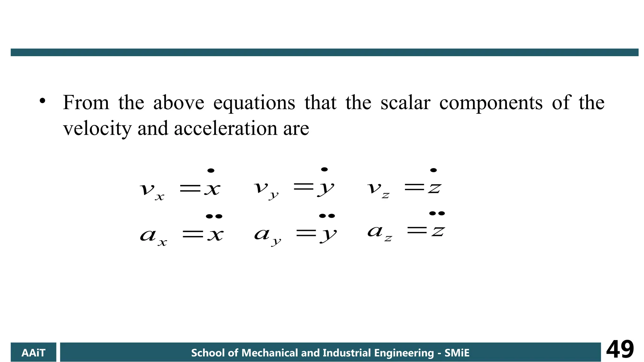
• From theabove equations that the scalar components of the
velocity and acceleration are
x
a
x
v
x
x
y
a
y
v
y
y
z
a
z
v
z
z
AAiT School of Mechanical and Industrial Engineering - SMiE 49
50.
• The useof rectangular components to describe the position,
the velocity and the acceleration of a particle is particularly
effective when the component ax of the acceleration depends
only upon t,x and/or vx, similarly for ay and az.
• The motion of the particle in the x direction, its motion in the y
direction, and its motion in the z direction can be considered
separately.
AAiT School of Mechanical and Industrial Engineering - SMiE 50
51.
• An importantapplication of two – dimensional kinematic
theory is the problem of projectile motion.
Assumptions
• Neglect the aerodynamic drag, the earth curvature and
rotation,
• The altitude range is so small enough so that the acceleration
due to gravity can be considered constant, therefore;
AAiT School of Mechanical and Industrial Engineering - SMiE 51
Projectile motion
52.
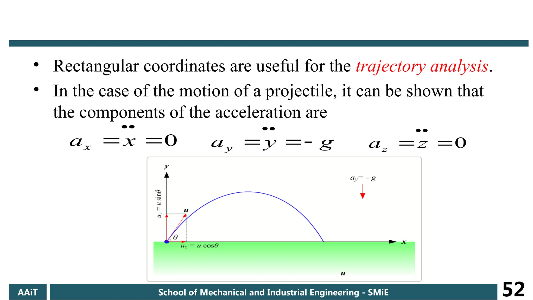
• Rectangular coordinatesare useful for the trajectory analysis.
• In the case of the motion of a projectile, it can be shown that
the components of the acceleration are
0
x
ax g
y
ay
0
z
az
AAiT School of Mechanical and Industrial Engineering - SMiE 52
53.
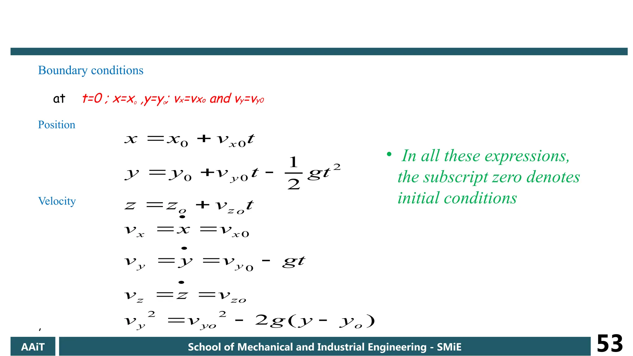
Boundary conditions
at t=0; x=x0 ,y=y0; vx=vxo and vy=vy0
Position
Velocity
,
t
v
z
z
gt
t
v
y
y
t
v
x
x
o
z
o
y
x
2
0
0
0
0
2
1
)
(
2
2
2
0
0
o
yo
y
zo
z
y
y
x
x
y
y
g
v
v
v
z
v
gt
v
y
v
v
x
v
• In all these expressions,
the subscript zero denotes
initial conditions
AAiT School of Mechanical and Industrial Engineering - SMiE 53
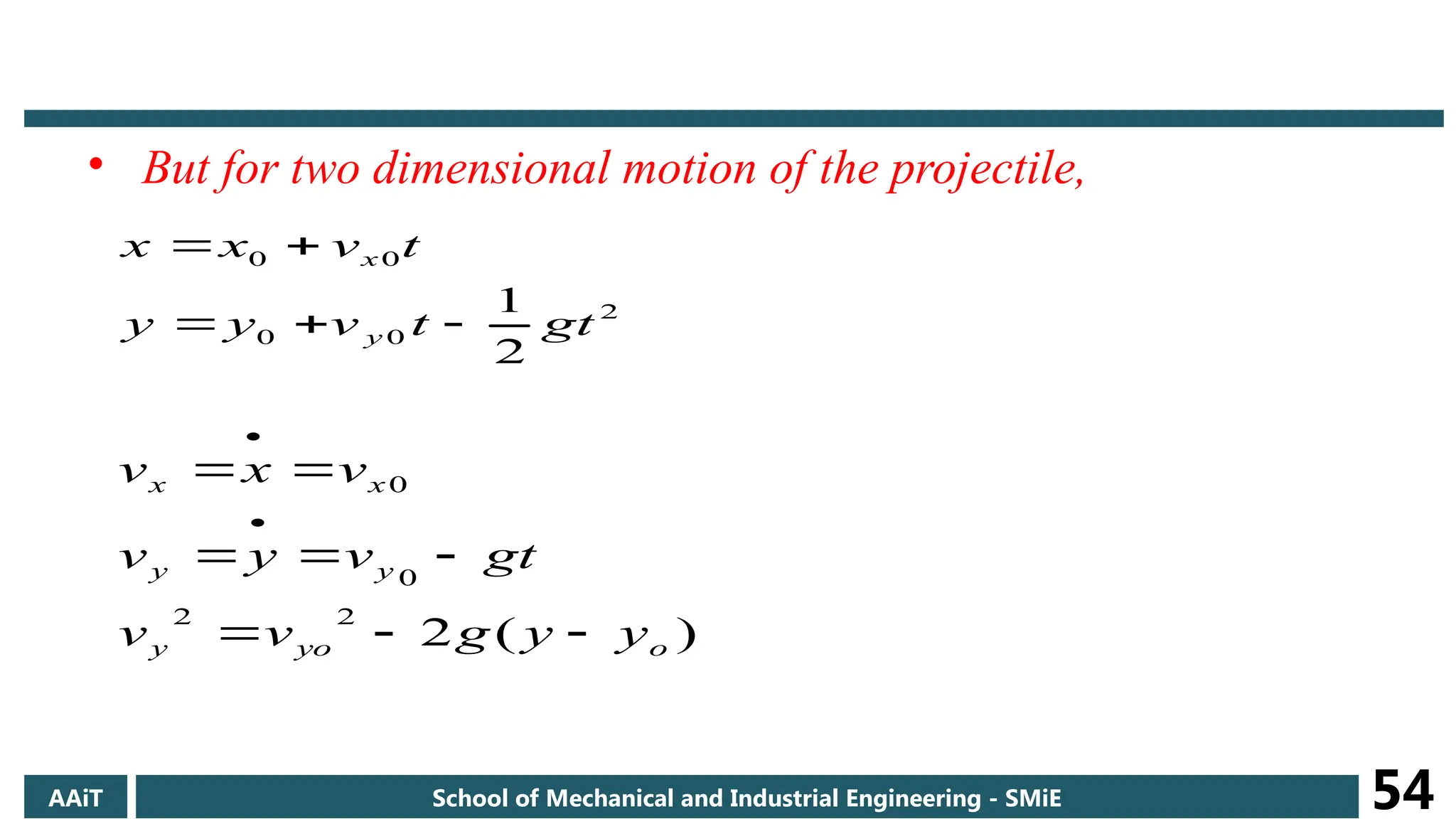
54.
• But fortwo dimensional motion of the projectile,
2
0
0
0
0
2
1
gt
t
v
y
y
t
v
x
x
y
x
)
(
2
2
2
0
0
o
yo
y
y
y
x
x
y
y
g
v
v
gt
v
y
v
v
x
v
AAiT School of Mechanical and Industrial Engineering - SMiE 54
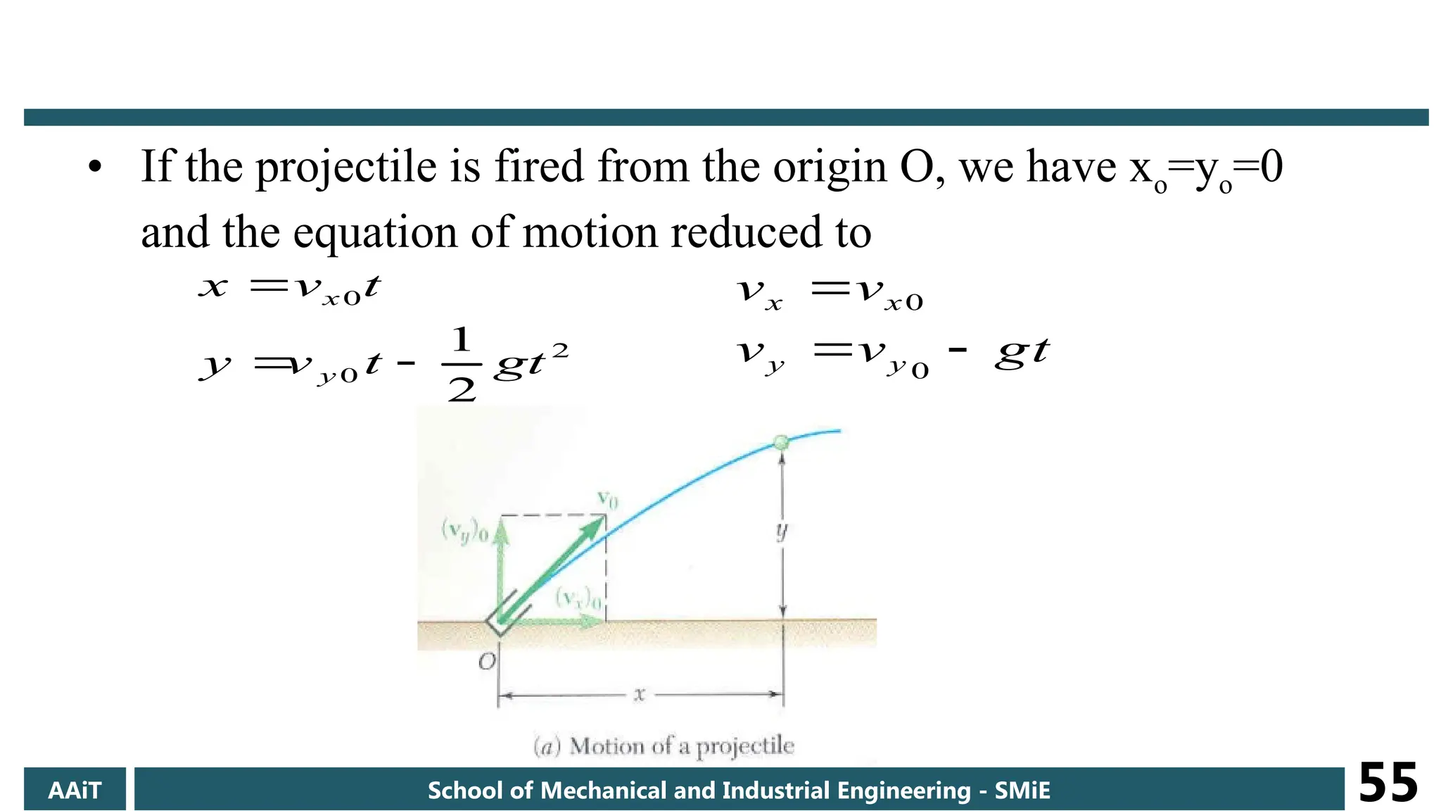
55.
• If theprojectile is fired from the origin O, we have xo=yo=0
and the equation of motion reduced to
2
0
0
2
1
gt
t
v
y
t
v
x
y
x
gt
v
v
v
v
y
y
x
x
0
0
AAiT School of Mechanical and Industrial Engineering - SMiE 55
56.
AAiT School ofMechanical and Industrial Engineering - SMiE 56
57.
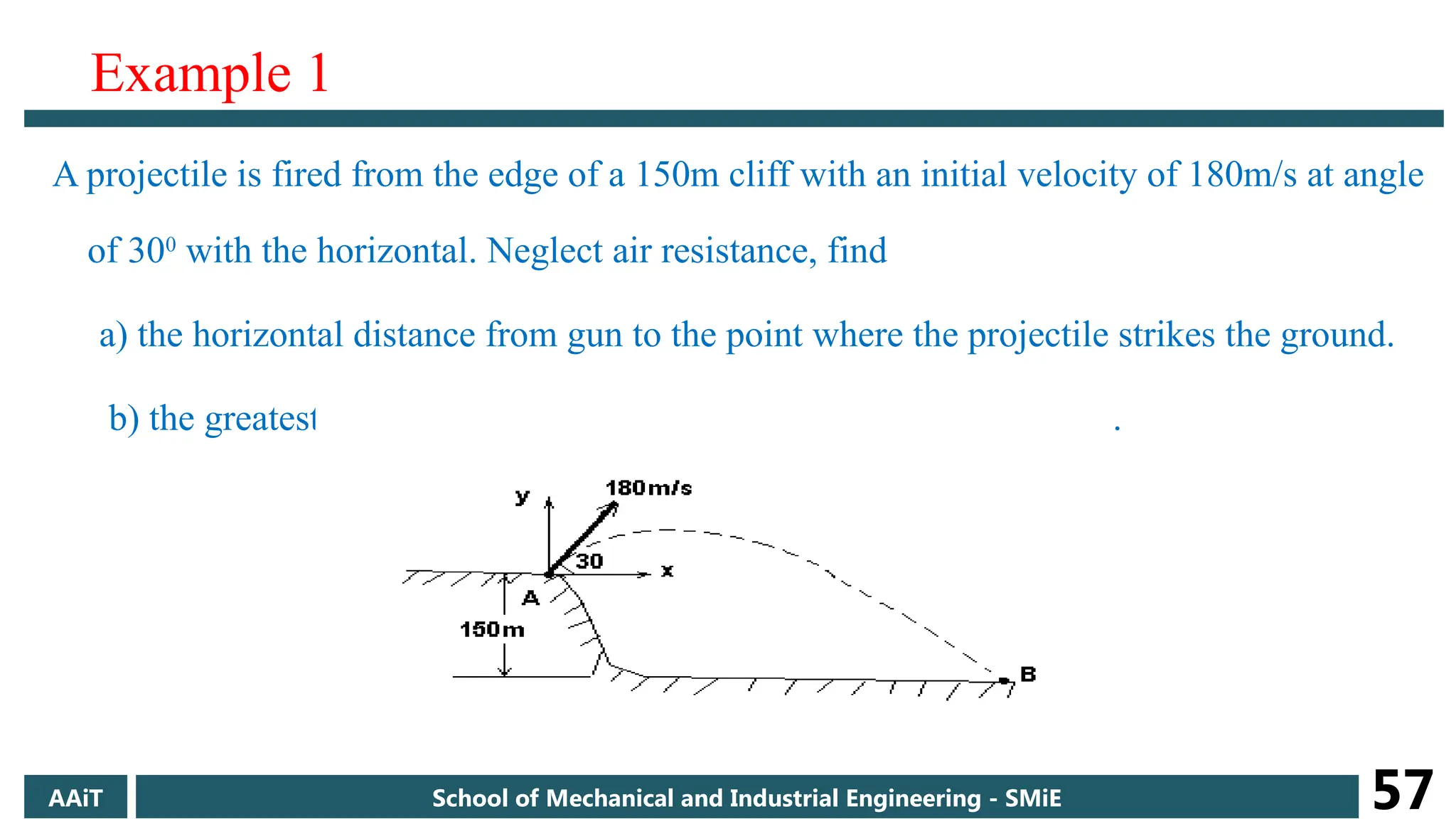
Example 1
A projectileis fired from the edge of a 150m cliff with an initial velocity of 180m/s at angle
of 300
with the horizontal. Neglect air resistance, find
a) the horizontal distance from gun to the point where the projectile strikes the ground.
b) the greatest elevation above the ground reached by the projectile.
AAiT School of Mechanical and Industrial Engineering - SMiE 57
58.
AAiT School ofMechanical and Industrial Engineering - SMiE 58
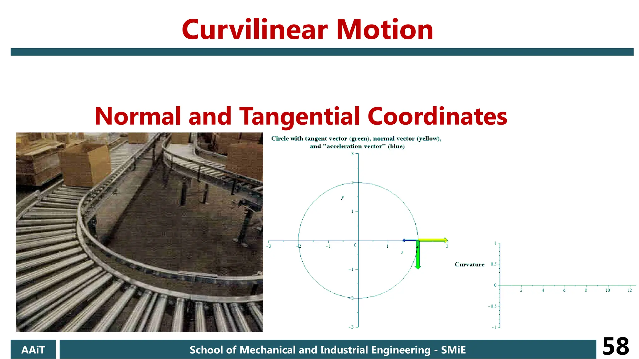
Curvilinear Motion
Normal and Tangential Coordinates
59.
• When aparticle moves along a curved path, it is sometimes
convenient to describe its motion using coordinates other than
Cartesian.
• When the path of motion is known, normal (n) and tangential (t)
coordinates are often used.
• They are path variables, which are measurements made along the
tangent t and normal n to the path of the particle.
• They are considered to move along the path with the particle.
• In the n-t coordinate system, the origin is located on the particle
(the origin moves with the particle).
AAiT School of Mechanical and Industrial Engineering - SMiE 59
60.
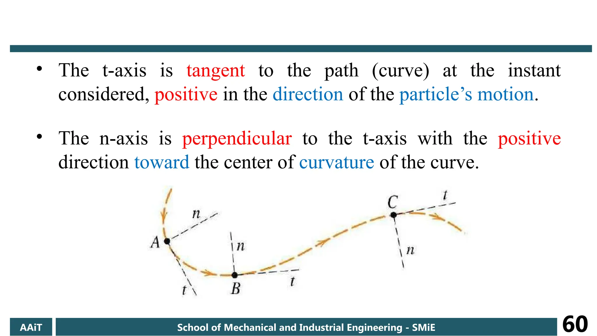
• The t-axisis tangent to the path (curve) at the instant
considered, positive in the direction of the particle’s motion.
• The n-axis is perpendicular to the t-axis with the positive
direction toward the center of curvature of the curve.
AAiT School of Mechanical and Industrial Engineering - SMiE 60
61.
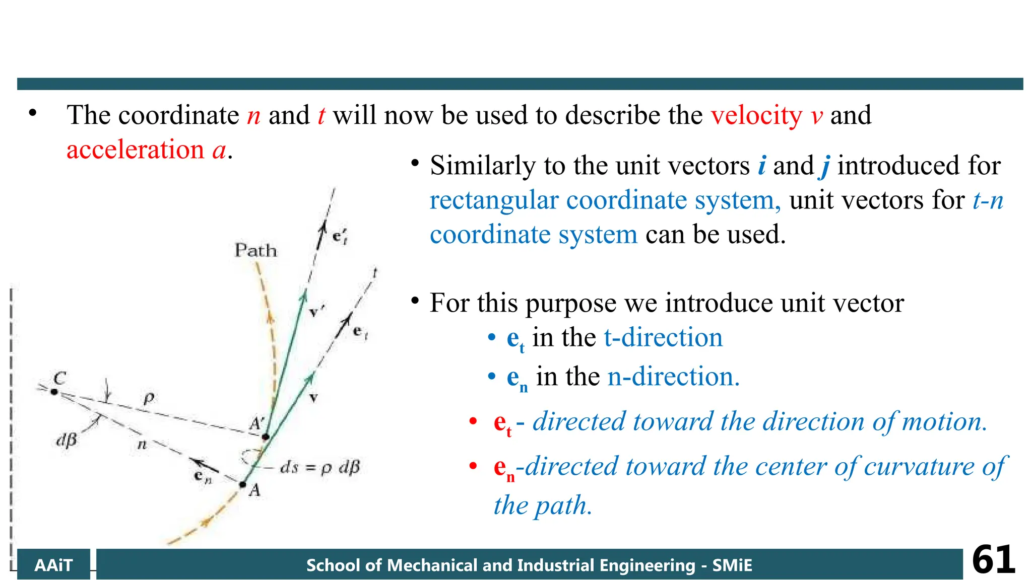
• The coordinaten and t will now be used to describe the velocity v and
acceleration a.
• Similarly to the unit vectors i and j introduced for
rectangular coordinate system, unit vectors for t-n
coordinate system can be used.
• For this purpose we introduce unit vector
• et in the t-direction
• en in the n-direction.
• et - directed toward the direction of motion.
• en-directed toward the center of curvature of
the path.
AAiT School of Mechanical and Industrial Engineering - SMiE 61
62.
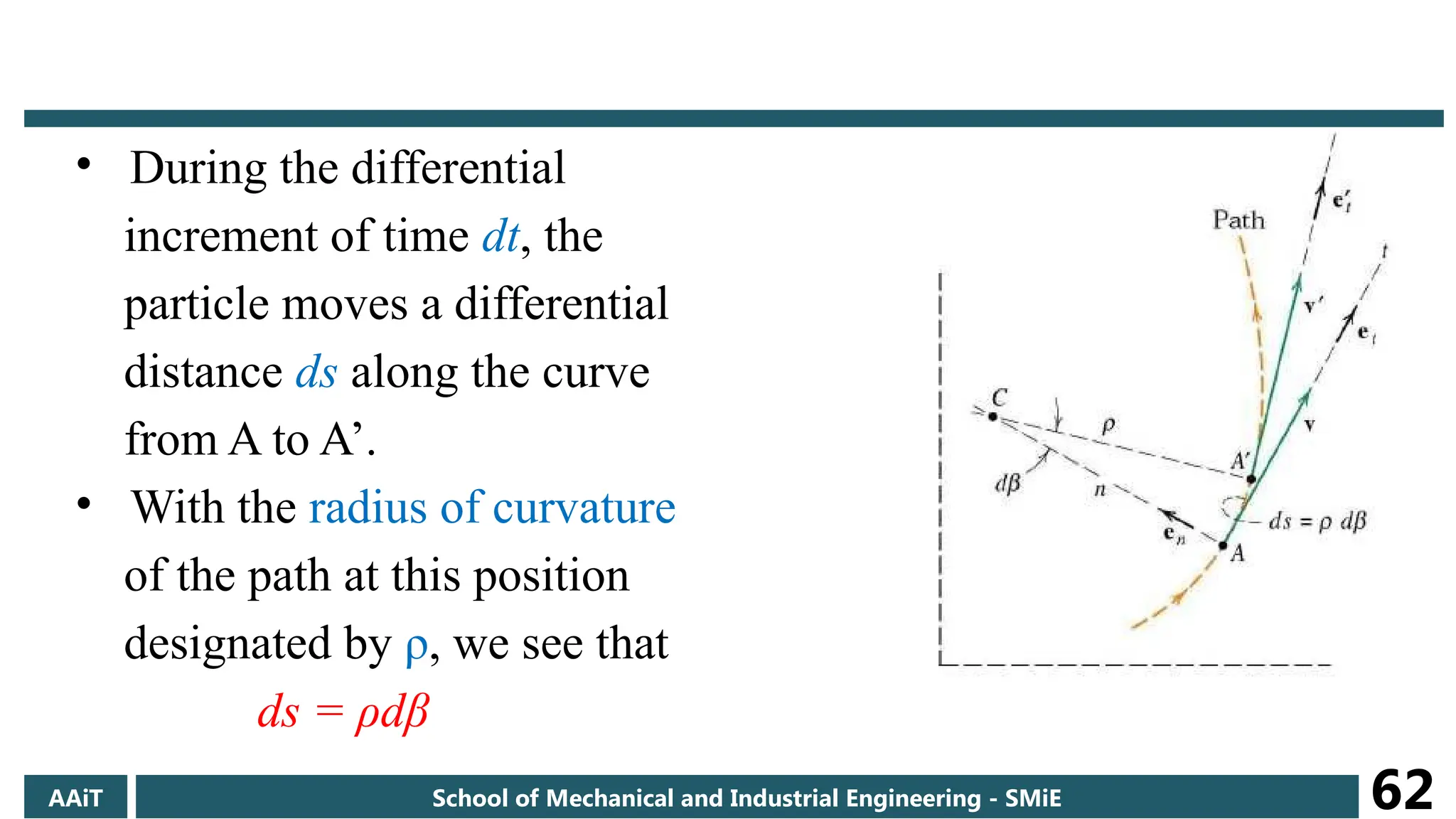
• During thedifferential
increment of time dt, the
particle moves a differential
distance ds along the curve
from A to A’.
• With the radius of curvature
of the path at this position
designated by ρ, we see that
ds = ρdβ
AAiT School of Mechanical and Industrial Engineering - SMiE 62
63.
velocity
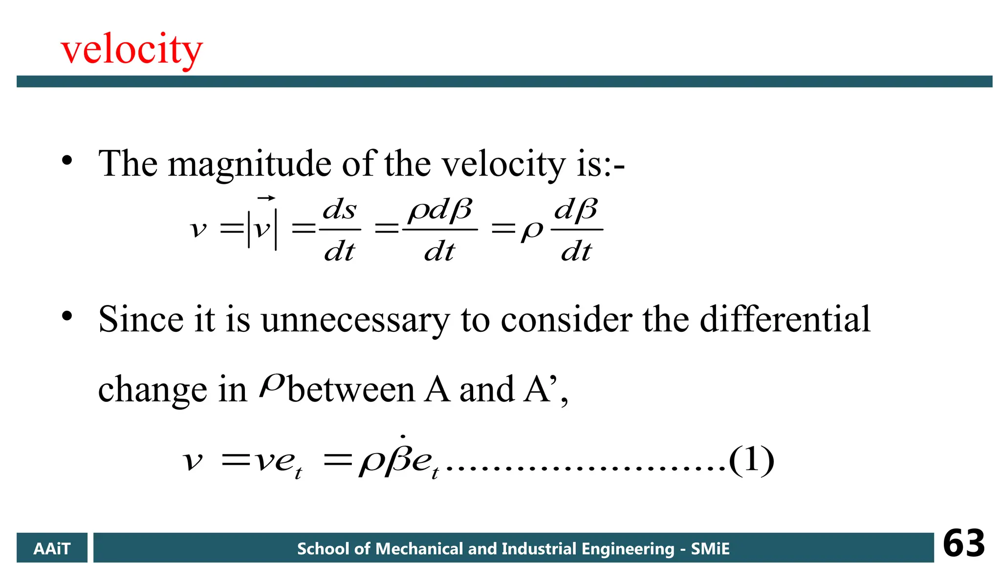
• The magnitudeof the velocity is:-
• Since it is unnecessary to consider the differential
change in between A and A’,
dt
d
dt
d
dt
ds
v
v
)
1
....(
..........
..........
t
t e
e
v
v
AAiT School of Mechanical and Industrial Engineering - SMiE 63
64.
Acceleration
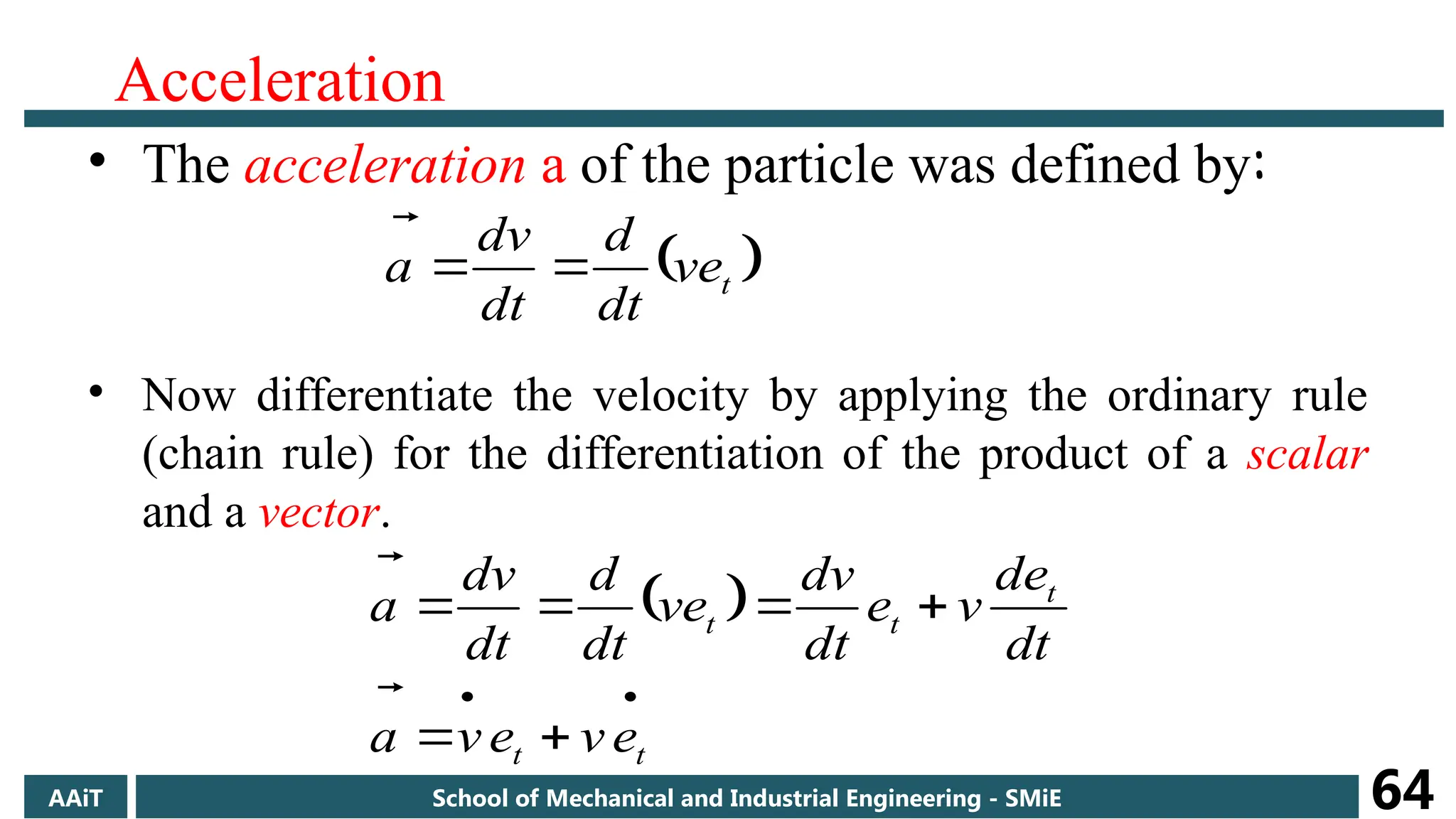
• The accelerationa of the particle was defined by:
• Now differentiate the velocity by applying the ordinary rule
(chain rule) for the differentiation of the product of a scalar
and a vector.
t
ve
dt
d
dt
dv
a
t
t
t
t
t
e
v
e
v
a
dt
de
v
e
dt
dv
ve
dt
d
dt
dv
a
AAiT School of Mechanical and Industrial Engineering - SMiE 64
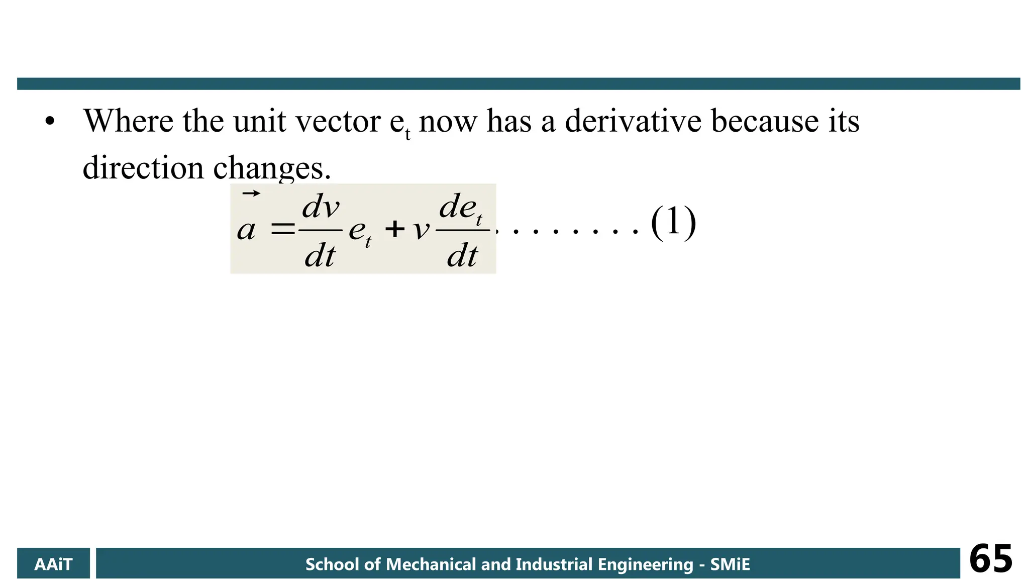
65.
• Where theunit vector et now has a derivative because its
direction changes.
. . . . . . . . . . . (1)
dt
de
v
e
dt
dv
a t
t
AAiT School of Mechanical and Industrial Engineering - SMiE 65
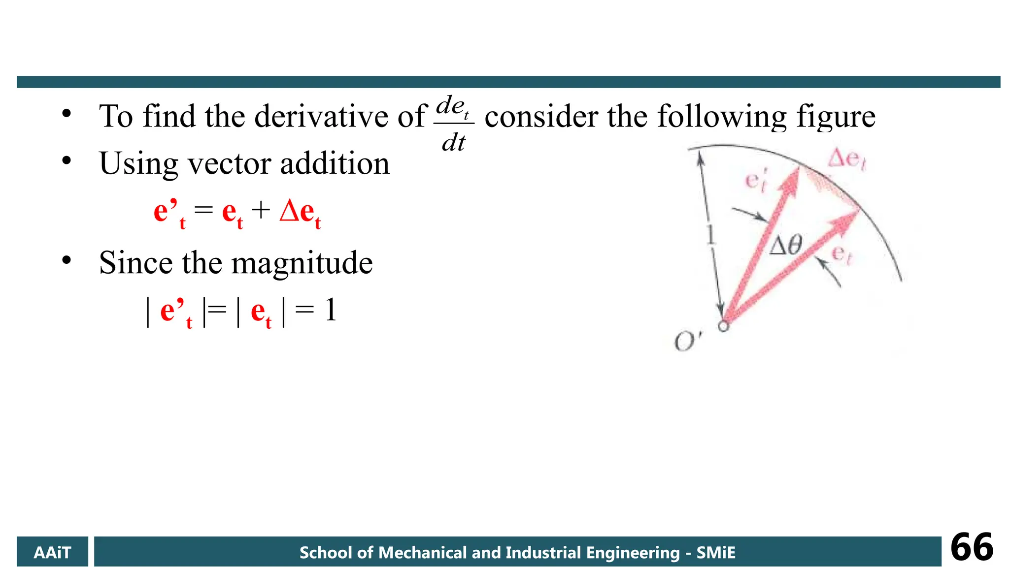
66.
• To findthe derivative of consider the following figure
• Using vector addition
e’t = et + ∆et
• Since the magnitude
| e’t |= | et | = 1
dt
det
AAiT School of Mechanical and Industrial Engineering - SMiE 66
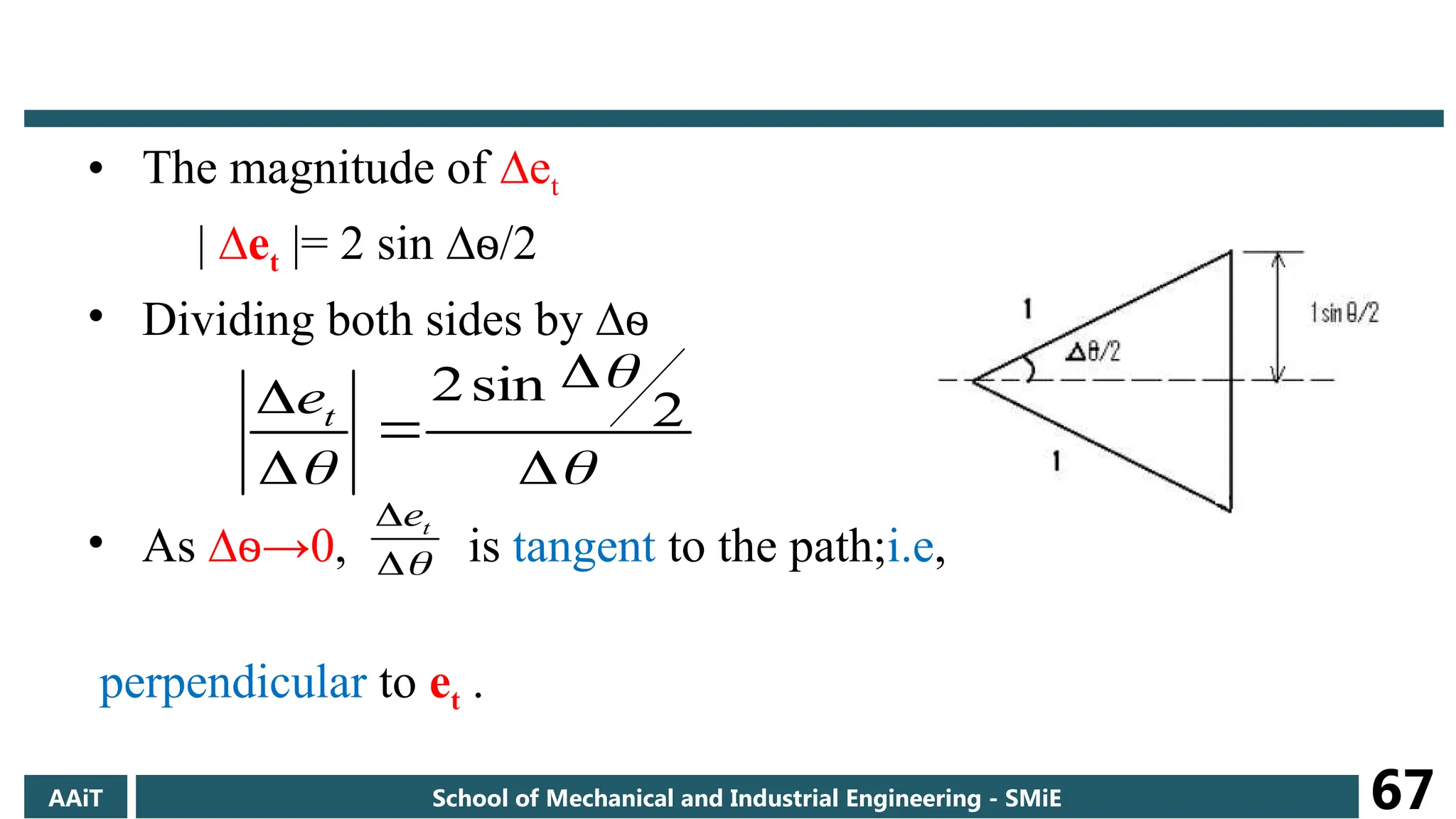
67.
• The magnitudeof ∆et
| ∆et |= 2 sin ∆ѳ/2
• Dividing both sides by ∆ѳ
• As ∆ →
ѳ 0, is tangent to the path;i.e,
perpendicular to et .
2
sin
2
t
e
t
e
AAiT School of Mechanical and Industrial Engineering - SMiE 67
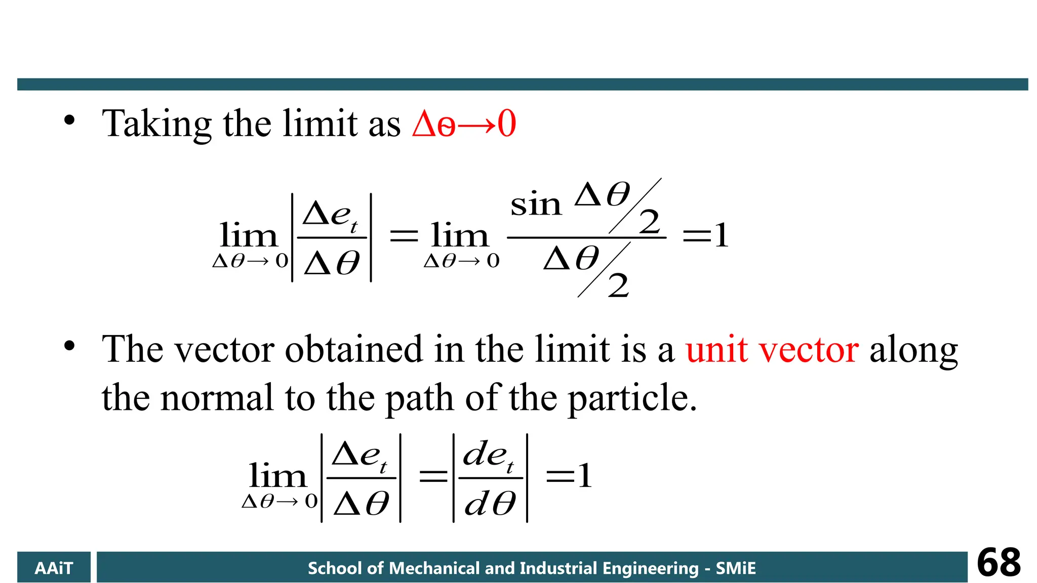
68.
• Taking thelimit as ∆ →
ѳ 0
• The vector obtained in the limit is a unit vector along
the normal to the path of the particle.
1
2
2
sin
lim
lim
0
0
t
e
1
lim
0
d
de
e t
t
AAiT School of Mechanical and Industrial Engineering - SMiE 68
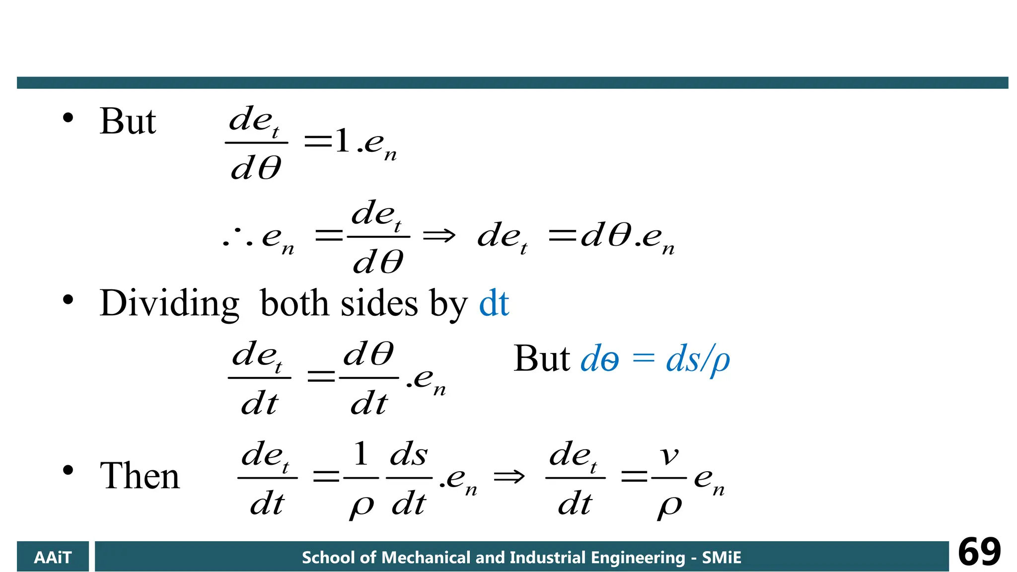
69.
• But
• Dividingboth sides by dt
But dѳ = ds/ρ
• Then
n
t
t
n
n
t
e
d
de
d
de
e
e
d
de
.
.
1
n
t
e
dt
d
dt
de
.
n
t
n
t
e
v
dt
de
e
dt
ds
dt
de
.
1
AAiT School of Mechanical and Industrial Engineering - SMiE 69
70.
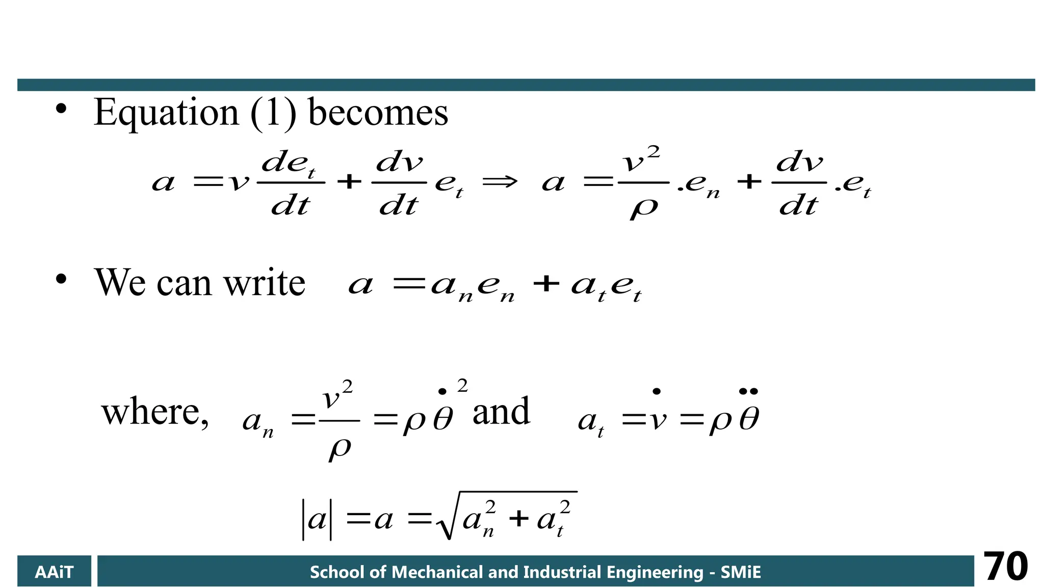
• Equation (1)becomes
• We can write
where, and
t
n
t
t
e
dt
dv
e
v
a
e
dt
dv
dt
de
v
a .
.
2
t
t
n
n e
a
e
a
a
2
2
v
an
v
at
2
2
t
n a
a
a
a
AAiT School of Mechanical and Industrial Engineering - SMiE 70
71.
Note:
• an isalways directed towards the center of curvature of the path.
• at is directed towards the positive t-direction of the motion if the
speed v is increasing and towards the negative t-direction if the
speed v is decreasing.
• At the inflection point in the curve, the normal acceleration,
goes to zero since ρ becomes infinity.
2
v
AAiT School of Mechanical and Industrial Engineering - SMiE 71
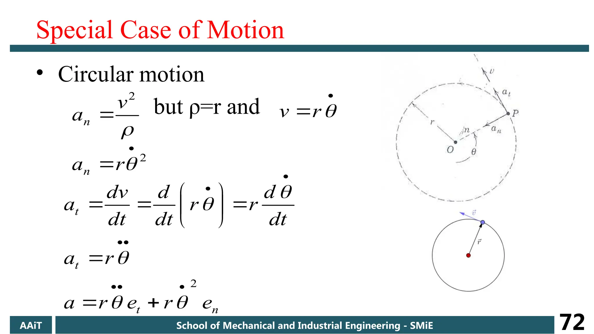
72.
Special Case ofMotion
• Circular motion
but ρ=r and
2
v
an
r
v
2
r
an
n
t
t
t
e
r
e
r
a
r
a
dt
d
r
r
dt
d
dt
dv
a
2
AAiT School of Mechanical and Industrial Engineering - SMiE 72
73.
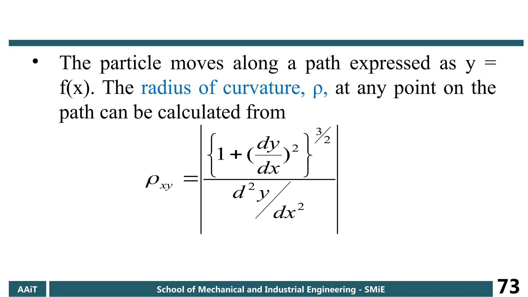
• The particlemoves along a path expressed as y =
f(x). The radius of curvature, ρ, at any point on the
path can be calculated from
2
2
2
3
2
)
(
1
dx
y
d
dx
dy
xy
AAiT School of Mechanical and Industrial Engineering - SMiE 73
74.
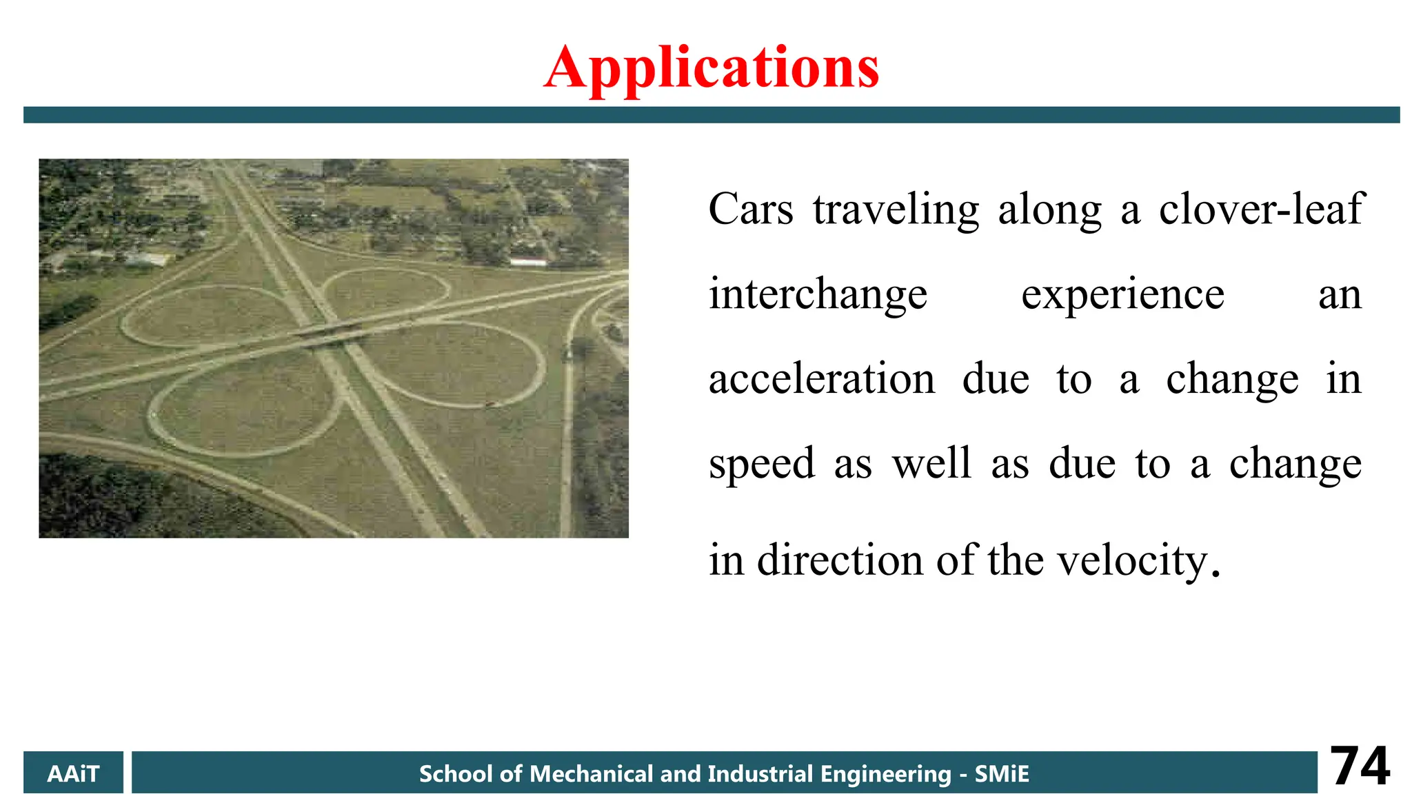
Applications
Cars traveling alonga clover-leaf
interchange experience an
acceleration due to a change in
speed as well as due to a change
in direction of the velocity.
AAiT School of Mechanical and Industrial Engineering - SMiE 74
75.
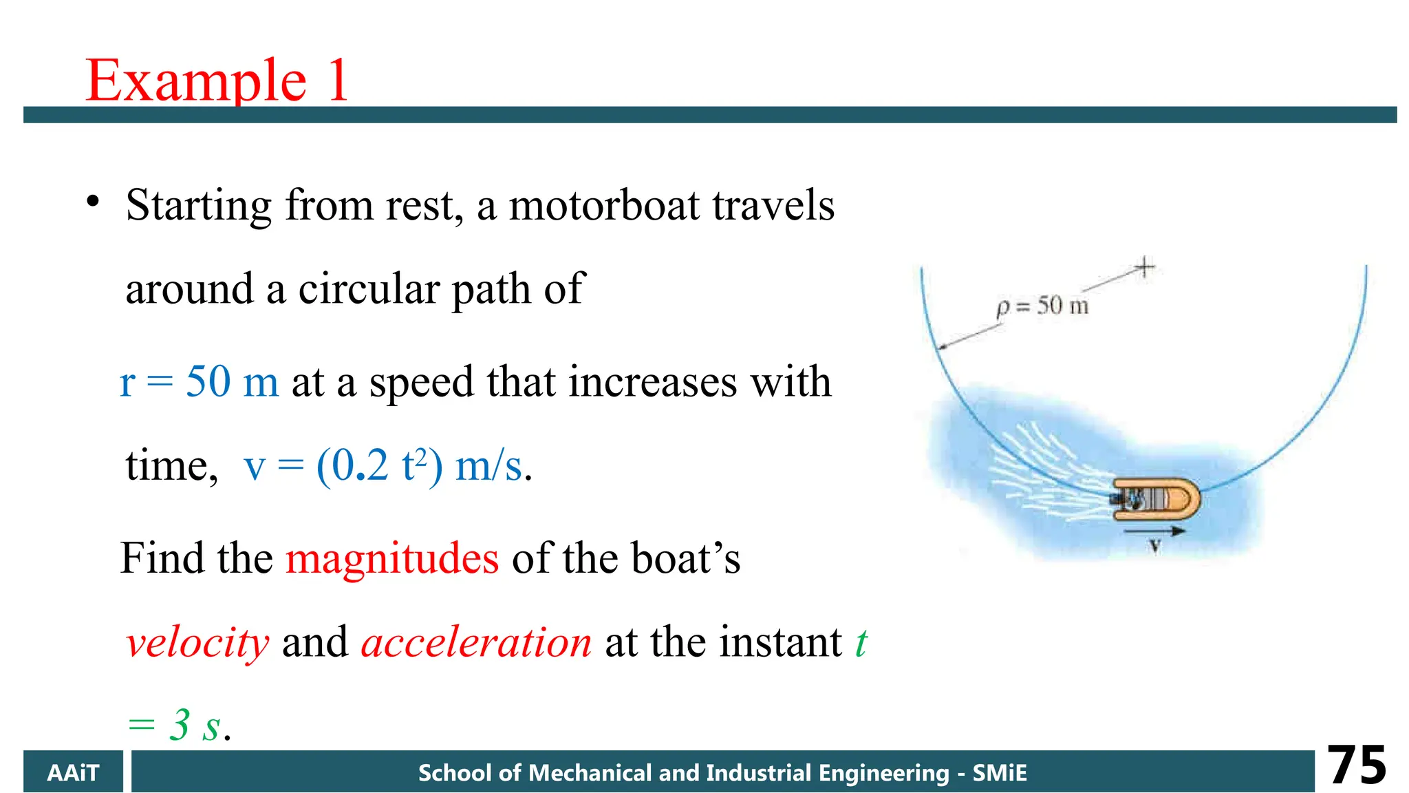
Example 1
• Startingfrom rest, a motorboat travels
around a circular path of
r = 50 m at a speed that increases with
time, v = (0.2 t2
) m/s.
Find the magnitudes of the boat’s
velocity and acceleration at the instant t
= 3 s.
AAiT School of Mechanical and Industrial Engineering - SMiE 75
76.
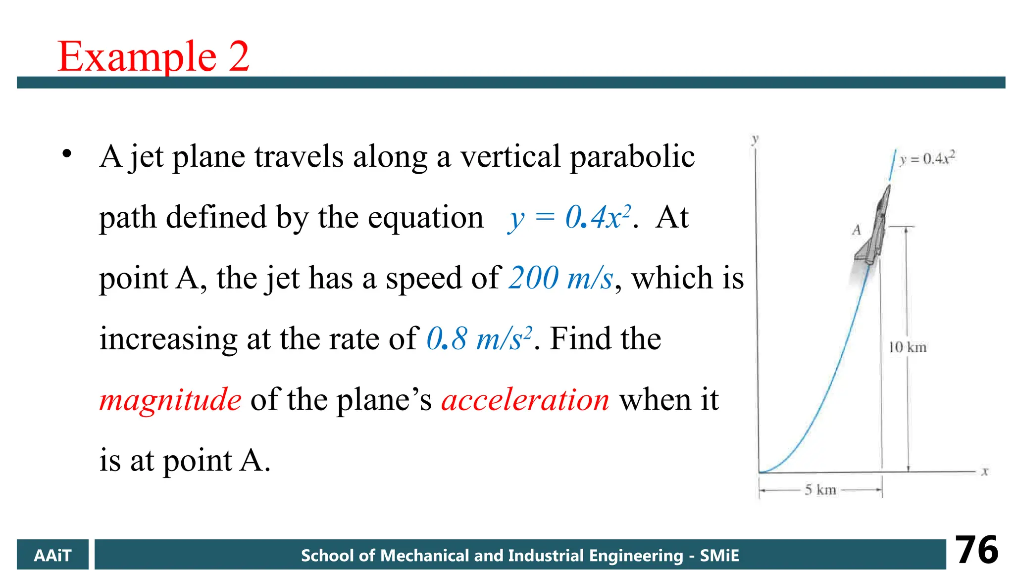
Example 2
• Ajet plane travels along a vertical parabolic
path defined by the equation y = 0.4x2
. At
point A, the jet has a speed of 200 m/s, which is
increasing at the rate of 0.8 m/s2
. Find the
magnitude of the plane’s acceleration when it
is at point A.
AAiT School of Mechanical and Industrial Engineering - SMiE 76
77.
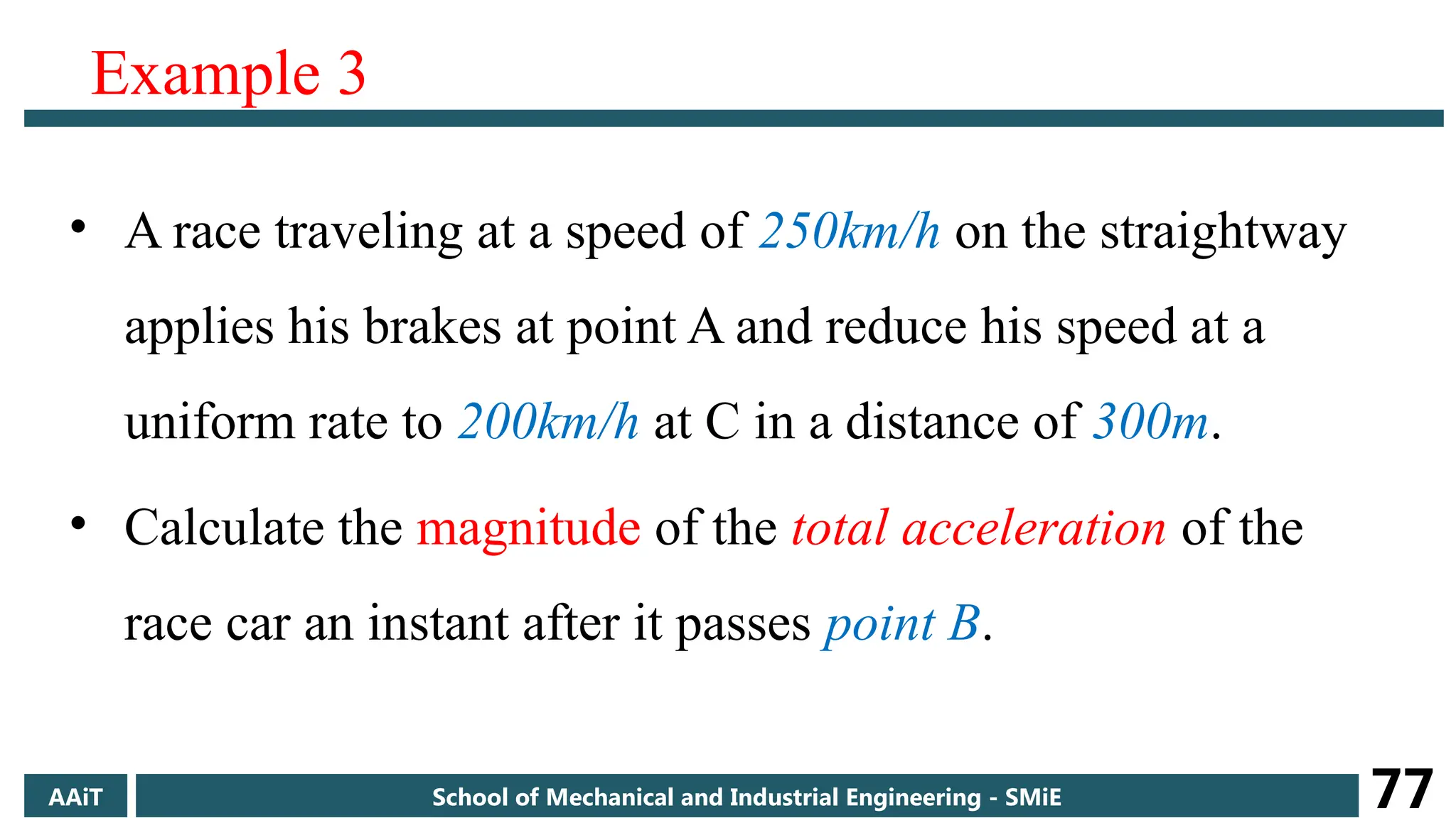
Example 3
• Arace traveling at a speed of 250km/h on the straightway
applies his brakes at point A and reduce his speed at a
uniform rate to 200km/h at C in a distance of 300m.
• Calculate the magnitude of the total acceleration of the
race car an instant after it passes point B.
AAiT School of Mechanical and Industrial Engineering - SMiE 77
78.
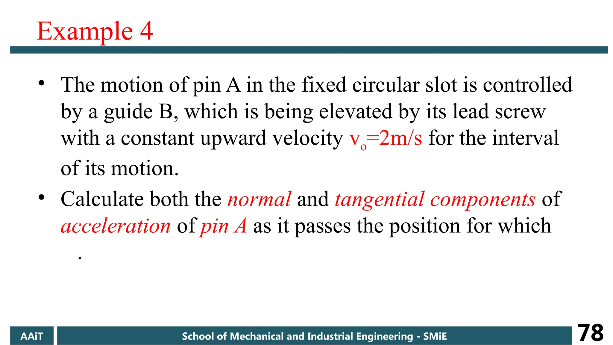
Example 4
• Themotion of pin A in the fixed circular slot is controlled
by a guide B, which is being elevated by its lead screw
with a constant upward velocity vo=2m/s for the interval
of its motion.
• Calculate both the normal and tangential components of
acceleration of pin A as it passes the position for which
.
AAiT School of Mechanical and Industrial Engineering - SMiE 78
79.
AAiT School ofMechanical and Industrial Engineering - SMiE 79
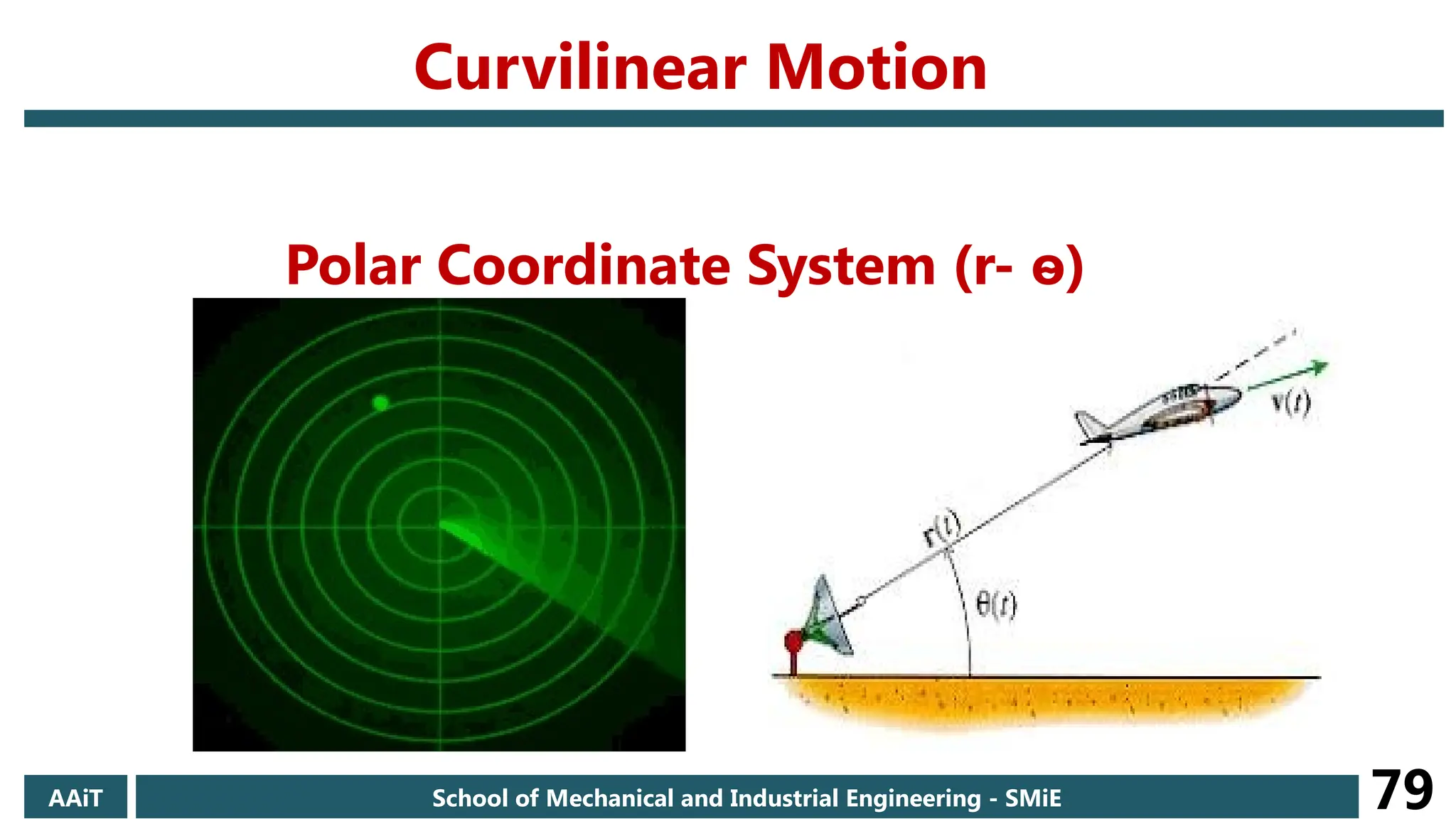
Curvilinear Motion
Polar Coordinate System (r- ѳ)
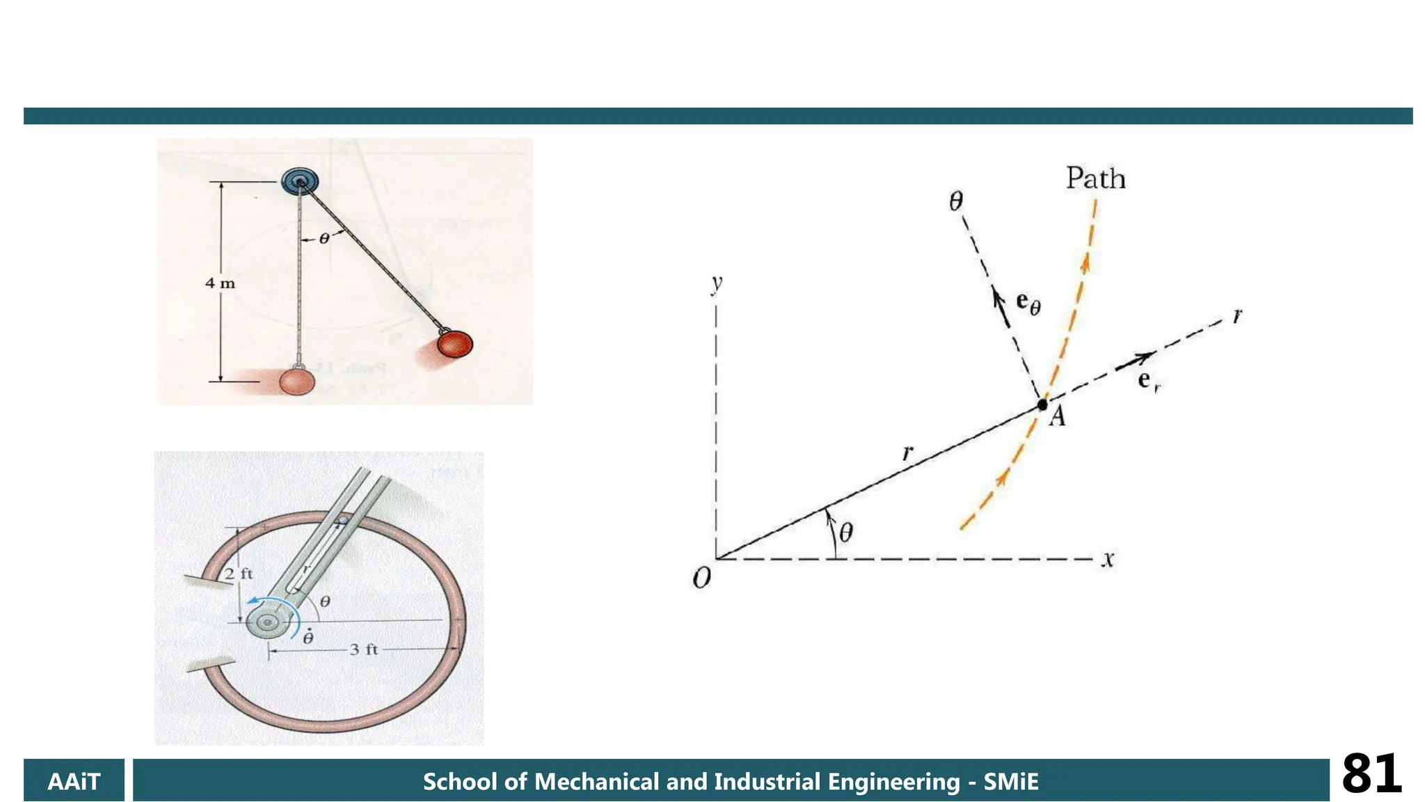
80.
• The thirddescription for plane curvilinear motion.
• Where the particle is located by the radial distance r from a fixed
pole and by an angular measurement ѳ to the radial line.
• Polar coordinates are particularly useful when a motion is
constrained through the control of a radial distance and an angular
position, or when an unconstrained motion is observed by
measurements of a radial distance and an angular position.
AAiT School of Mechanical and Industrial Engineering - SMiE 80
Polar Coordinate System (r- ѳ)
81.
AAiT School ofMechanical and Industrial Engineering - SMiE 81
82.
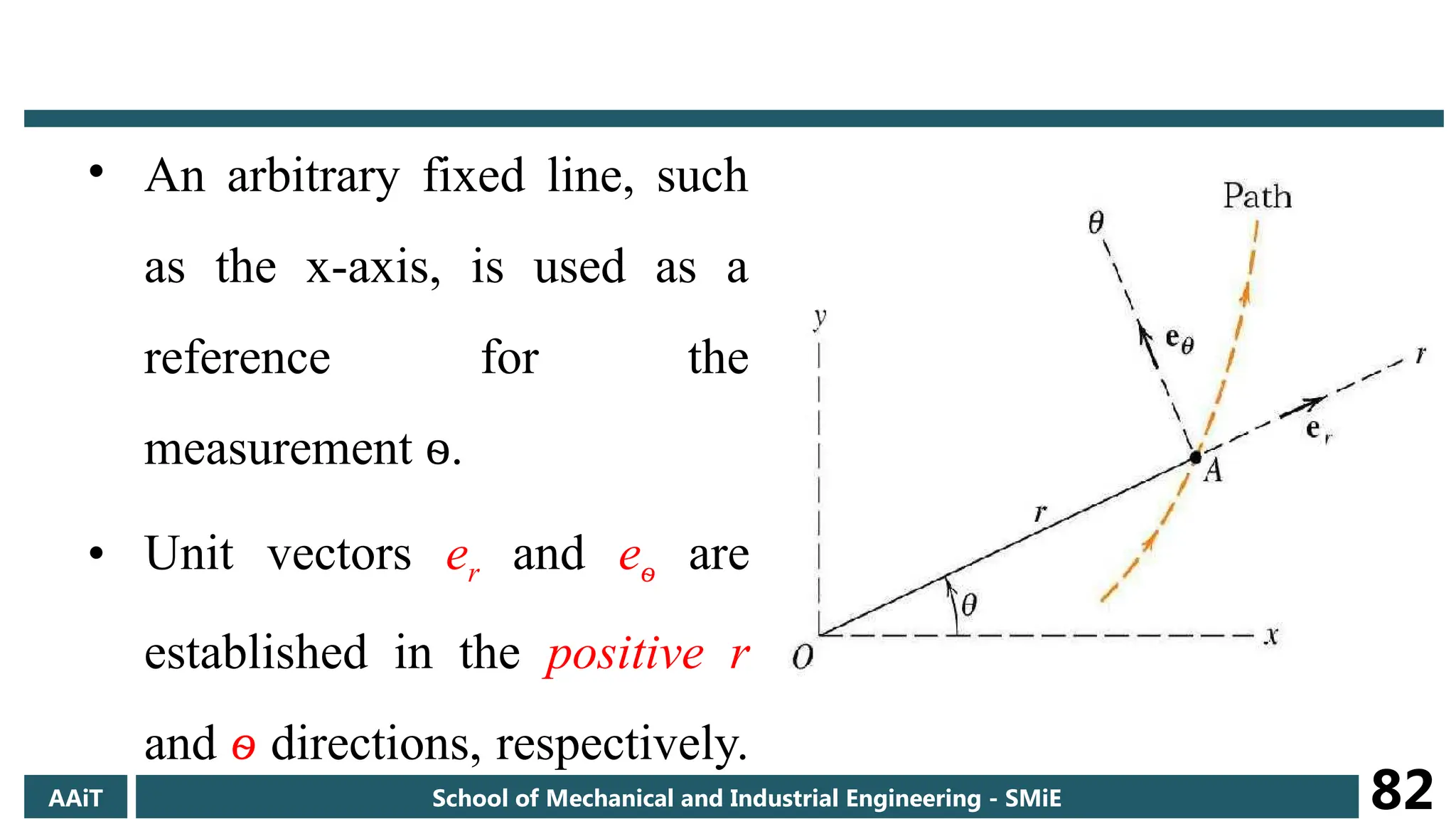
• An arbitraryfixed line, such
as the x-axis, is used as a
reference for the
measurement ѳ.
• Unit vectors er and eѳ are
established in the positive r
and ѳ directions, respectively.
AAiT School of Mechanical and Industrial Engineering - SMiE 82
83.
• The positionvector to the particle at A has a magnitude
equal to the radial distance r and a direction specified by
the unit vector er.
• We express the location of the particle at A by the vector
r
e
r.
r
•
r
AAiT School of Mechanical and Industrial Engineering - SMiE 83
84.
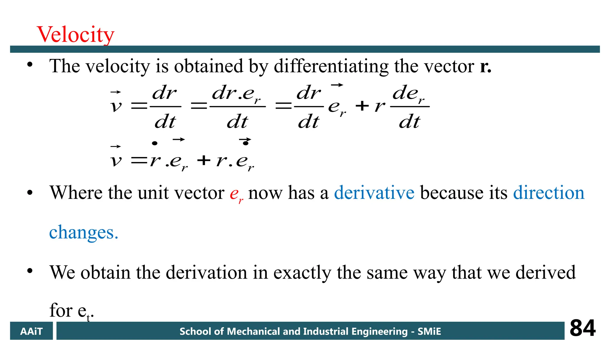
Velocity
• The velocityis obtained by differentiating the vector r.
• Where the unit vector er now has a derivative because its direction
changes.
• We obtain the derivation in exactly the same way that we derived
for et.
r
r
r
r
r
e
r
e
r
v
dt
e
d
r
e
dt
dr
dt
e
dr
dt
r
d
v
.
.
.
AAiT School of Mechanical and Industrial Engineering - SMiE 84
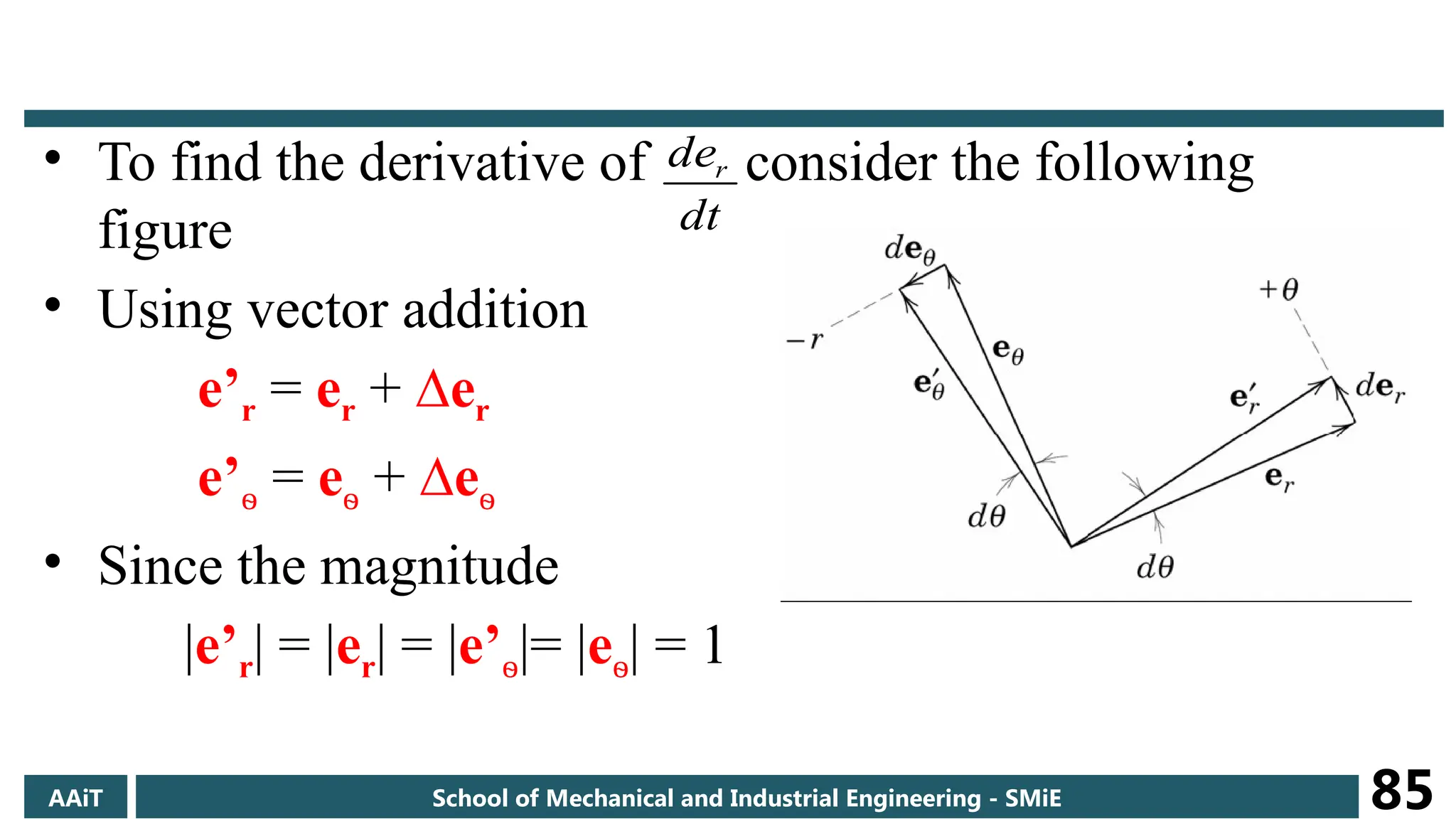
85.
• To findthe derivative of consider the following
figure
• Using vector addition
e’r = er + ∆er
e’ѳ = eѳ + ∆eѳ
• Since the magnitude
|e’r| = |er| = |e’ѳ|= |eѳ| = 1
dt
der
AAiT School of Mechanical and Industrial Engineering - SMiE 85
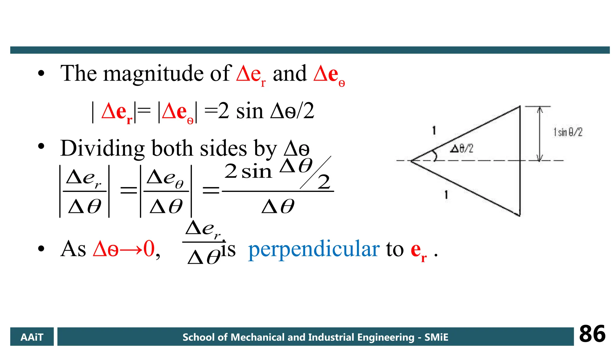
86.
• The magnitudeof ∆er and ∆eѳ
| ∆er|= |∆eѳ| =2 sin ∆ѳ/2
• Dividing both sides by ∆ѳ
• As ∆ →
ѳ 0, is perpendicular to er .
2
sin
2
e
er
r
e
AAiT School of Mechanical and Industrial Engineering - SMiE 86
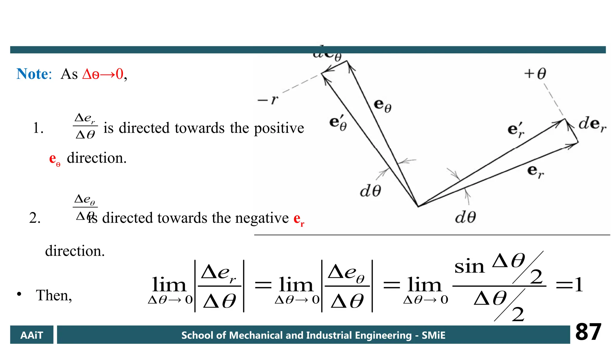
87.
Note: As ∆→
ѳ 0,
1. is directed towards the positive
eѳ direction.
2. is directed towards the negative er
direction.
• Then,
r
e
e
1
2
2
sin
lim
lim
lim
0
0
0
e
er
AAiT School of Mechanical and Industrial Engineering - SMiE 87
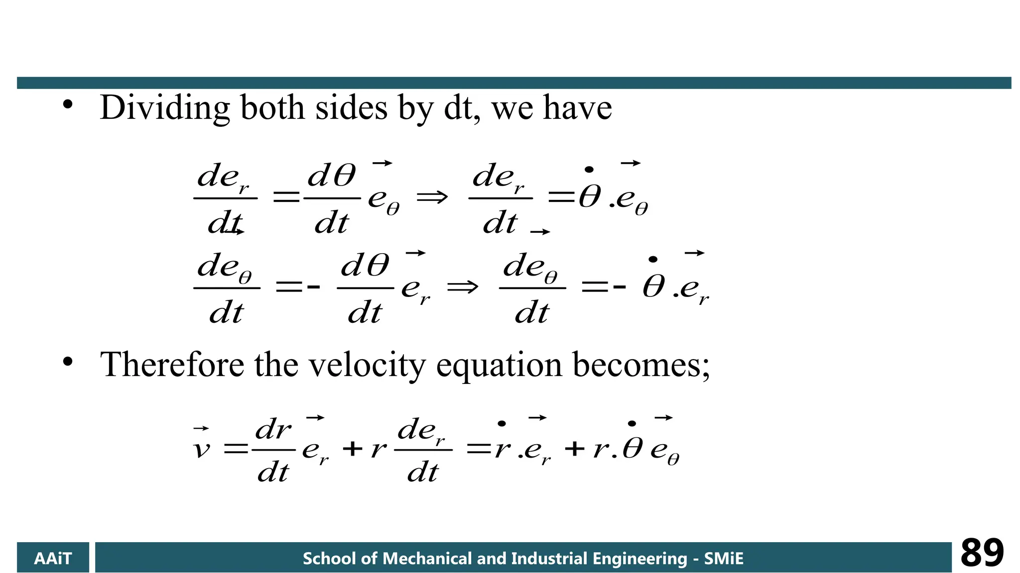
• Dividing bothsides by dt, we have
• Therefore the velocity equation becomes;
r
r
r
r
e
dt
e
d
e
dt
d
dt
e
d
e
dt
e
d
e
dt
d
dt
e
d
.
.
e
r
e
r
dt
e
d
r
e
dt
dr
v r
r
r
.
.
AAiT School of Mechanical and Industrial Engineering - SMiE 89
90.
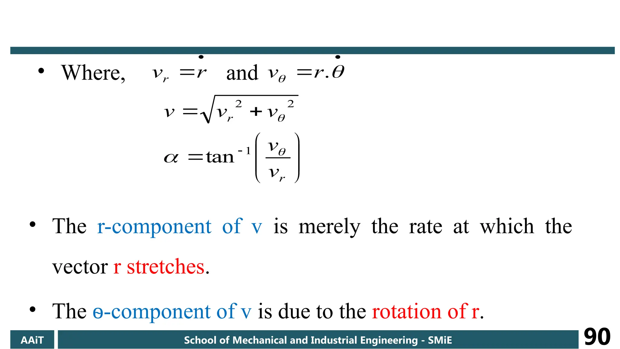
• Where, and
r
vr
.
r
v
r
r
v
v
v
v
v
1
2
2
tan
AAiT School of Mechanical and Industrial Engineering - SMiE 90
• The r-component of v is merely the rate at which the
vector r stretches.
• The ѳ-component of v is due to the rotation of r.
91.
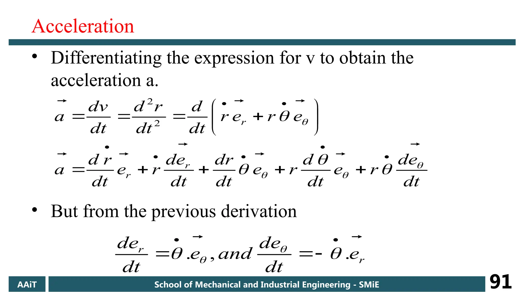
Acceleration
• Differentiating theexpression for v to obtain the
acceleration a.
• But from the previous derivation
dt
e
d
r
e
dt
d
r
e
dt
dr
dt
e
d
r
e
dt
r
d
a
e
r
e
r
dt
d
dt
r
d
dt
v
d
a
r
r
r
2
2
r
r
e
dt
de
and
e
dt
de
.
,
.
AAiT School of Mechanical and Industrial Engineering - SMiE 91
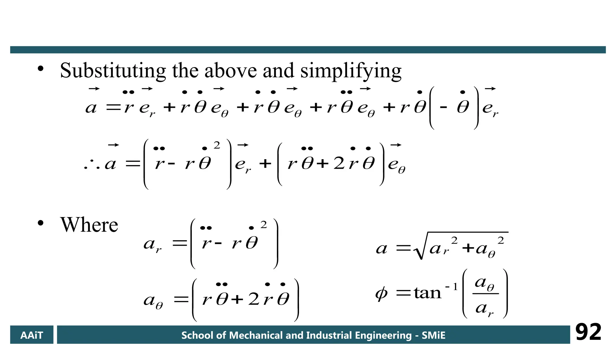
92.
• Substituting theabove and simplifying
• Where
e
r
r
e
r
r
a
e
r
e
r
e
r
e
r
e
r
a
r
r
r
2
2
r
r
a
r
r
ar
2
2
r
r
a
a
a
a
a
1
2
2
tan
AAiT School of Mechanical and Industrial Engineering - SMiE 92
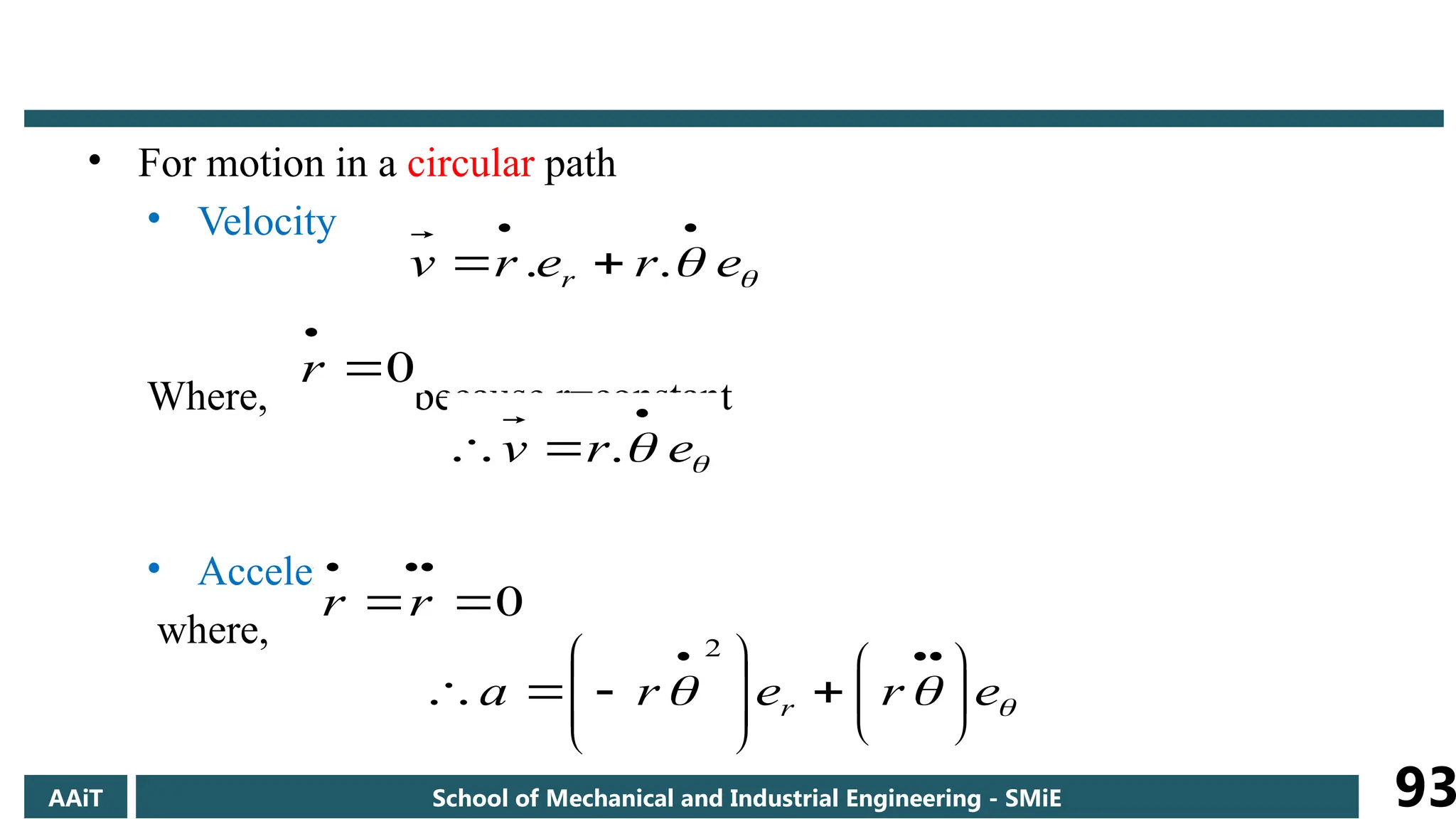
93.
• For motionin a circular path
• Velocity
Where, because r=constant
• Acceleration
where,
e
r
e
r
v r
.
.
0
r
e
r
v
.
0
r
r
e
r
e
r
a r
2
AAiT School of Mechanical and Industrial Engineering - SMiE 93
94.
AAiT School ofMechanical and Industrial Engineering - SMiE 94
Kinematics of
Particles
Relative Motion
95.
Relative motion
• Inthis portion Relative motion analysis : is the motion analysis of a
particle using moving reference system coordinate in reference to
fixed reference system.
• we will confine our attention to:-
– moving reference systems that translate but do not rotate.
– The relative motion analysis is limited to plane motion.
• Note: in this section we need
1. Inertial(fixed) frame of reference.
2. Translating(not rotating) frame of reference.
AAiT School of Mechanical and Industrial Engineering - SMiE 95
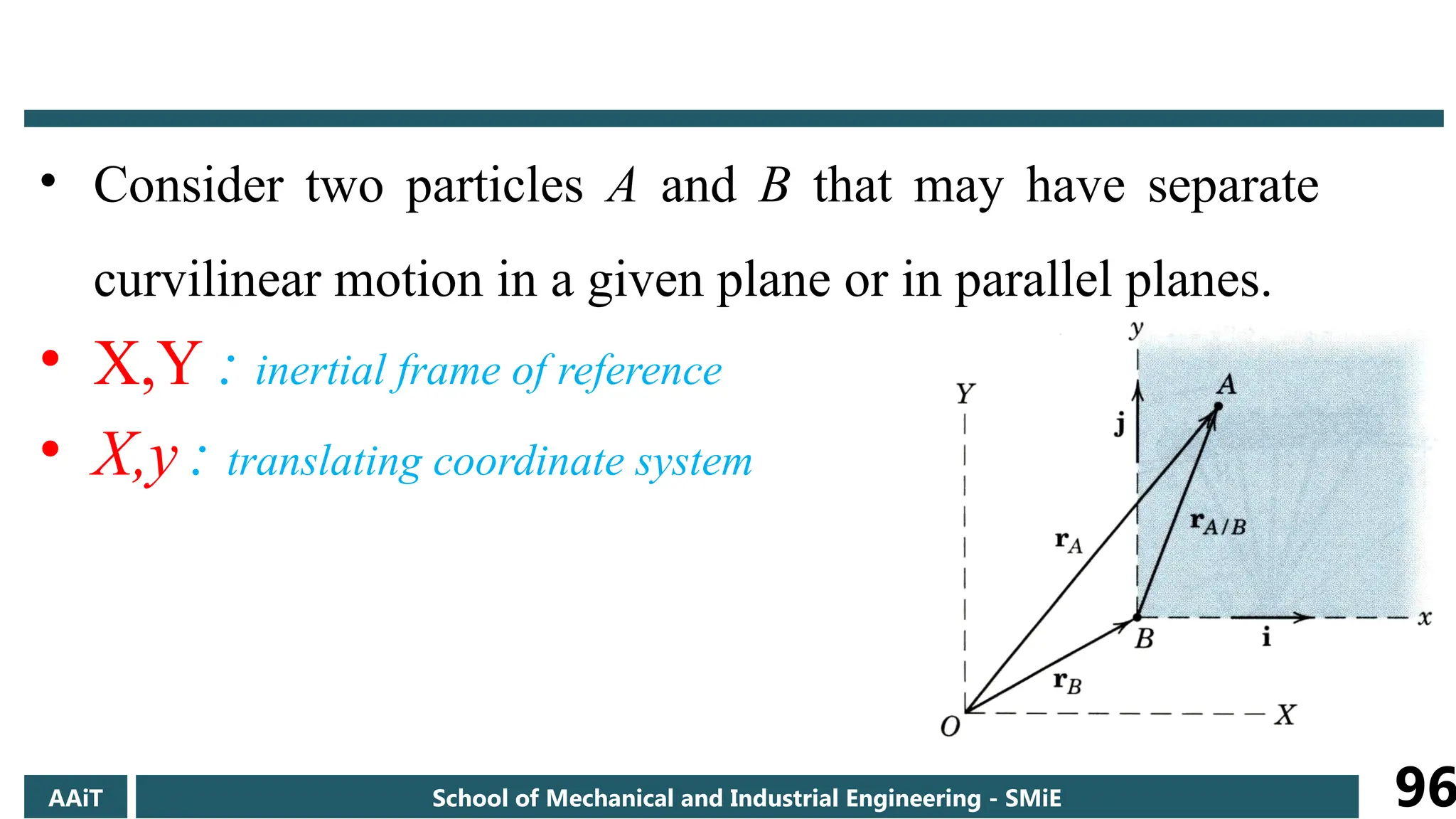
96.
• Consider twoparticles A and B that may have separate
curvilinear motion in a given plane or in parallel planes.
• X,Y : inertial frame of reference
• X,y : translating coordinate system
AAiT School of Mechanical and Industrial Engineering - SMiE 96
97.
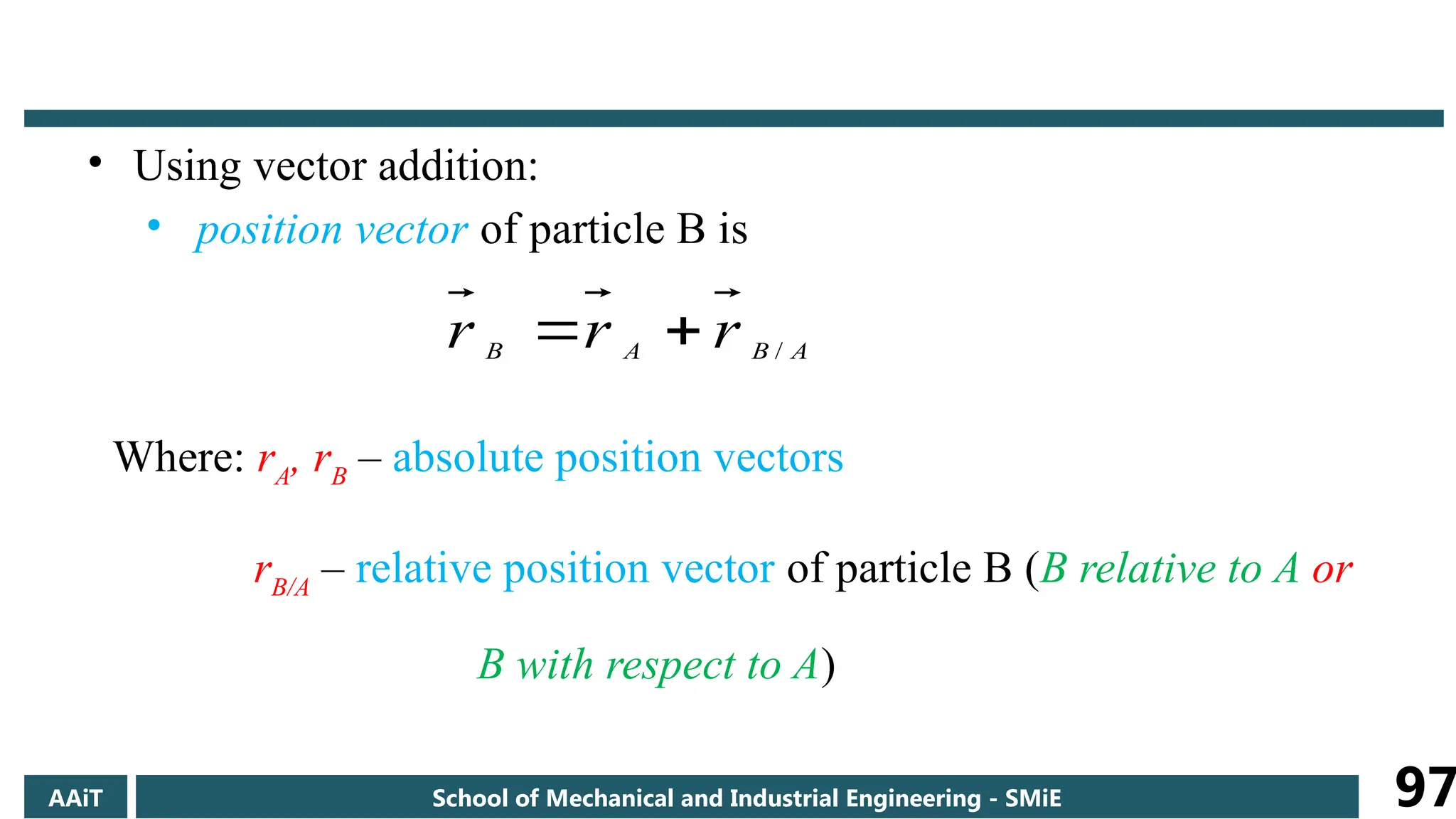
• Using vectoraddition:
• position vector of particle B is
Where: rA
, rB
– absolute position vectors
rB/A
– relative position vector of particle B (B relative to A or
B with respect to A)
A
B
A
B r
r
r /
AAiT School of Mechanical and Industrial Engineering - SMiE 97
98.
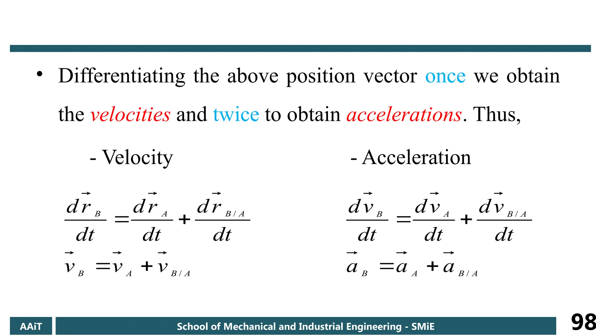
• Differentiating theabove position vector once we obtain
the velocities and twice to obtain accelerations. Thus,
- Velocity - Acceleration
A
B
A
B
A
B
A
B
v
v
v
dt
r
d
dt
r
d
dt
r
d
/
/
A
B
A
B
A
B
A
B
a
a
a
dt
v
d
dt
v
d
dt
v
d
/
/
AAiT School of Mechanical and Industrial Engineering - SMiE 98
99.
• Note: Inrelative motion analysis, we employed the
following two methods,
1. Trigonometric(vector diagram) – A sketch of the
vector triangle is made to reveal the trigonometry
2. Vector algebra – using unit vector i and j, express each
of the vectors in vector form.
AAiT School of Mechanical and Industrial Engineering - SMiE 99
100.
AAiT School ofMechanical and Industrial Engineering - SMiE 100
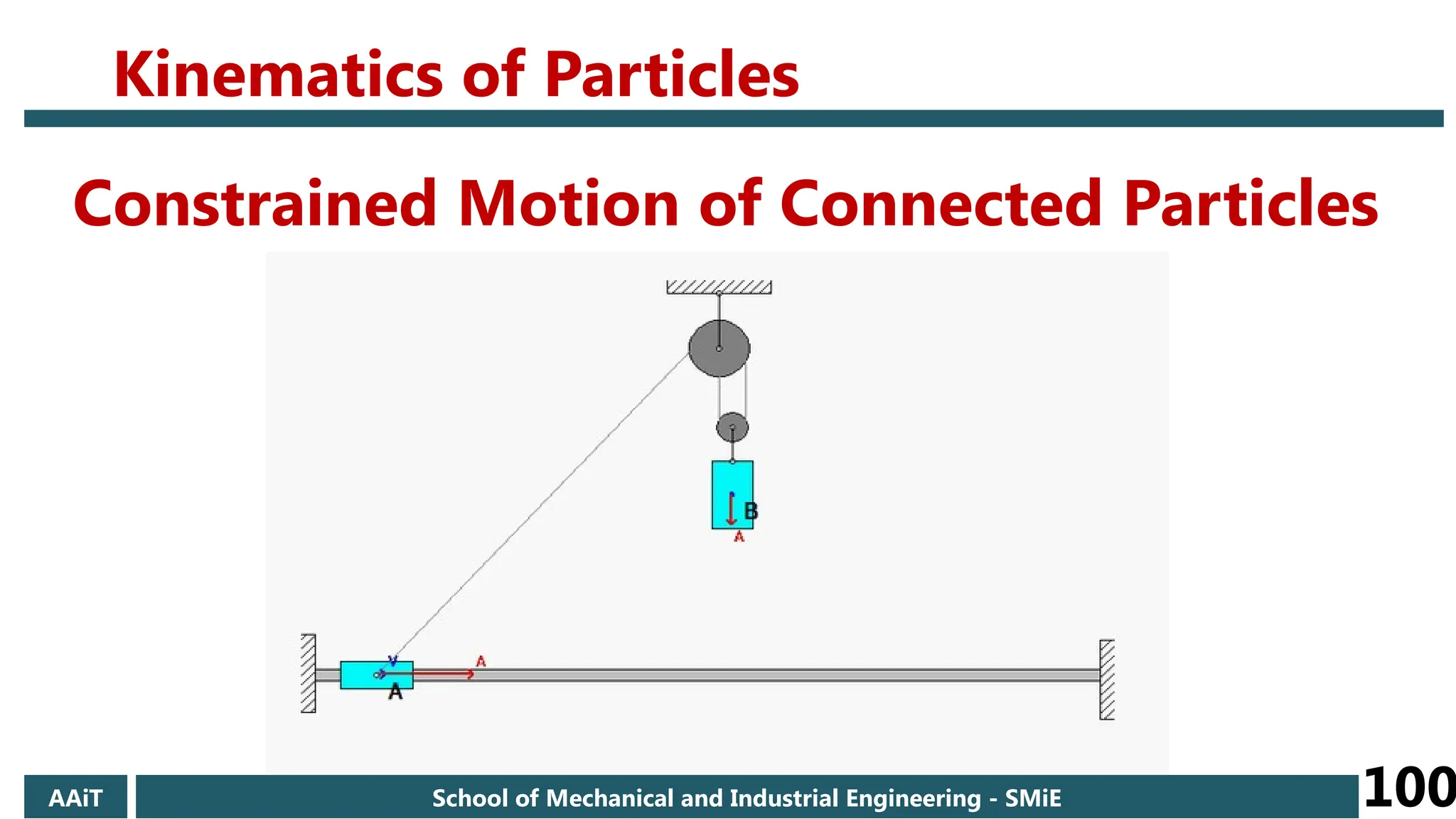
Constrained Motion of Connected Particles
Kinematics of Particles
101.
AAiT School ofMechanical and Industrial Engineering - SMiE 101
102.
Constrained Motion (DependentMotion)
• Sometimes the position of a particle will depend upon the
position of another or of several particles.
• If the particles are connected together by an inextensible ropes,
the resulting motion is called constrained motion
AAiT School of Mechanical and Industrial Engineering - SMiE 102
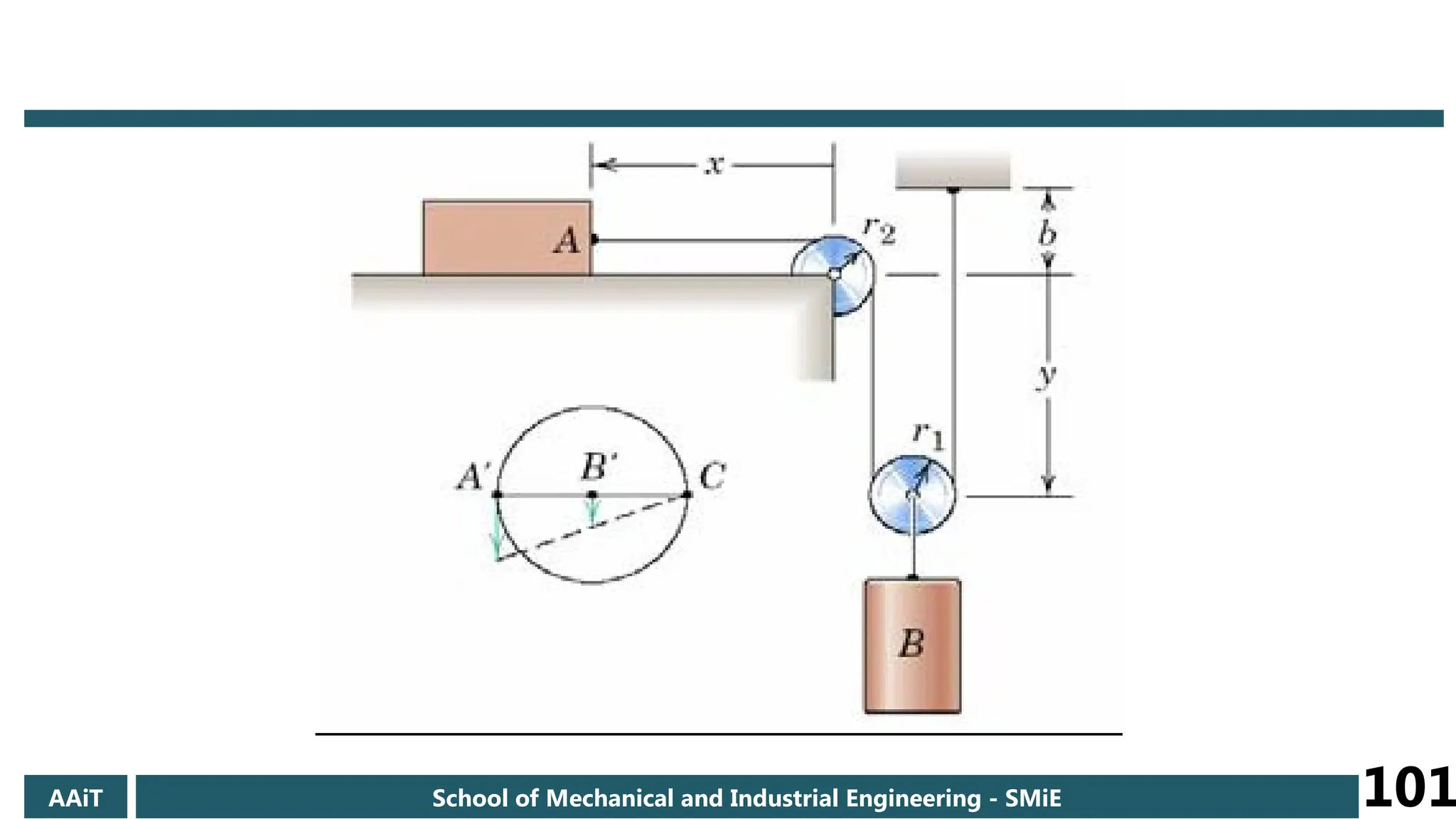
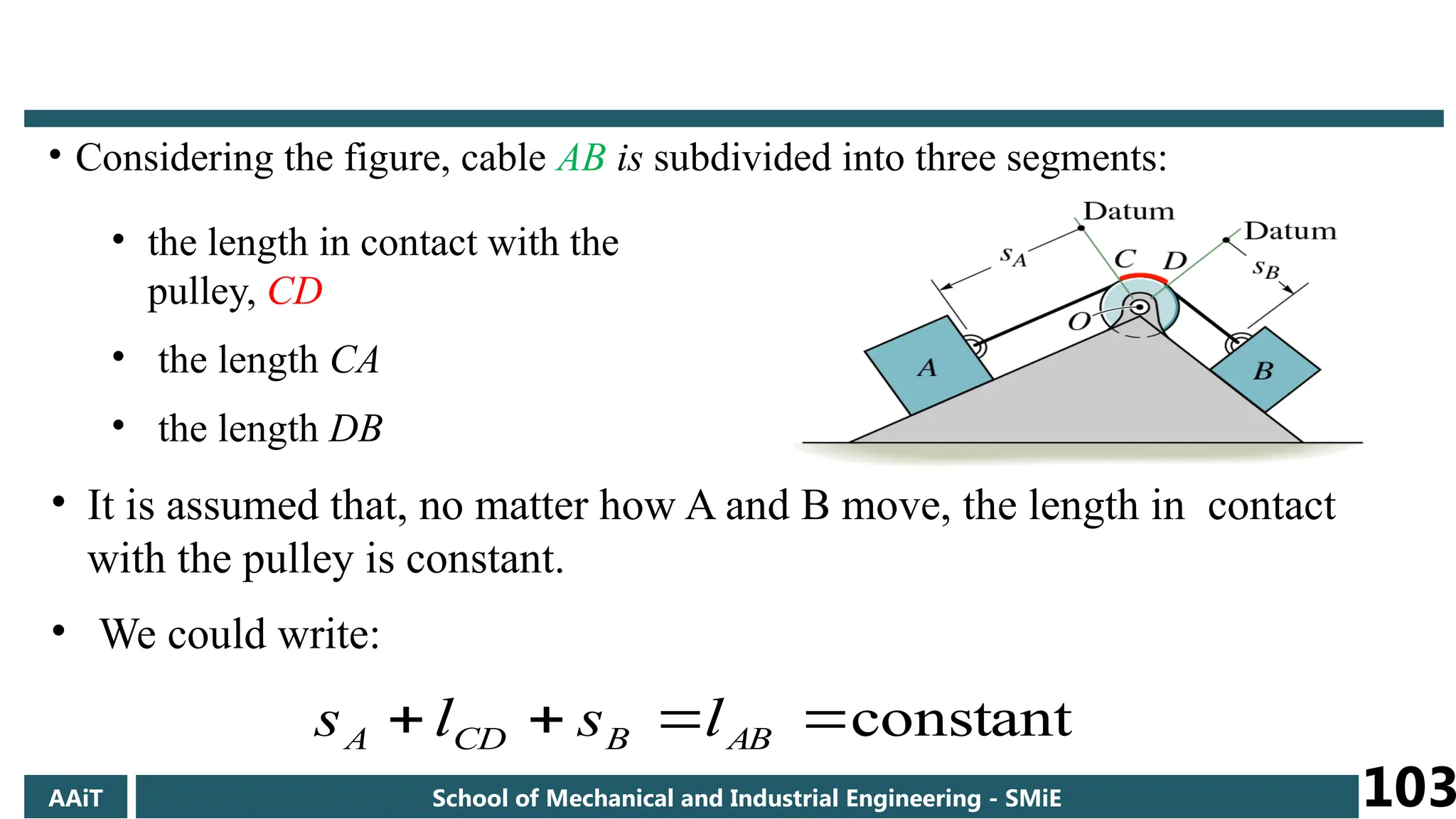
103.
• Considering thefigure, cable AB is subdivided into three segments:
• the length in contact with the
pulley, CD
• the length CA
• the length DB
• It is assumed that, no matter how A and B move, the length in contact
with the pulley is constant.
• We could write:
constant
AB
B
CD
A l
s
l
s
AAiT School of Mechanical and Industrial Engineering - SMiE 103
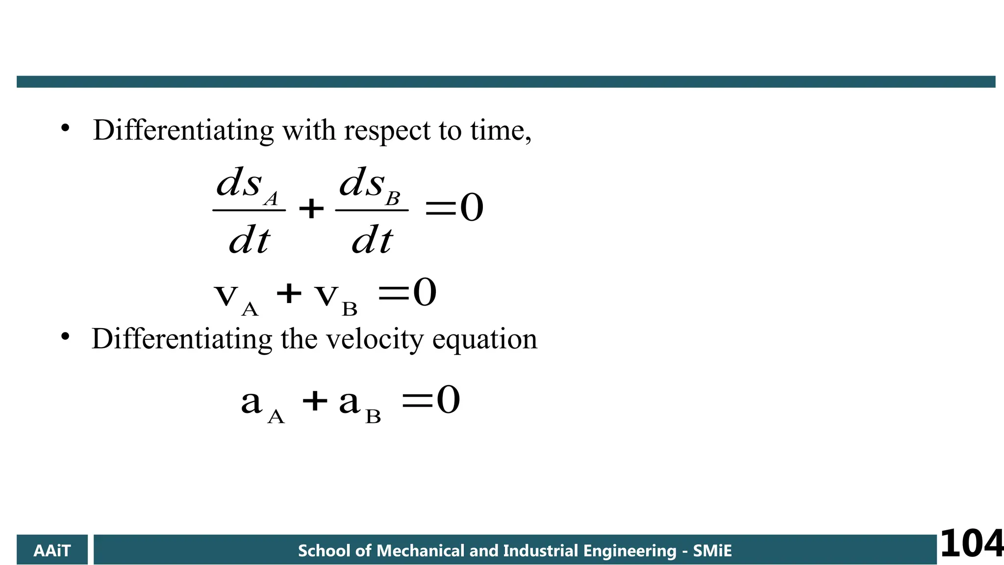
104.
• Differentiating withrespect to time,
• Differentiating the velocity equation
0
v
v
0
B
A
dt
ds
dt
ds B
A
0
a
a B
A
AAiT School of Mechanical and Industrial Engineering - SMiE 104
105.
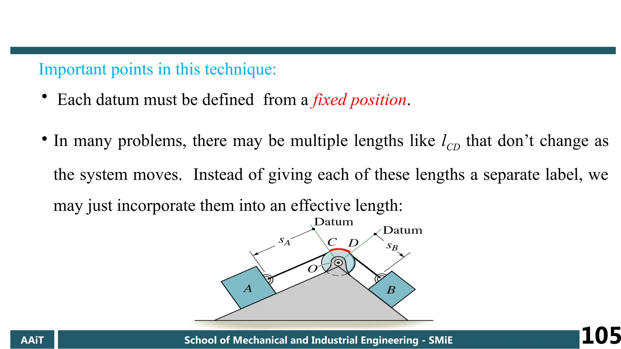
Important points inthis technique:
• Each datum must be defined from a fixed position.
• In many problems, there may be multiple lengths like lCD that don’t change as
the system moves. Instead of giving each of these lengths a separate label, we
may just incorporate them into an effective length:
AAiT School of Mechanical and Industrial Engineering - SMiE 105
106.
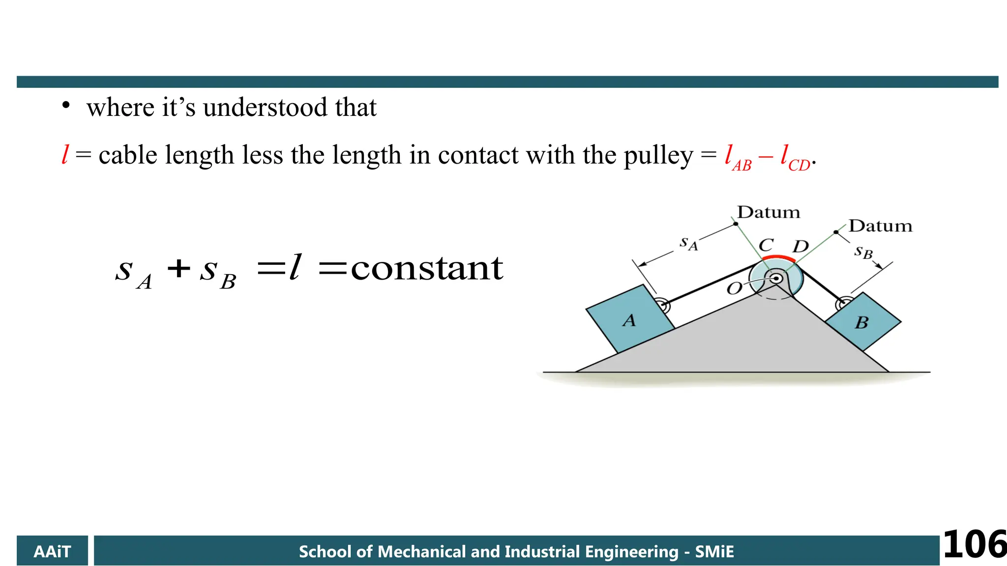
• where it’sunderstood that
l = cable length less the length in contact with the pulley = lAB – lCD.
constant
l
s
s B
A
AAiT School of Mechanical and Industrial Engineering - SMiE 106
107.
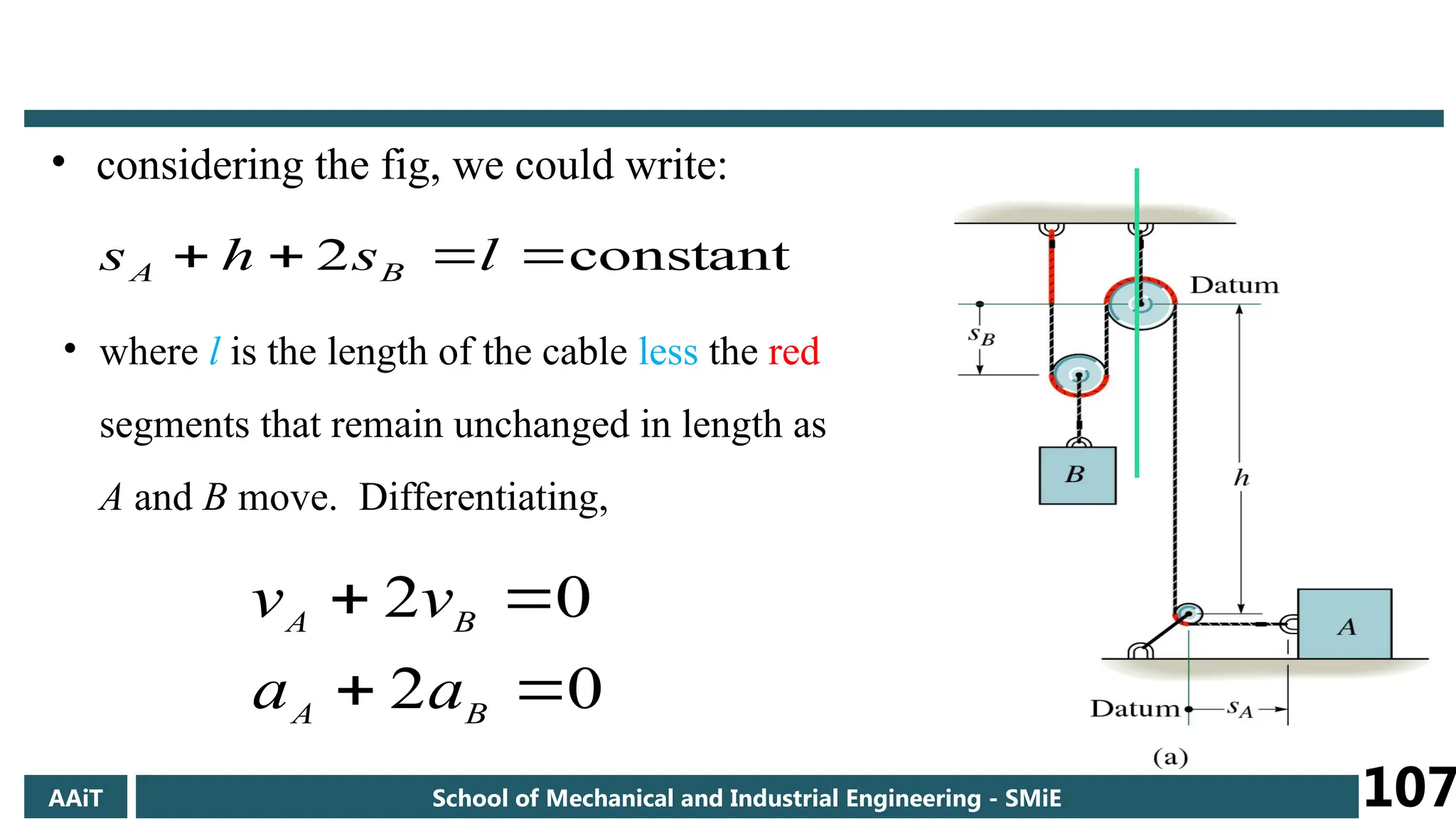
constant
2
l
s
h
sB
A
• considering the fig, we could write:
• where l is the length of the cable less the red
segments that remain unchanged in length as
A and B move. Differentiating,
0
2
0
2
B
A
B
A
a
a
v
v
AAiT School of Mechanical and Industrial Engineering - SMiE 107
108.
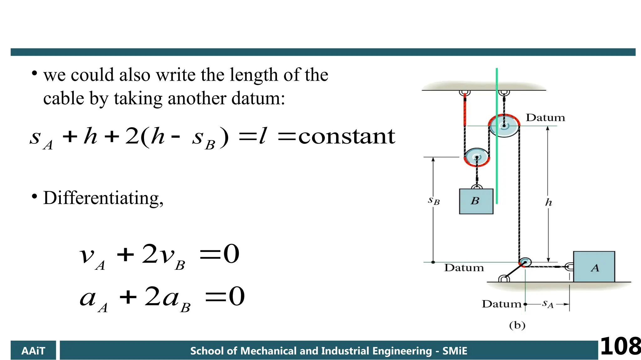
constant
)
(
2
l
s
h
h
sB
A
• we could also write the length of the
cable by taking another datum:
• Differentiating,
0
2
0
2
B
A
B
A
a
a
v
v
AAiT School of Mechanical and Industrial Engineering - SMiE 108
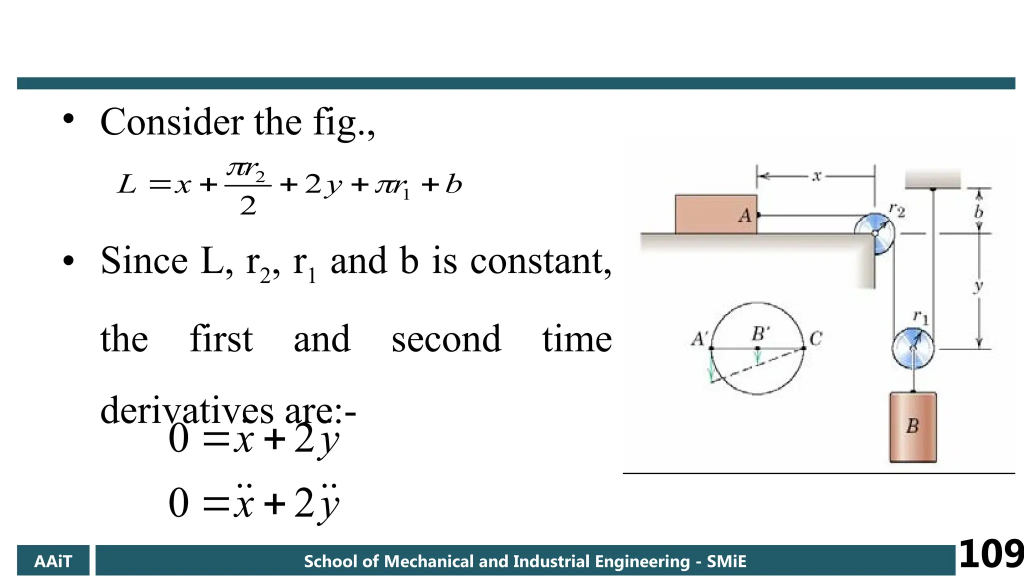
109.
• Consider thefig.,
• Since L, r2, r1 and b is constant,
the first and second time
derivatives are:-
b
r
y
r
x
L
1
2
2
2
y
x
y
x
2
0
2
0
AAiT School of Mechanical and Industrial Engineering - SMiE 109
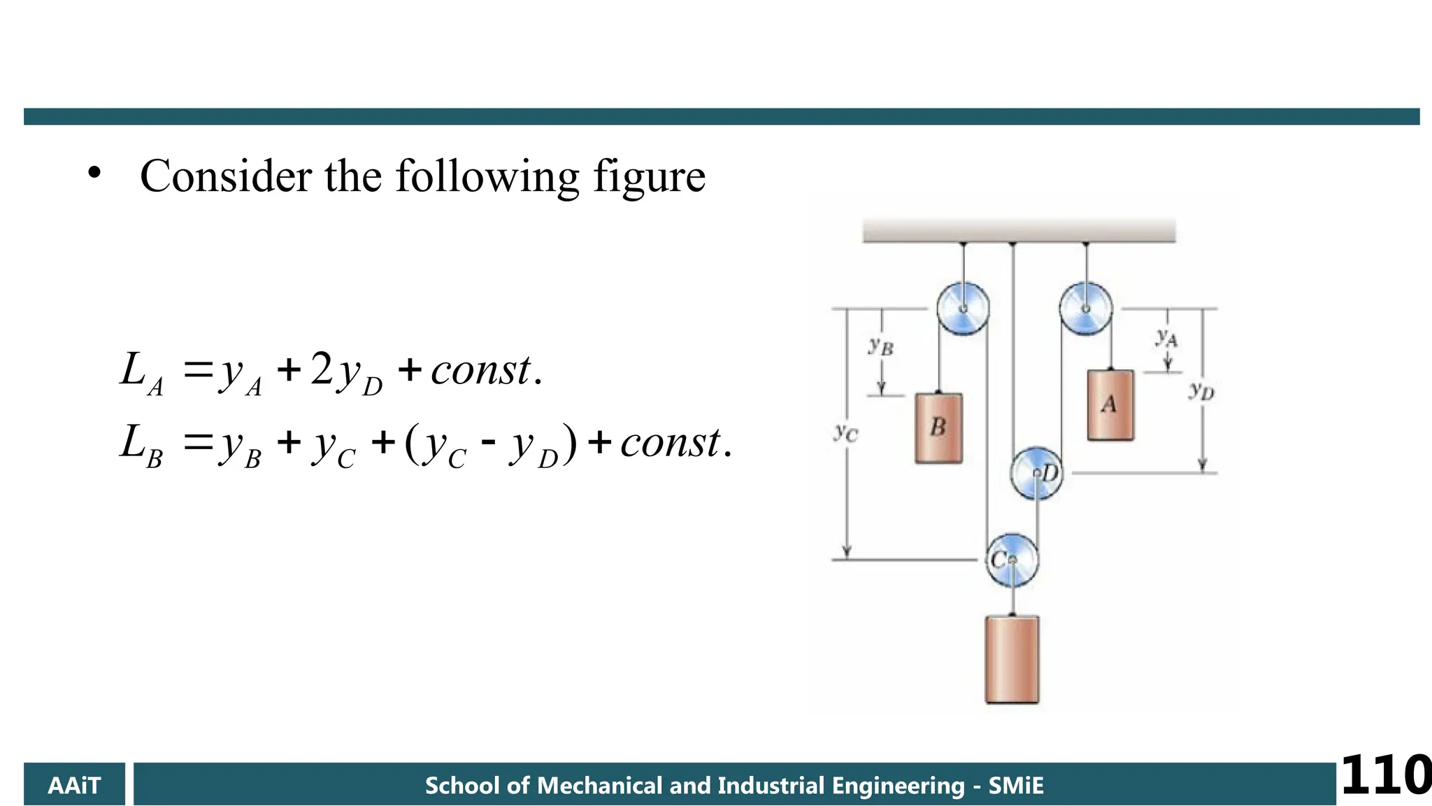
110.
• Consider thefollowing figure
.
)
(
.
2
const
y
y
y
y
L
const
y
y
L
D
C
C
B
B
D
A
A
AAiT School of Mechanical and Industrial Engineering - SMiE 110
111.
• NB. Clearly,it is impossible for the signs of all three
terms to be positive simultaneously.
AAiT School of Mechanical and Industrial Engineering - SMiE 111
112.
Suggested Problem
From 7th
Edition, Merriam
Engineering Mechanics Dynamics
Chapter II Problem 2/……..
58,48,22,18,44,43,62,79,76,85,81,83,93,
107,120,128,129,114,111,136,140,143,145,
161,154,152,118,220,221,214,189,199,204,
192, and 184
AAiT School of Mechanical and Industrial Engineering - SMiE 112