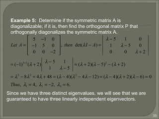
Downloaded 288 times


![16
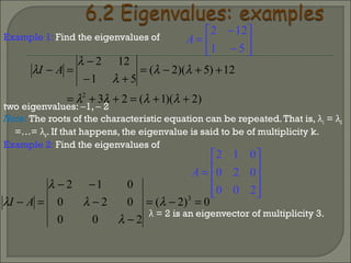
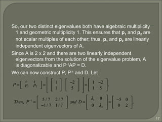
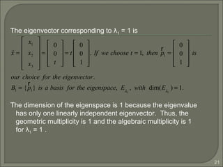
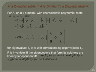
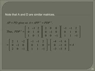
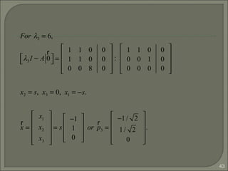
If P = [ p1 p2 ], then AP = PD even if A is not diagonalizable.
Since AP =
1 −2
1 5
−3 −2
−5 0
= A
r
p1
r
p2
= A
r
p1 A
r
p2
=
−5 −4
−5 10
=
−5(1) 2(−2)
−5(1) 2(5)
= −5
1
1
2
−2
5
= λ1
r
p1 λ2
r
p2
=
r
p1
r
p2
λ1 0
0 λ2
=
1
1
−2
5
−5 0
0 2
=
1 −2
1 5
−5 0
0 2
= PD.](https://image.slidesharecdn.com/eigenvaluesandeigenvectors-140622114942-phpapp01/85/Eigen-values-and-eigenvectors-16-320.jpg)
![33
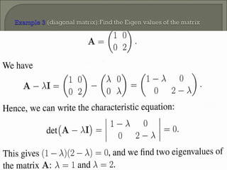
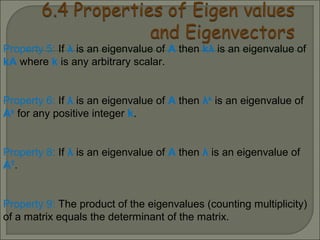
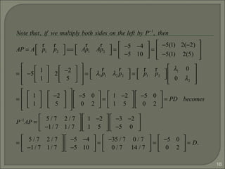
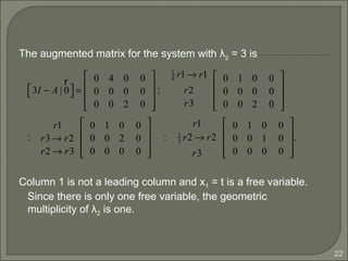
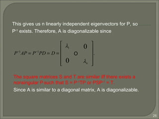
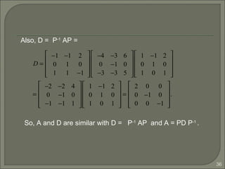
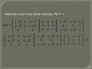
Thus, we have AP = PD as follows :
−4 −3 6
0 −1 0
−3 −3 5
1 −1 2
0 1 0
1 0 1
=
1 −1 2
0 1 0
1 0 1
2 0 0
0 −1 0
0 0 −1
2 1 −2
0 −1 0
2 0 −1
=
2 1 −2
0 −1 0
2 0 −1
.
Since the geometric multiplicity is equal to the algebraic
multiplicity for each distinct eigenvalue, we found three
linearly independent eigenvectors. The matrix A is
diagonalizable since P = [p1 p2 p3] is nonsingular.](https://image.slidesharecdn.com/eigenvaluesandeigenvectors-140622114942-phpapp01/85/Eigen-values-and-eigenvectors-33-320.jpg)
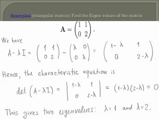
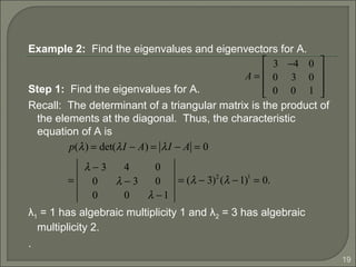
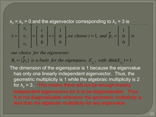
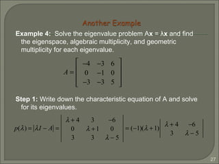
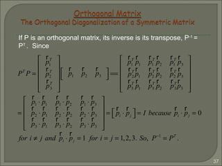
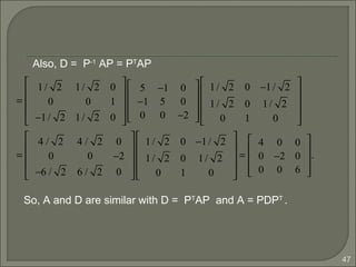
![34
P | I[ ]=
1 −1 2
0 1 0
1 0 1
1 0 0
0 1 0
0 0 1
:
1 −1 2
0 1 0
0 1 −1
1 0 0
0 1 0
−1 0 1
:
1 0 2
0 1 0
0 0 1
1 1 0
0 1 0
1 1 −1
:
1 0 0
0 1 0
0 0 1
−1 −1 2
0 1 0
1 1 −1
. So, P−1
=
−1 −1 2
0 1 0
1 1 −1
.
We can find P-1
as follows:](https://image.slidesharecdn.com/eigenvaluesandeigenvectors-140622114942-phpapp01/85/Eigen-values-and-eigenvectors-34-320.jpg)
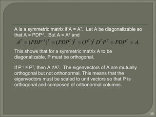
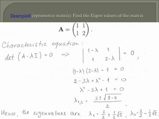
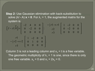
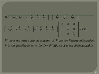
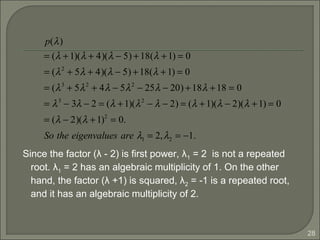
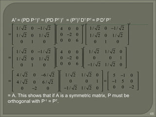
![44
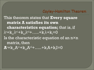
As we can see the eigenvectors of A are distinct, so {p1, p2,
p3} is linearly independent, P-1
exists for P =[p1 p2 p3] and
Thus A is diagonalizable.
Since A = AT
(A is a symmetric matrix) and P is orthogonal
with approximate scaling of p1, p2, p3, P-1
= PT
.
AP = PD ⇔ PDP−1
.
PP−1
= PPT
=
1/ 2 0 −1/ 2
1/ 2 0 1/ 2
0 1 0
1/ 2 1/ 2 0
0 0 1
−1/ 2 1/ 2 0
=
1 0 0
0 1 0
0 0 1
= I.](https://image.slidesharecdn.com/eigenvaluesandeigenvectors-140622114942-phpapp01/85/Eigen-values-and-eigenvectors-44-320.jpg)
![45
As we can see the eigenvectors of A are distinct, so {p1, p2,
p3} is linearly independent, P-1
exists for P =[p1 p2 p3] and
Thus A is diagonalizable.
Since A = AT
(A is a symmetric matrix) and P is orthogonal
with approximate scaling of p1, p2, p3, P-1
= PT
.
AP = PD ⇔ PDP−1
.
PP−1
= PPT
=
1/ 2 0 −1/ 2
1/ 2 0 1/ 2
0 1 0
1/ 2 1/ 2 0
0 0 1
−1/ 2 1/ 2 0
=
1 0 0
0 1 0
0 0 1
= I.](https://image.slidesharecdn.com/eigenvaluesandeigenvectors-140622114942-phpapp01/85/Eigen-values-and-eigenvectors-45-320.jpg)


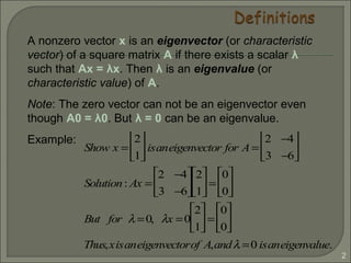
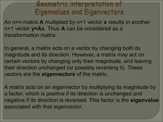
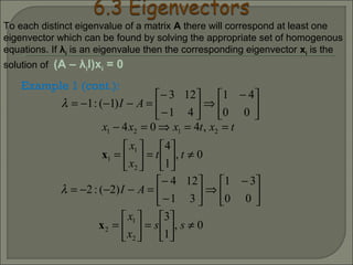
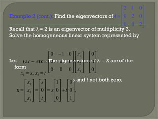
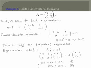
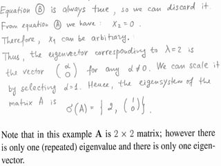
1) An eigenvector of a square matrix A is a non-zero vector x that satisfies the equation Ax = λx, where λ is the corresponding eigenvalue. 2) The zero vector cannot be an eigenvector, but λ = 0 can be an eigenvalue. 3) For a matrix A, the eigenvectors and eigenvalues can be found by solving the system of equations (A - λI)x = 0, where λI is the identity matrix multiplied by the eigenvalue λ.