Downloaded 39 times


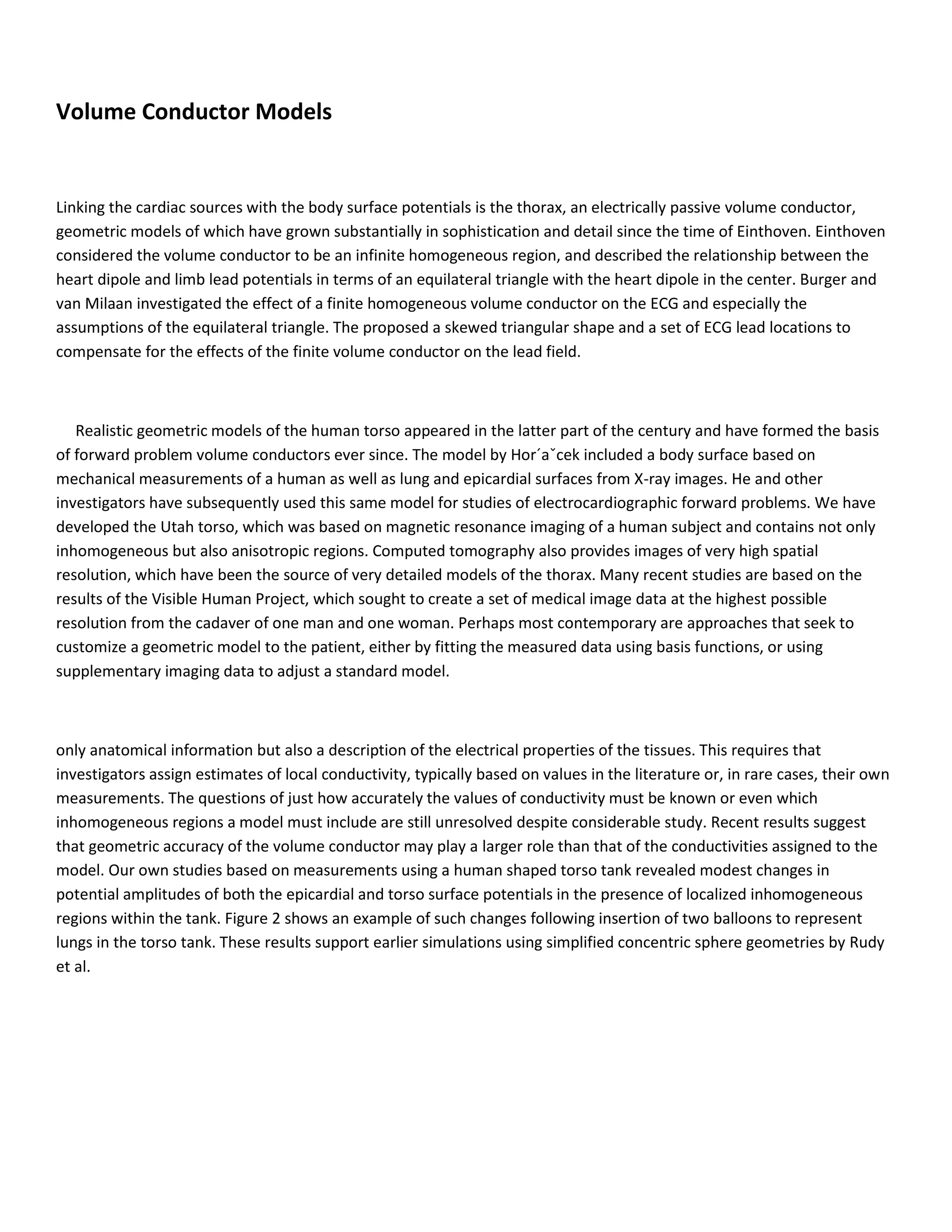
![is to relate the potentials recorded at the body surface with the
ones generated
on the heart surface as a result of the electrical activity of the
heart.
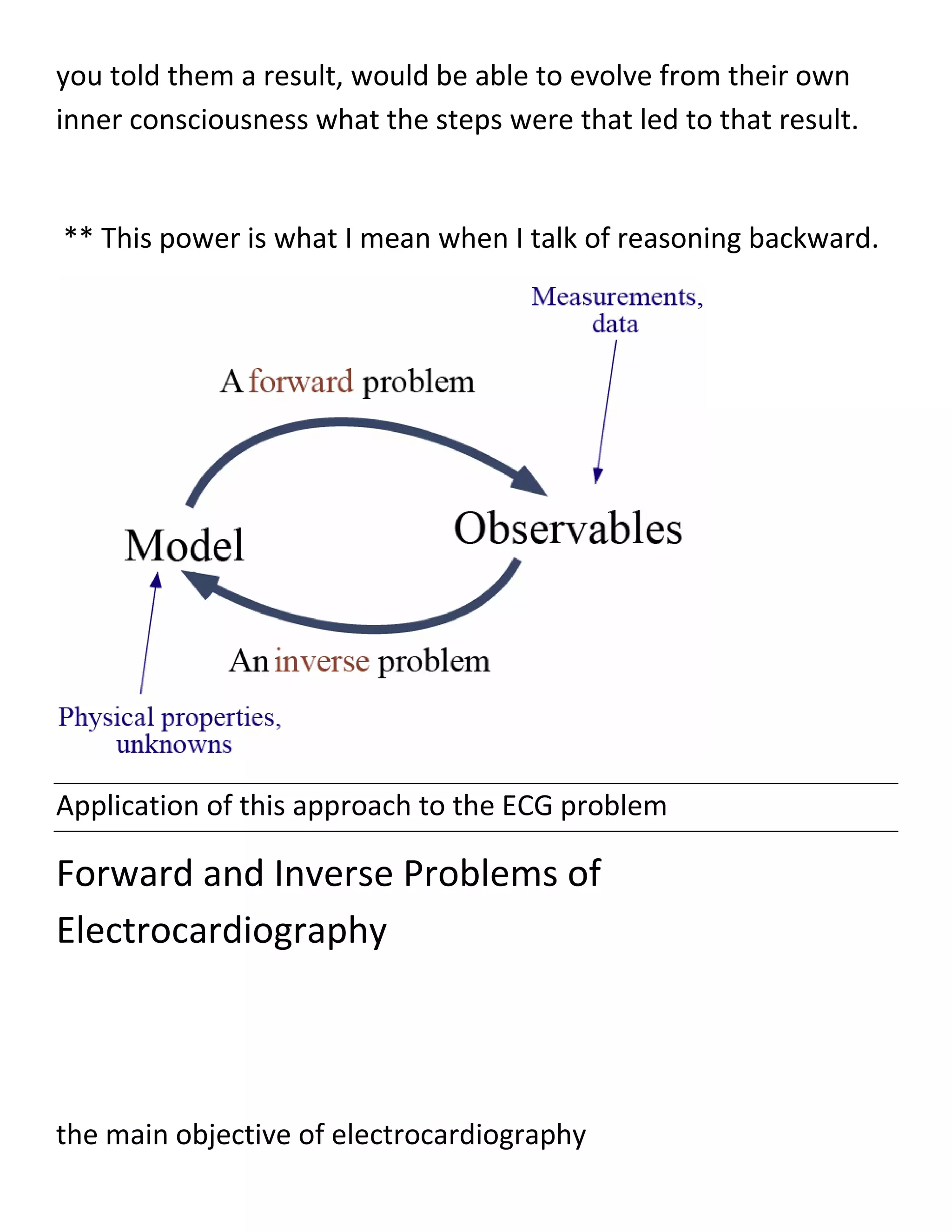
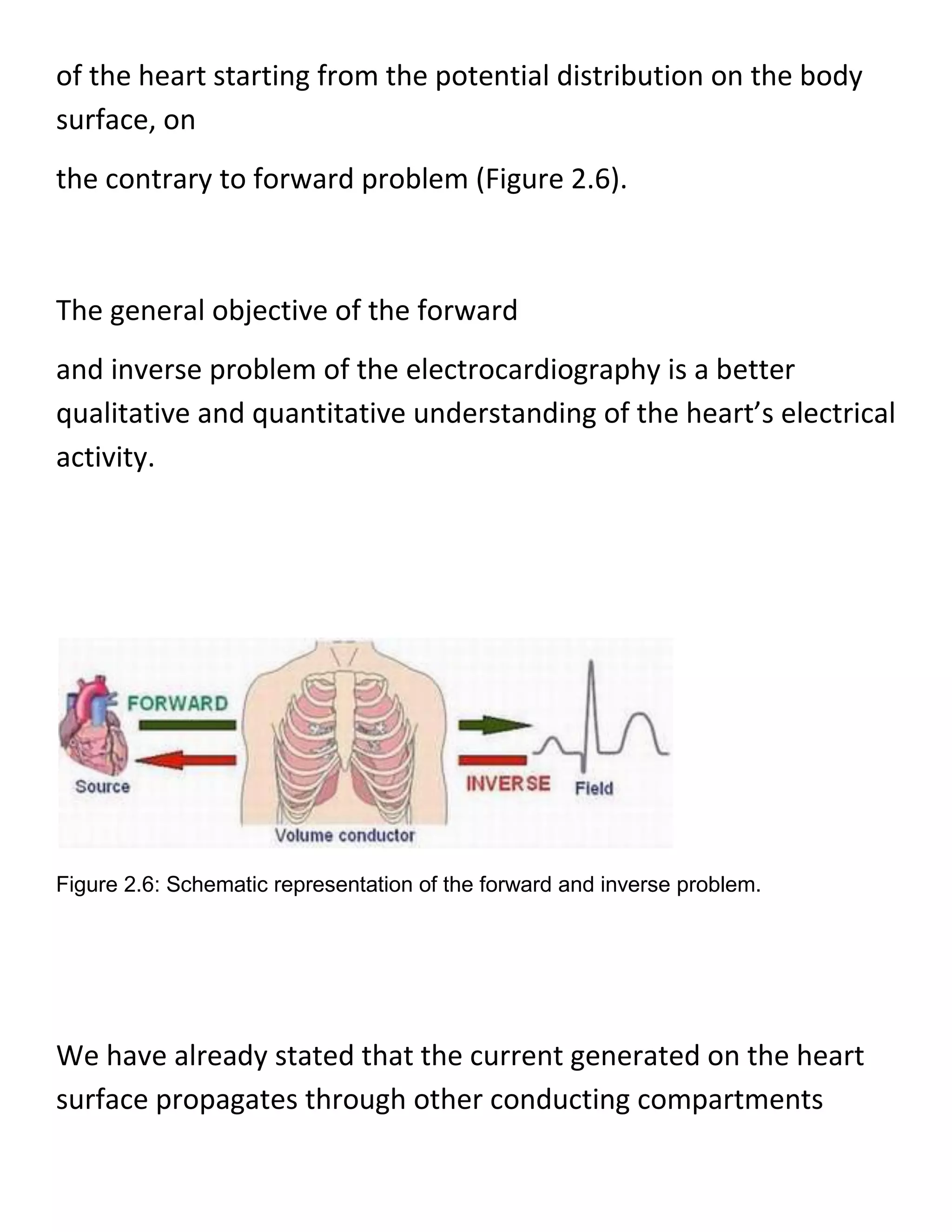
Two different approaches - in other words, problems — are used
in electrocardiography to establish this relation.
The first approach is called the forward
problem which entails the calculation of the body-surface
potentials, starting
usually from either pre-decided electrical representation of the
heart activity
(equivalent current dipoles) or from known potentials on the
heart’s surface
(the epicardium) [20].
The other approach is the inverse problem, which involves the
calculation of the potentials and prediction of the electrical
activity](https://image.slidesharecdn.com/247606d7-733d-4cc8-b631-063f4bd57645-150513232406-lva1-app6891/75/ECG-graduation-project-21-2048.jpg)
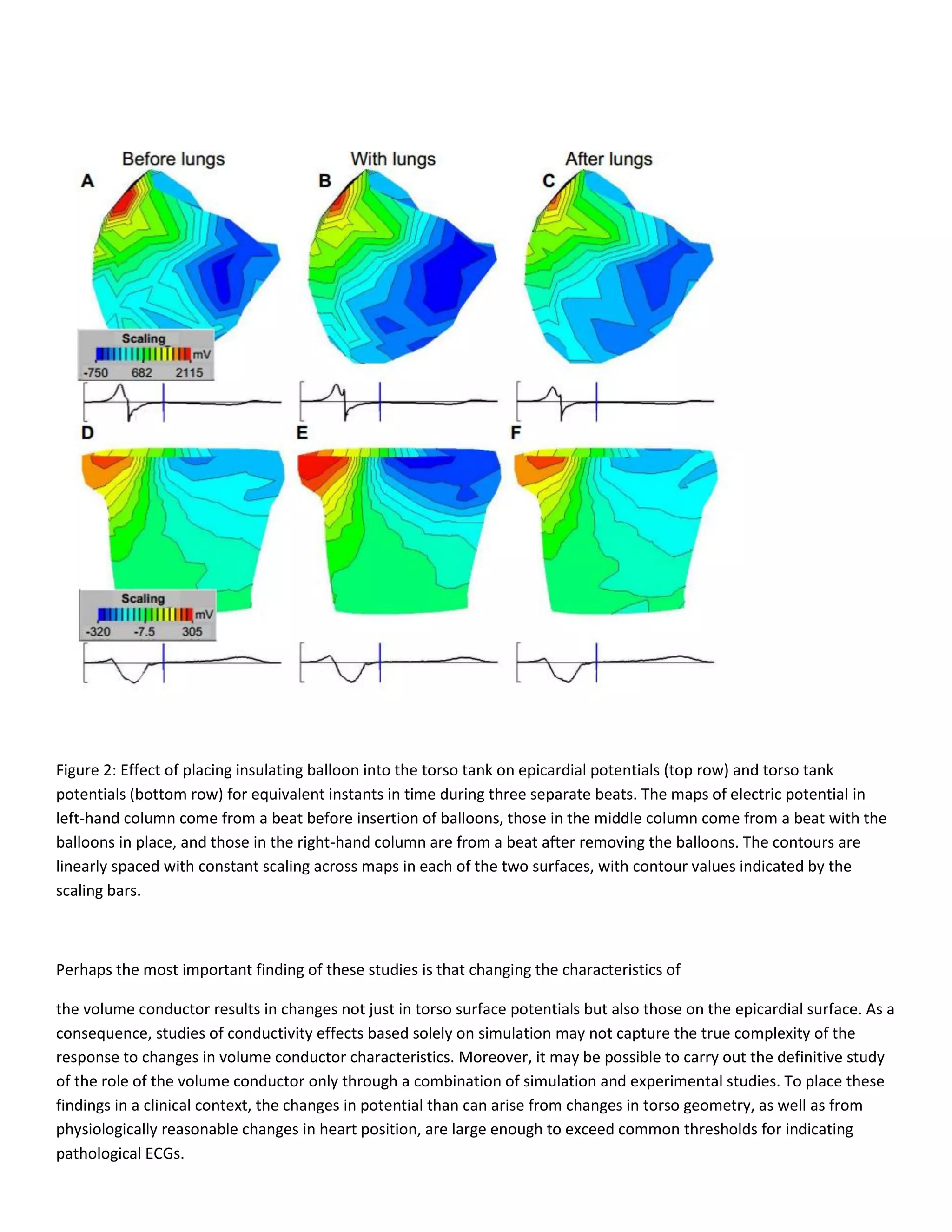
![For a specific solution to the forward or inverse solution of ECG, a
three dimensional geometric description of a volume conductor
(Figure 2.7) is required. The geometric description of
the volume conductor can take several forms, depending on the
specific method
of mathematical solution [9.]
When considering a realistic torso as in Figure 2.7, we have
several regions
which are physically different and have different electrical
conductivities.
This means that the volume conductor is inhomogeneous.
Sometimes, in order to simplify the calculations, the conducting
medium between the heart and body surface, inside of the torso,
is assumed to be similar in geometry and have the same
conductivity values.
In that case, the torso is described as homogeneous.](https://image.slidesharecdn.com/247606d7-733d-4cc8-b631-063f4bd57645-150513232406-lva1-app6891/75/ECG-graduation-project-24-2048.jpg)
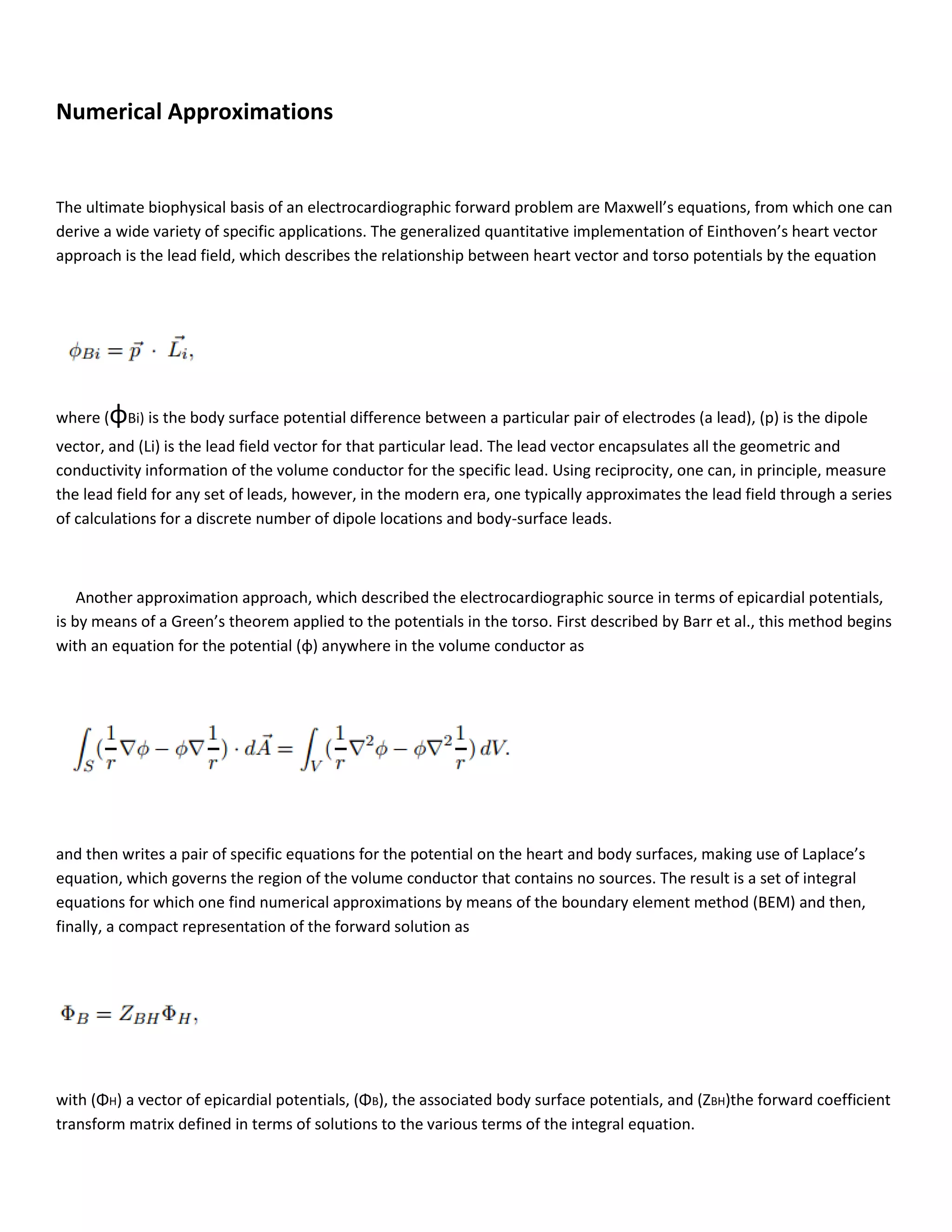
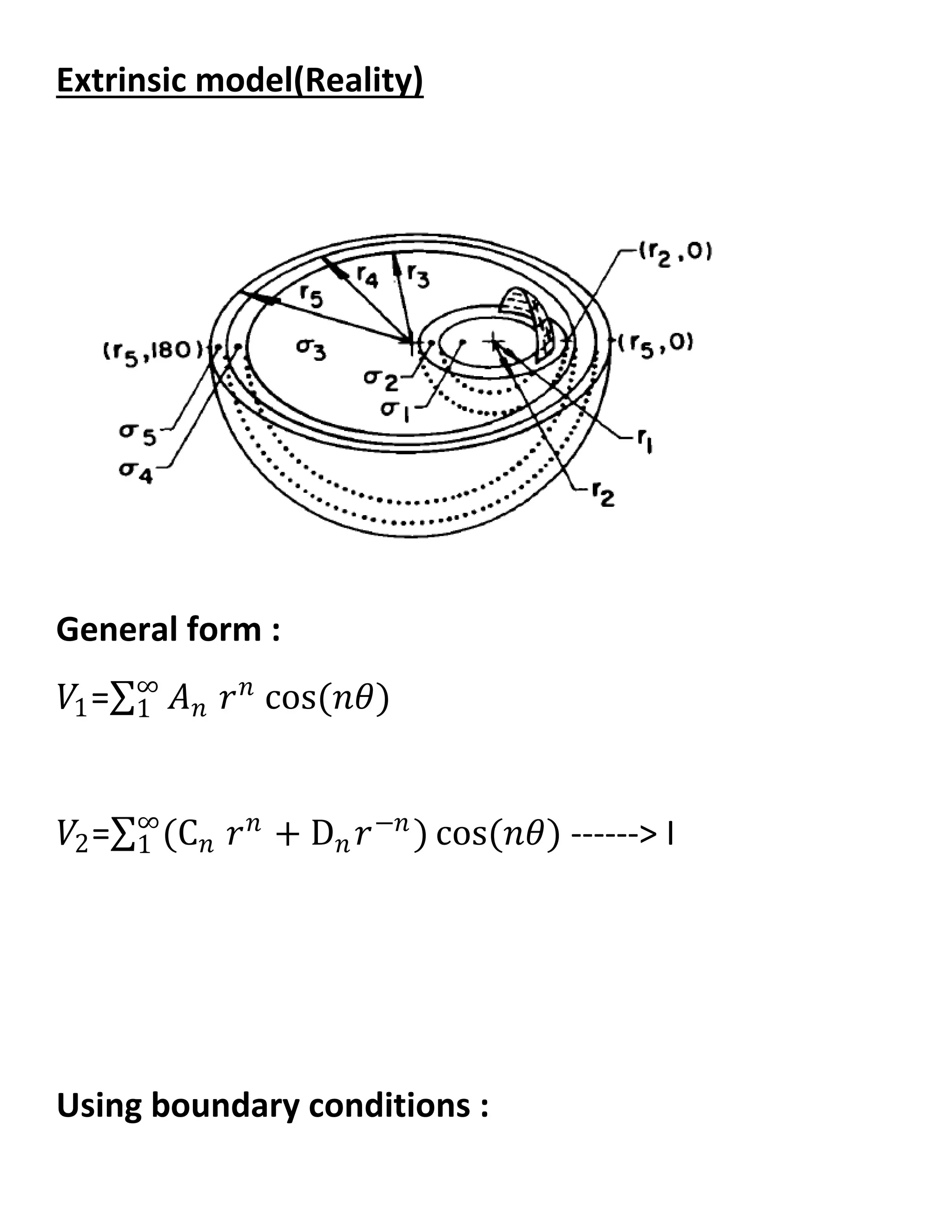
![Figure 2.7: Geometric description of the volume conductor.
Moreover, if the conductivity value in a region changes with the
direction then the region is defined to be anisotropic, otherwise, if
the conductivity is constant ver the region then the region is
isotropic.
One of the key differences between the forward and inverse
problems is that the forward solutions are generally unique; on
the other hand, the inverse
solutions are generally not unique [9].](https://image.slidesharecdn.com/247606d7-733d-4cc8-b631-063f4bd57645-150513232406-lva1-app6891/75/ECG-graduation-project-25-2048.jpg)
![Being not unique arises from the reason
that the primary cardiac sources cannot be uniquely determined
as long as the active cardiac region containing these sources is
inaccessible for potential easurements.
This is because the electric field that these sources generate
outside any closed surface completely enclosing them may be
duplicated by
equivalent single-layer (monopole) or double-layer (dipole)
current sources on he closed surface itself.
Many equivalent sources and, hence, inverse solutions,are thus
possible. However, once an equivalent source (and associated
volume
conductor) is selected, its parameters can usually be determined
uniquely from
the body-surface potentials [20.]
One drawback of the inverse problems is that, computationally,
inverse problems frequently involve complex numerical
algorithms and large systems of equations.](https://image.slidesharecdn.com/247606d7-733d-4cc8-b631-063f4bd57645-150513232406-lva1-app6891/75/ECG-graduation-project-26-2048.jpg)
![In addition, inverse problems are also typically ill-posed, that is,
small changes in the input data can lead to deviations in the
solutions.
Often, the ajor challenge of an inverse problem lies in
incorporating a priori information
into the solution by regularizations and improvements [25].
The SCI Institute has developed a number of efficient and realistic
ways to solve a wide variety
of inverse problems in functional imaging - including
reconstruction of electrical
sources within the heart or brain and extraction of molecular
diffusion
information from magnetic resonance images [31.]
The content of this study does not include the inverse problem,
but the
forward problem of ECG.](https://image.slidesharecdn.com/247606d7-733d-4cc8-b631-063f4bd57645-150513232406-lva1-app6891/75/ECG-graduation-project-27-2048.jpg)
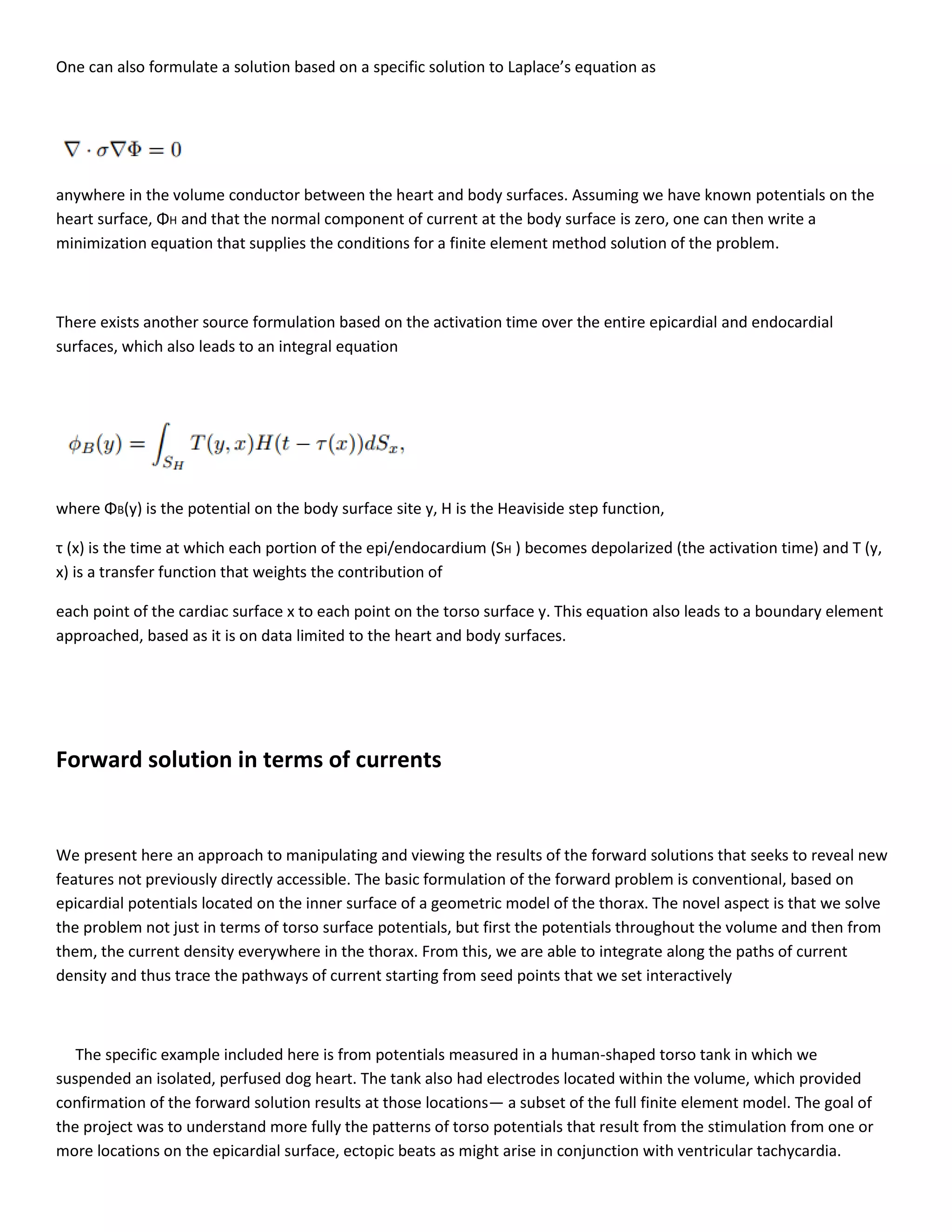
![The above information has been given to make clear the two
problems of ECG and relations, however, one can find a discussion
on
inverse problems in A.5
Forward Simulation
In the present study the left ventricle is subdivided into 17
segments (see Fig. 3b and 3c) according
to the recommendation from the American Heart Association (see
Fig. 3a) [Cerqueira MD et al., 2002;
Keller DUJ et al., 2006.]](https://image.slidesharecdn.com/247606d7-733d-4cc8-b631-063f4bd57645-150513232406-lva1-app6891/75/ECG-graduation-project-28-2048.jpg)
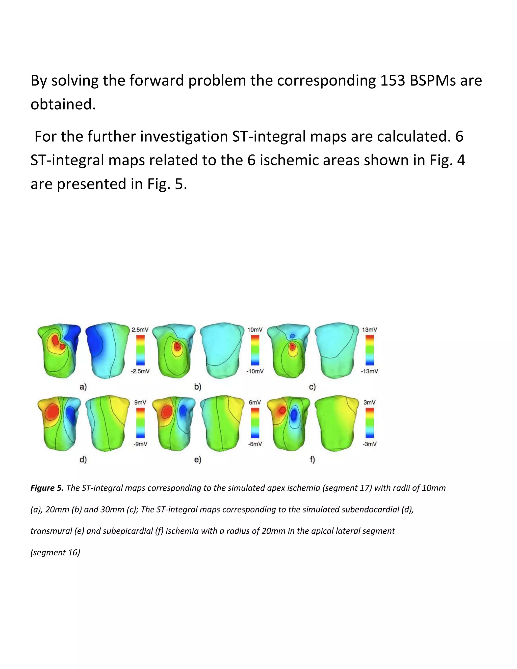
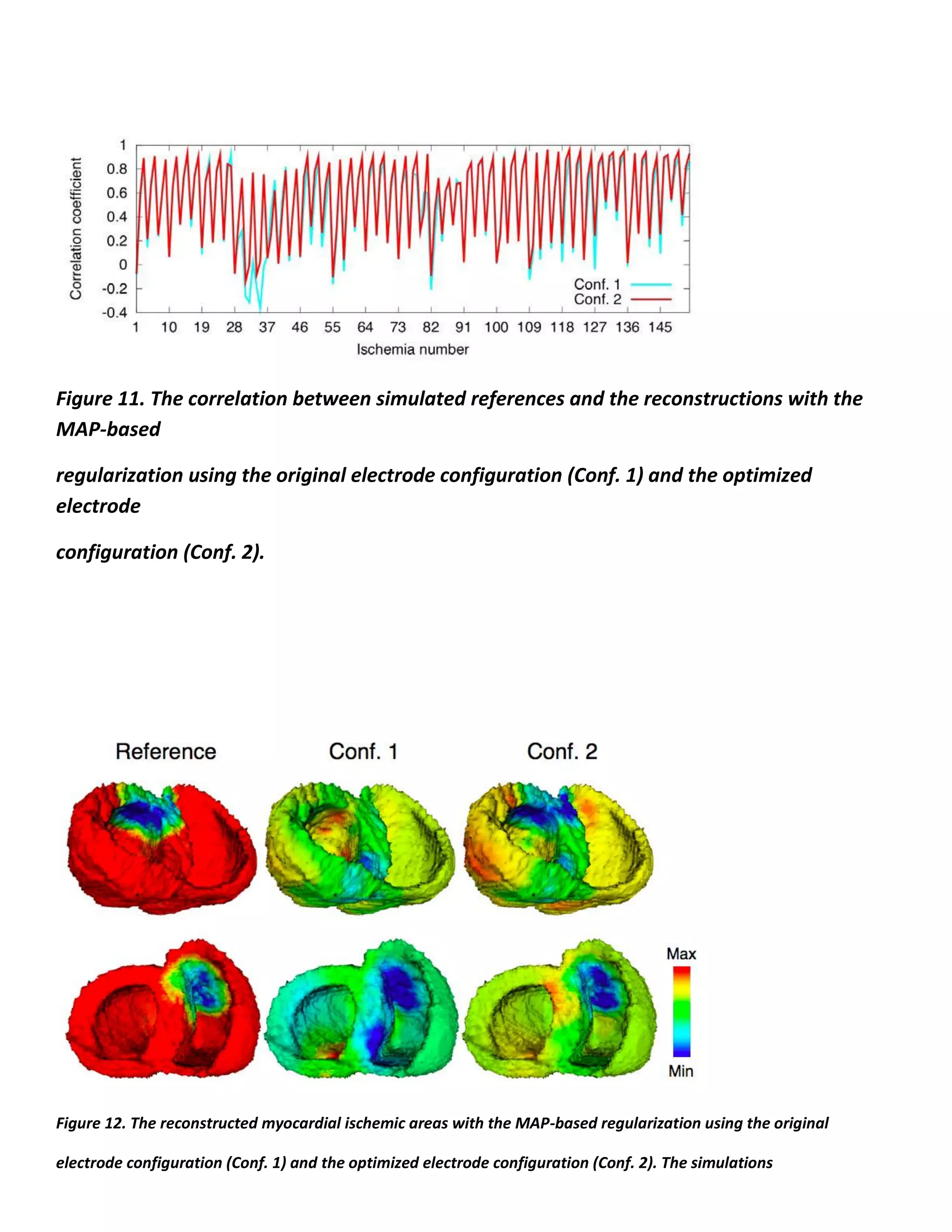
![Figure 3. The nomenclature of 17 AHA segments in left ventricle
[Cerqueira MD et al., 2002] (a) and the
subdivision of the left ventricular model according to the AHA suggestion
shown in two aspects (b) (c)
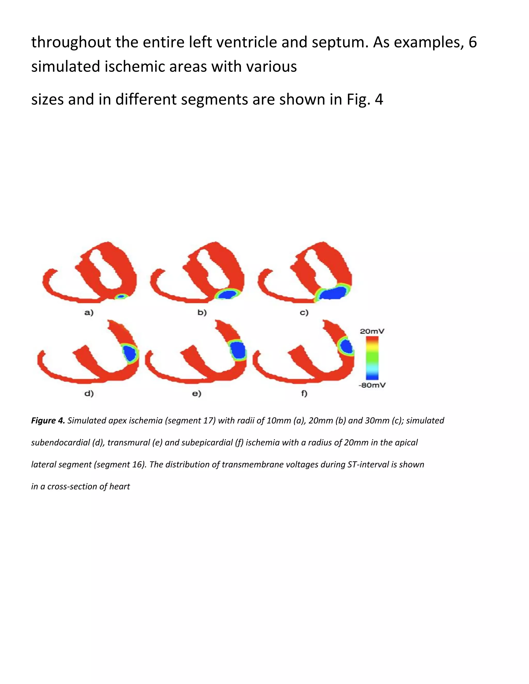
In each segment 3 types of ischemia are simulated, i.e.,
subendocardial, transmural and
subepicardial ischemia. For each type, 3 different sizes are
considered, i.e., 10mm, 20mm and 30mm
for the radius of ischemic area.
Thus, in total 153 different myocardial ischemic areas are
simulated](https://image.slidesharecdn.com/247606d7-733d-4cc8-b631-063f4bd57645-150513232406-lva1-app6891/75/ECG-graduation-project-29-2048.jpg)


![theta1=[(-pi):(pi/300):(pi)];
%equation of the source m(theta)
s=0;
for n=1:100;
m1=(1/6)*cos(n*theta1)*(sin(n*(pi/6)))/(n*pi/6);
s=s+m1;
end
m1=s+(1/6);
figure
plot(theta1,m1)
title('thetan1=pi/3 & m(theta) & n=1:100')
Output figure for m(theta) :
Matlab code for m(f) :
thetan1=pi/3;
theta1=[(-pi/6):(pi/300):(pi/6)];
%equation of the source m(theta)
s=0;
for n=1:100;
m1=(1/6)*cos(n*theta1)*(sin(n*(pi/6)))/(n*pi/6);
s=s+m1;
end
m1=s+(1/6);
mf=-fftshift(m1);
owmega=linspace(-10,10,length(mf));
figure
plot(owmega,mf)
title('owmega & m(f)')](https://image.slidesharecdn.com/247606d7-733d-4cc8-b631-063f4bd57645-150513232406-lva1-app6891/75/ECG-graduation-project-54-2048.jpg)
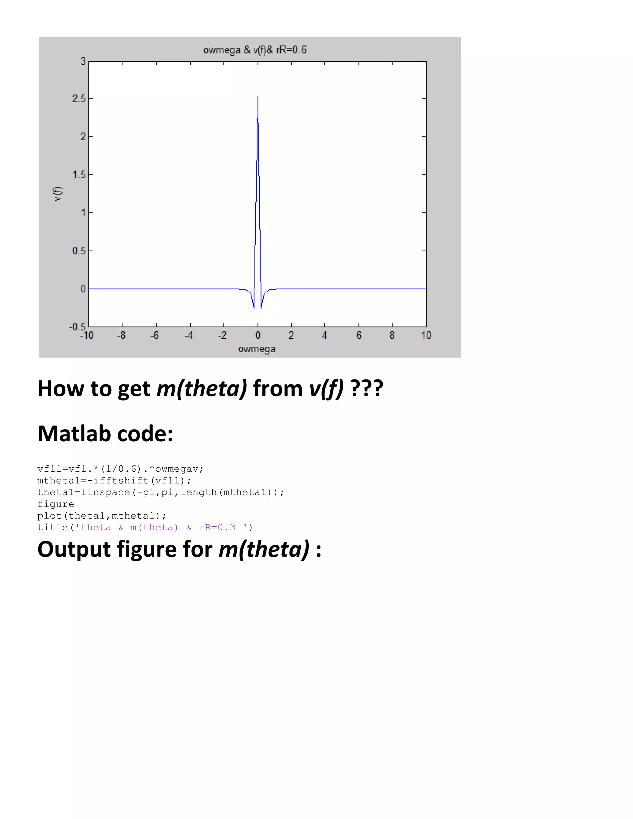
![Output figure for m(f) :
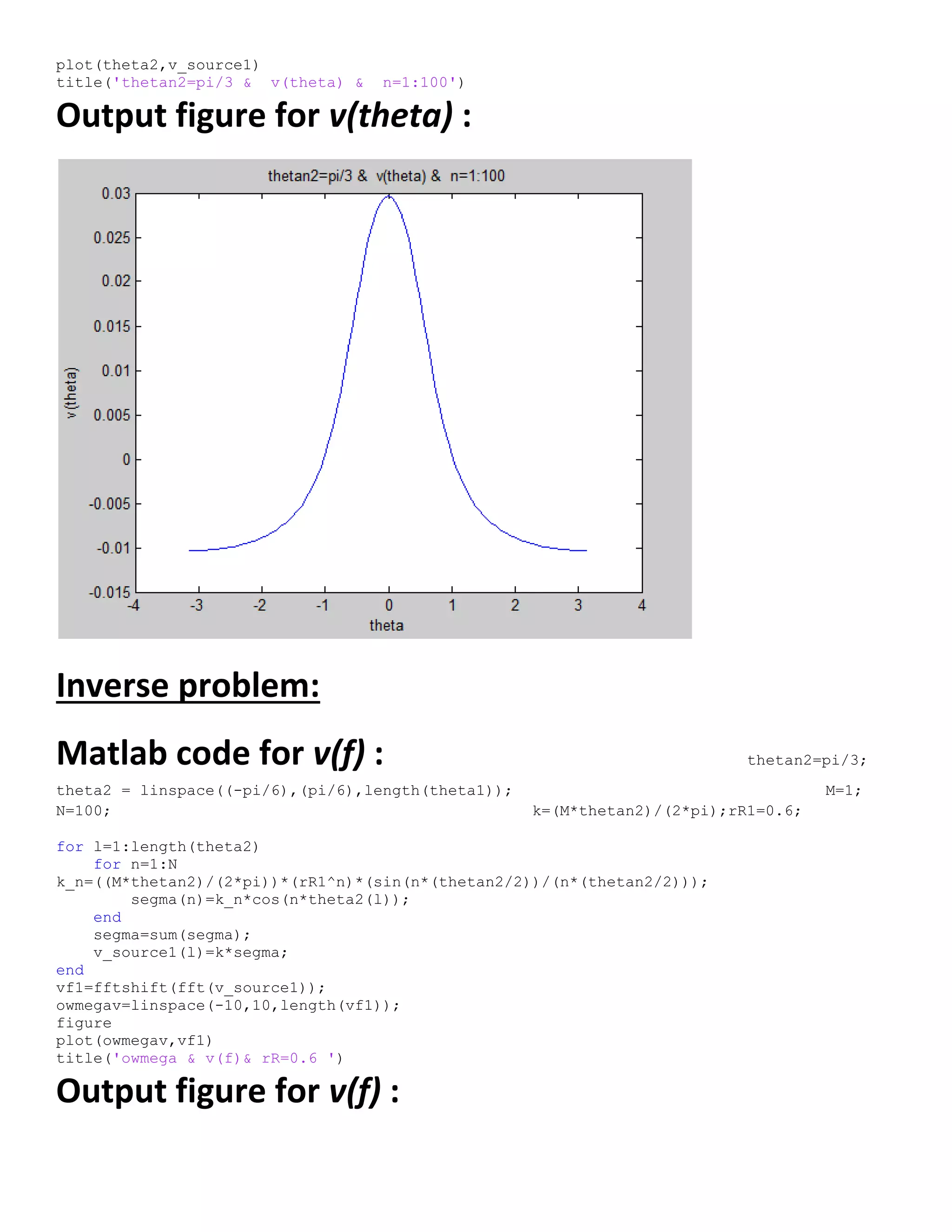
Matlab code for v(theta) :
%equation to get volt on the source
%theta2=[-pi:.001:pi];
thetan2=pi/3;
theta2 = linspace((-pi),(pi),length(theta1));
M=1;
N=100; % index of summation
k=(M*thetan2)/(2*pi);
rR1=0.6;
% loop to get surface voltage as a function of theta
%-----------------------------------------------------------
for l=1:length(theta2)
for n=1:N
k_n=((M*thetan2)/(2*pi))*(rR1^n)*(sin(n*(thetan2/2))/(n*(thetan2/2)));
segma(n)=k_n*cos(n*theta2(l));
end
segma=sum(segma);
v_source1(l)=k*segma;
end
figure](https://image.slidesharecdn.com/247606d7-733d-4cc8-b631-063f4bd57645-150513232406-lva1-app6891/75/ECG-graduation-project-55-2048.jpg)

![𝜕𝑉1
𝜕𝑟
= 𝑛𝐴 𝑛 𝑟 𝑛−1
cos(𝑛𝜃)
𝜕𝑉2
𝜕𝑟
= (𝑛C 𝑛 𝑟 𝑛−1 − 𝑛𝐷𝑛 𝑟−𝑛−1) cos(𝑛𝜃) ----->II
@r=𝑟°
𝜕𝑉1
𝜕𝑟
|𝑟° =
𝜕𝑉2
𝜕𝑟
|𝑟°
𝑛𝐴 𝑛 𝑟 𝑛−1 = 𝑛C 𝑛 𝑟 𝑛−1 − 𝑛𝐷𝑛 𝑟−𝑛−1
𝐷𝑛 = (C 𝑛 − A 𝑛)𝑟°
2𝑛
------> (1)
𝑉2 − 𝑉1|𝑟° = m(𝜃)
𝑉2 − 𝑉1|𝑟° =
𝑀𝜃°
2𝜋
+
𝑀𝜃°
2
sin (
𝑛𝜃
2
)
(
𝑛𝜃
2
)
cos(𝑛𝜃) ∞
1 --->(2)
𝑉2 − 𝑉1|𝑟° = [(C 𝑛 𝑟°
𝑛
+ D 𝑛 𝑟°
−𝑛
) − 𝐴 𝑛 𝑟°
𝑛
] cos(𝑛𝜃)∞
1 …(3)
From equ(2) , equ(3) :
𝑀𝜃°
2
sin (
𝑛𝜃
2
)
(
𝑛𝜃
2
)
cos(𝑛𝜃) = (C 𝑛 𝑟°
𝑛
+ D 𝑛 𝑟°
−𝑛
) − 𝐴 𝑛 𝑟°
𝑛
…..(4)
From equ(1):
𝐷 𝑛
𝑟°
2𝑛 = C 𝑛 − A 𝑛 ……..(5)](https://image.slidesharecdn.com/247606d7-733d-4cc8-b631-063f4bd57645-150513232406-lva1-app6891/75/ECG-graduation-project-60-2048.jpg)

![𝜕 𝑉2
𝜕𝑟′ = (𝑛C 𝑛 𝑟′ 𝑛−1
− 𝑛𝐷𝑛 𝑟′ −𝑛−1
) cos 𝑛𝜃 [ cos(𝜃).(
r
𝑟′
cos(𝜃) +
𝑥°
𝑟′
) + sin(𝜃)(
r
𝑟′
sin(𝜃) +
𝑦°
𝑟′
) ]
- (C 𝑛 𝑟′ 𝑛
+ D 𝑛 𝑟′ −𝑛
)[ sin 𝑛𝜃 (sin(𝜃) (
r
𝑟′
cos(𝜃) +
𝑥°
𝑟′
) - cos(𝜃)(
r
𝑟′
sin(𝜃) +
𝑦°
𝑟′
) ]
𝜕 𝑉2
𝜕𝑟′ = 𝑛C 𝑛 𝑟′ 𝑛−1
cos 𝑛𝜃 [ cos(𝜃).(
r
𝑟′
cos(𝜃) +
𝑥°
𝑟′
) + sin(𝜃)(
r
𝑟′
sin(𝜃) +
𝑦°
𝑟′
) ]
−𝑛𝐷𝑛 𝑟′ −𝑛−1
cos 𝑛𝜃 [ cos(𝜃).(
r
𝑟′
cos(𝜃) +
𝑥°
𝑟′
) + sin(𝜃)(
r
𝑟′
sin(𝜃) +
𝑦°
𝑟′
) ]
−𝑛C 𝑛 𝑟′ 𝑛−1
sin(𝑛𝜃)[
𝑥°
𝑟′
sin(𝜃) −
𝑦°
𝑟′
cos(𝜃) ]
−𝑛𝐷𝑛 𝑟′ −𝑛−1
sin(𝑛𝜃)[
𝑥°
𝑟′
sin(𝜃) −
𝑦°
𝑟′
cos(𝜃) ]
𝜕 𝑉2
𝜕𝑟′ = 𝑛C 𝑛 𝑟′ 𝑛−1
[ cos 𝑛𝜃 (
r
𝑟′
𝑐𝑜𝑠2
(𝜃) +
𝑥°
𝑟′
cos(𝜃) +
r
𝑟′
𝑠𝑖𝑛2
(𝜃) +
𝑦°
𝑟′
sin(𝜃) )− sin(𝑛𝜃)(
𝑥°
𝑟′
sin(𝜃) −
𝑦°
𝑟′
cos(𝜃) ) ]
−𝑛𝐷𝑛 𝑟′ −𝑛−1
[ cos 𝑛𝜃 (
r
𝑟′
𝑐𝑜𝑠2
(𝜃) +
𝑥°
𝑟′
cos(𝜃) +
r
𝑟′
𝑠𝑖𝑛2
(𝜃) +
𝑦°
𝑟′
sin(𝜃) )+ sin(𝑛𝜃)(
𝑥°
𝑟′
sin(𝜃) −
𝑦°
𝑟′
cos(𝜃) ) ]
@
𝜕 𝑉2
𝜕𝑟′ |R = 0
[
R2𝑛 Cn −Dn
Dn
][ cos 𝑛𝜃 (
r
R
𝑐𝑜𝑠2
𝜃 +
𝑥°
R
cos 𝜃 +
r
R
𝑠𝑖𝑛2
𝜃 +
𝑦°
R
sin 𝜃](https://image.slidesharecdn.com/247606d7-733d-4cc8-b631-063f4bd57645-150513232406-lva1-app6891/75/ECG-graduation-project-64-2048.jpg)
![− [
R2𝑛 Cn −Dn
Dn
][ sin(𝑛𝜃)(
𝑥°
R
sin(𝜃) −
𝑦°
R
cos(𝜃) )] = 0
[
R2𝑛 Cn −Dn
R2𝑛 Cn +Dn
] [ cos 𝑛𝜃 (
r
R
𝑐𝑜𝑠2
𝜃 +
𝑥°
R
cos 𝜃 +
r
R
𝑠𝑖𝑛2
𝜃 +
𝑦°
R
sin 𝜃
[ sin(𝑛𝜃)(
𝑥°
R
sin(𝜃) −
𝑦°
R
cos(𝜃) )] = 0
[
R2𝑛 Cn −Dn
R2𝑛 Cn +Dn
] [ cos 𝑛𝜃 (
r
R
+
𝑥°
R
cos 𝜃 +
𝑦°
R
sin 𝜃 ]
[ sin(𝑛𝜃)(
𝑥°
R
sin(𝜃) −
𝑦°
R
cos(𝜃) )] = 0
[
R2𝑛 Cn −Dn
R2𝑛 Cn +Dn
] [ cos 𝑛𝜃 (
r
R
+
𝑥°
R
cos 𝜃 +
𝑦°
R
sin 𝜃 ]
[ sin(𝑛𝜃)(
𝑥°
R
sin(𝜃) −
𝑦°
R
cos(𝜃) )] = 0
[
R2𝑛 Cn −Dn
R2𝑛 Cn +Dn
] [ (
r
R
+
𝑥°
R
cos 𝜃 +
𝑦°
R
sin 𝜃 ]
− tan(𝑛𝜃)[ (
𝑥°
R
sin(𝜃) −
𝑦°
R
cos(𝜃) )] = 0
[
R
2𝑛 Cn −Dn
R2𝑛 Cn +Dn
]
1
tan (𝑛𝜃 )
=
𝑥° sin 𝜃 +𝑦° cos (𝜃)
𝑟+𝑦° sin 𝜃 + 𝑥° cos (𝜃)](https://image.slidesharecdn.com/247606d7-733d-4cc8-b631-063f4bd57645-150513232406-lva1-app6891/75/ECG-graduation-project-65-2048.jpg)
![[
R
2𝑛 Cn −Dn
R2𝑛 Cn +Dn
] =
tan 𝑛𝜃 ( 𝑥° sin 𝜃 +𝑦° cos 𝜃 )
𝑟+𝑥° sin 𝜃 +𝑦° cos (𝜃)
R2𝑛
Cn[𝑟 + 𝑦° sin 𝜃 + 𝑥° cos(𝜃)] - Dn[𝑟 + 𝑦° sin 𝜃 + 𝑥° cos(𝜃)] =
R2𝑛
Cn tan 𝑛𝜃 [ 𝑥° sin 𝜃 + 𝑦° cos 𝜃 ] + Dn tan 𝑛𝜃 [ 𝑥° sin 𝜃 + 𝑦° cos 𝜃 ]
R2𝑛
Cn[ 𝑟 + 𝑦° sin 𝜃 + 𝑥° cos 𝜃 − tan 𝑛𝜃 ( 𝑥° sin 𝜃 + 𝑦° cos 𝜃 )]
= Dn[( 𝑟 + 𝑦° sin 𝜃 + 𝑥° cos 𝜃 ) + tan 𝑛𝜃 ( 𝑥° sin 𝜃 + 𝑦° cos 𝜃 )]
Cn =
Dn
R2𝑛
[( 𝑟+𝑦° sin 𝜃 + 𝑥° cos 𝜃 )+ tan 𝑛𝜃 ( 𝑥° sin 𝜃 +𝑦° cos 𝜃 )]
[ 𝑟+𝑦° sin 𝜃 + 𝑥° cos 𝜃 −tan 𝑛𝜃 ( 𝑥° sin 𝜃 +𝑦° cos 𝜃 )]
Cn =
𝒓°
𝒏
𝟐𝐑 𝟐𝒏
𝑴𝜽°
𝟐
𝐬𝐢𝐧(
𝒏𝜽
𝟐
)
(
𝒏𝜽
𝟐
)
[( 𝒓+𝒚° 𝐬𝐢𝐧 𝜽 + 𝒙° 𝐜𝐨𝐬 𝜽 )+ 𝐭𝐚𝐧 𝒏𝜽 ( 𝒙° 𝐬𝐢𝐧 𝜽 +𝒚° 𝐜𝐨𝐬 𝜽 )]
[ 𝒓+𝒚° 𝐬𝐢𝐧 𝜽 + 𝒙° 𝐜𝐨𝐬 𝜽 −𝐭𝐚𝐧 𝒏𝜽 ( 𝒙° 𝐬𝐢𝐧 𝜽 +𝒚° 𝐜𝐨𝐬 𝜽 )]
>
Dn
𝑟2𝑛 = Cn − An](https://image.slidesharecdn.com/247606d7-733d-4cc8-b631-063f4bd57645-150513232406-lva1-app6891/75/ECG-graduation-project-66-2048.jpg)
![An = Cn −
Dn
𝑟2𝑛
An =
𝑟°
𝑛
2R2𝑛
𝑀𝜃°
2
sin (
𝑛𝜃
2
)
(
𝑛𝜃
2
)
[( 𝑟+𝑦° sin 𝜃 + 𝑥° cos 𝜃 )+ tan 𝑛𝜃 ( 𝑥° sin 𝜃 +𝑦° cos 𝜃 )]
[ 𝑟+𝑦° sin 𝜃 + 𝑥° cos 𝜃 −tan 𝑛𝜃 ( 𝑥° sin 𝜃 +𝑦° cos 𝜃 )]
−
𝑟°
𝑛
2R2𝑛
𝑀𝜃°
2
sin(
𝑛𝜃
2
)
(
𝑛𝜃
2
)
𝑉2=
(C 𝑛 𝑟 𝑛 + D 𝑛 𝑟−𝑛) cos(𝑛𝜃)∞
1
𝑽 𝟐=
𝑴𝜽°
𝟐
∞
𝒏=𝟏
𝒔𝒊𝒏(
𝒏𝜽
𝟐
)
(
𝒏𝜽
𝟐
)
[
( 𝒓+𝒚° 𝒔𝒊𝒏 𝜽 + 𝒙° 𝒄𝒐𝒔 𝜽 )
𝒓+𝒚° 𝒔𝒊𝒏 𝜽 + 𝒙° 𝒄𝒐𝒔 𝜽 −𝒕𝒂𝒏 𝒏𝜽 ( 𝒙° 𝒔𝒊𝒏 𝜽 +𝒚° 𝒄𝒐𝒔 𝜽 )
]
(
𝒓
𝑹
) 𝒏
𝒄𝒐𝒔(𝒏𝜽)
𝐀 𝐧 =
𝐫°
𝐧
𝟐𝐑 𝟐𝐧
𝐌𝛉°
𝟐
𝐬𝐢𝐧(
𝐧𝛉
𝟐
)
(
𝐧𝛉
𝟐
)
[
[( 𝐫+𝐲° 𝐬𝐢𝐧 𝛉 + 𝐱° 𝐜𝐨𝐬 𝛉 )+ 𝐭𝐚𝐧 𝐧𝛉 ( 𝐱° 𝐬𝐢𝐧 𝛉 +𝐲° 𝐜𝐨𝐬 𝛉 )]
𝐫+𝐲° 𝐬𝐢𝐧 𝛉 + 𝐱° 𝐜𝐨𝐬 𝛉 −𝐭𝐚𝐧 𝐧𝛉 ( 𝐱° 𝐬𝐢𝐧 𝛉 +𝐲° 𝐜𝐨𝐬 𝛉 )
− 𝟏]](https://image.slidesharecdn.com/247606d7-733d-4cc8-b631-063f4bd57645-150513232406-lva1-app6891/75/ECG-graduation-project-67-2048.jpg)
![m(𝜽) = 𝑽 𝟐 − 𝑽 𝟏|𝒓° =
𝑴𝜽°
𝟐
𝒔𝒊𝒏(
𝒏𝜽
𝟐
)
(
𝒏𝜽
𝟐
)
𝒄𝒐𝒔(𝒏𝜽) ∞
𝒏=𝟏
Matlab code for m(theta) :
%extrinsic condition
%----------------------------------------
thetan=2*pi/3;
theta1=[(-pi):(0.21):(pi)];
s=0;
for n=1:100;
m1=(2*pi/6)*cos(n*theta1)*(sin(n*(2*pi/6)))/(n*(2*pi/6));
s=s+m1;
end
m1=s;
figure
plot(theta1,m1)
title('thetan=pi/3 & m(theta) & n=1:100')
Output figure for m(theta) :](https://image.slidesharecdn.com/247606d7-733d-4cc8-b631-063f4bd57645-150513232406-lva1-app6891/75/ECG-graduation-project-68-2048.jpg)
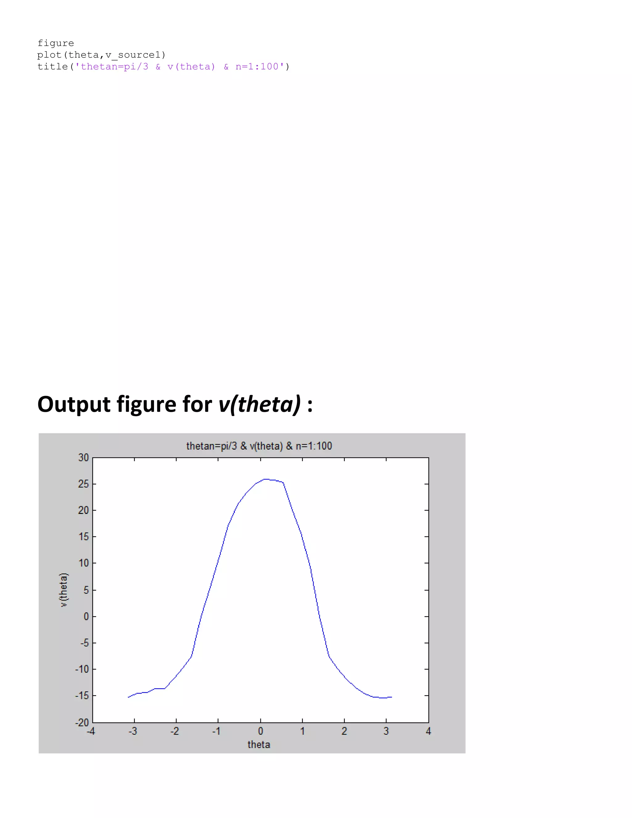
![Matlab code for v(theta) :
theta = linspace((-pi),(pi),length(theta1));
M=10;
N=100;
k=(2*M*thetan)/(2);
for l=1:length(theta)
for n=1:N
rR=0.6;
xn=0.1;
yn=0.1;
A=(rR+(xn*cos(theta(l)))+(yn*sin(theta(l))));
B=tan(n*theta(l));
C=((xn*sin(theta(l)))+(yn*cos(theta(l))));
D=sin(n*thetan/2)/(n*thetan/2);
k_n=(D*((2*A)/(A-B*C))*(rR^n));
segma(n)=k_n*cos(n*theta(l));
end
segma=sum(segma);
v_source1(l)=k*segma;
end
v_source1([ 9 22]) = 0;
v_source1([4 5 ]) = -13.7;](https://image.slidesharecdn.com/247606d7-733d-4cc8-b631-063f4bd57645-150513232406-lva1-app6891/75/ECG-graduation-project-69-2048.jpg)
![Neural networks background
The term neural network was traditionally used to refer to a network or circuit of biological neurons.
[1]
The modern usage of the term often refers
to artificial neural networks, which are composed of artificial neurons or nodes. Thus the term has two distinct usages
1. Biological neural networks are made up of real biological neurons that are connected or functionally related in a nervous system. In the field
of neuroscience, they are often identified as groups of neurons that perform a specific physiological function in laboratory analysis.
2. Artificial neural networks are composed of interconnecting artificial neurons (programming constructs that mimic the properties of biological
neurons). Artificial neural networks may either be used to gain an understanding of biological neural networks, or for solving artificial
intelligence problems without necessarily creating a model of a real biological system. The real, biological nervous system is highly complex:
artificial neural network algorithms attempt to abstract this complexity and focus on what may hypothetically matter most from an information
processing point of view. Good performance (e.g. as measured by good predictive ability, low generalization error), or performance mimicking
animal or human error patterns, can then be used as one source of evidence towards supporting the hypothesis that the abstraction really
captured something important from the point of view of information processing in the brain. Another incentive for these abstractions is to
reduce the amount of computation required to simulate artificial neural networks, so as to allow one to experiment with larger networks and
train them on larger data sets.
- An artificial neural network involves a network of simple processing elements (artificial neurons) which can exhibit complex global behavior,
determined by the connections between the processing elements and element parameters. Artificial neurons were first proposed in 1943
by Warren McCulloch, a neurophysiologist, and Walter Pitts, a logician, who first collaborated at the University of Chicago
Applications of natural and of artificial neural networks
The utility of artificial neural network models lies in the fact that they can be
used to infer a function from observations and also to use it. Unsupervised
neural networks can also be used to learn representations of the input that
capture the salient characteristics of the input distribution, e.g., see the
Boltzmann machine (1983), and more recently, deep learning algorithms, which
can implicitly learn the distribution function of the observed data. Learning in
neural networks is particularly useful in applications where the complexity of the
data or task makes the design of such functions by hand impractical.
The tasks to which artificial neural networks are applied tend to fall within the
following broad categories:
- Function approximation, or regression analysis, including time series prediction and modeling.
- Classification, including pattern and sequence recognition, novelty detection and sequential decision making.
- Data processing, including filtering, clustering, blind signal separation and compression.
Application areas of ANNs include system identification and control (vehicle control, process control), game-playing and
decision making (backgammon, chess, racing), pattern recognition (radar systems, face identification, object
recognition), sequence recognition (gesture, speech, handwritten text recognition), medical diagnosis, financial
applications, data mining (or knowledge discovery in databases, "KDD"), visualization and e-mail spam filtering.
Models
Neural network models in artificial intelligence are usually referred to as artificial neural networks (ANNs); these are essentially simple mathematical
models defining a function or a distribution over or both and , but sometimes models are also intimately associated with a particular
learning algorithm or learning rule. A common use of the phrase ANN model really means the definition of a class of such functions (where members of
the class are obtained by varying parameters, connection weights, or specifics of the architecture such as the number of neurons or their connectivity).
- Network function
The word network in the term 'artificial neural network' refers to the inter–connections between the neurons in the different layers of each
system. An example system has three layers. The first layer has input neurons, which send data via synapses to the second layer of neurons,
and then via more synapses to the third layer of output neurons. More complex systems will have more layers of neurons with some having](https://image.slidesharecdn.com/247606d7-733d-4cc8-b631-063f4bd57645-150513232406-lva1-app6891/75/ECG-graduation-project-71-2048.jpg)
![increased layers of input neurons and output neurons. The synapses store
parameters called "weights" that manipulate the data in the calculations.
An ANN is typically defined by three types of parameters:
1. The interconnection pattern between different layers of neurons
2. The learning process for updating the weights of the interconnections
3. The activation function that converts a neuron's weighted input to its
output activation.
Mathematically, a neuron's network function is defined as a
composition of other functions , which can further be defined as a
composition of other functions. This can be conveniently represented as a
network structure, with arrows depicting the dependencies between
variables. A widely used type of composition is the nonlinear weighted
sum, where , where (commonly referred
to as the activation function
[1]
) is some predefined function, such as
the hyperbolic tangent. It will be convenient for the following to refer to a
collection of functions as simply a vector .
This figure depicts such a decomposition of , with dependencies
between variables indicated by arrows. These can be interpreted in two
ways.
. The first view is the functional view: the input is transformed into a 3-
dimensional vector , which is then transformed into a 2-dimensional
vector , which is finally transformed into . This view is most commonly encountered in the context of optimization.
. The second view is the probabilistic view: the random variable depends upon the random variable , which depends
upon , which depends upon the random variable . This view is most commonly encountered in the context of graphical models.
The two views are largely equivalent. In either case, for this particular network architecture, the components of individual layers are
independent of each other (e.g., the components of are independent of each other given their input ). This naturally enables a degree of
parallelism in the implementation.
Networks such as the previous one are commonly called feedforward, because their graph is a directed acyclic graph. Networks
with cycles are commonly called recurrent. Such networks are commonly depicted in the manner shown at the top of the figure, where is
shown as being dependent upon itself. However, an implied temporal dependence is not shown.
- Learning
What has attracted the most interest in neural networks is the possibility of learning. Given a specific task to solve, and a class of functions
, learning means using a set of observations to find which solves the task in some optimal sense.
This entails defining a cost function such that, for the optimal solution , - i.e., no solution has a cost
less than the cost of the optimal solution
The cost function is an important concept in learning, as it is a measure of how far away a particular solution is from an optimal solution to the
problem to be solved. Learning algorithms search through the solution space to find a function that has the smallest possible cost.
For applications where the solution is dependent on some data, the cost must necessarily be a function of the observations, otherwise we would not be
modelling anything related to the data. It is frequently defined as a statistic to which only approximations can be made. As a simple example, consider
the problem of finding the model , which minimizes , for data pairs drawn from some distribution . In practical
situations we would only have samples from and thus, for the above example, we would only minimize . Thus,
the cost is minimized over a sample of the data rather than the entire data set.](https://image.slidesharecdn.com/247606d7-733d-4cc8-b631-063f4bd57645-150513232406-lva1-app6891/75/ECG-graduation-project-72-2048.jpg)
![When some form of online machine learning must be used, where the cost is partially minimized as each new example is seen. While online
machine learning is often used when is fixed, it is most useful in the case where the distribution changes slowly over time. In neural network
methods, some form of online machine learning is frequently used for finite datasets.
- Learning paradigms
Supervised learning
Unsupervised learning
Reinforcement learning
- Learning algorithms
Training a neural network model essentially means selecting one model from the set of allowed models (or, in a Bayesian framework,
determining a distribution over the set of allowed models) that minimizes the cost criterion. There are numerous algorithms available for
training neural network models; most of them can be viewed as a straightforward application of optimization theory and statistical estimation.
Most of the algorithms used in training artificial neural networks employ some form of gradient descent. This is done by simply taking the
derivative of the cost function with respect to the network parameters and then changing those parameters in a gradient-related direction.
Evolutionary methods, simulated annealing, expectation-maximization, non-parametric methods and particle swarm optimization are some
commonly used methods for training neural networks.
Employing artificial neural networks
Perhaps the greatest advantage of ANNs is their ability to be used as an arbitrary function approximation mechanism that 'learns' from observed data.
However, using them is not so straightforward and a relatively good understanding of the underlying theory is essential.
Choice of model: This will depend on the data representation and the application. Overly complex models tend to lead to problems with learning.
Learning algorithm: There are numerous trade-offs between learning algorithms. Almost any algorithm will work well with
the correct hyperparameters for training on a particular fixed data set. However selecting and tuning an algorithm for training on unseen data
requires a significant amount of experimentation.
Robustness: If the model, cost function and learning algorithm are selected appropriately the resulting ANN can be extremely robust.
With the correct implementation, ANNs can be used naturally in online learning and large data set applications. Their simple implementation and the
existence of mostly local dependencies exhibited in the structure allows for fast, parallel implementations in hardware.
In the task at hand we used a NN simulator Inserting a data set based on the equation :
v=[(sin(n*thetan/2))/(n*thetan/2)]*(rR^n)*cos(n*theta)](https://image.slidesharecdn.com/247606d7-733d-4cc8-b631-063f4bd57645-150513232406-lva1-app6891/75/ECG-graduation-project-73-2048.jpg)


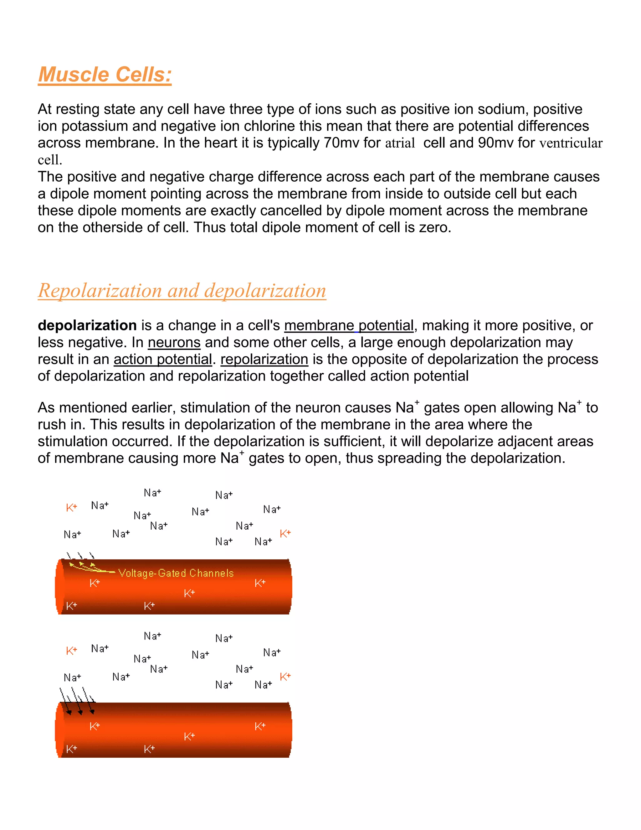
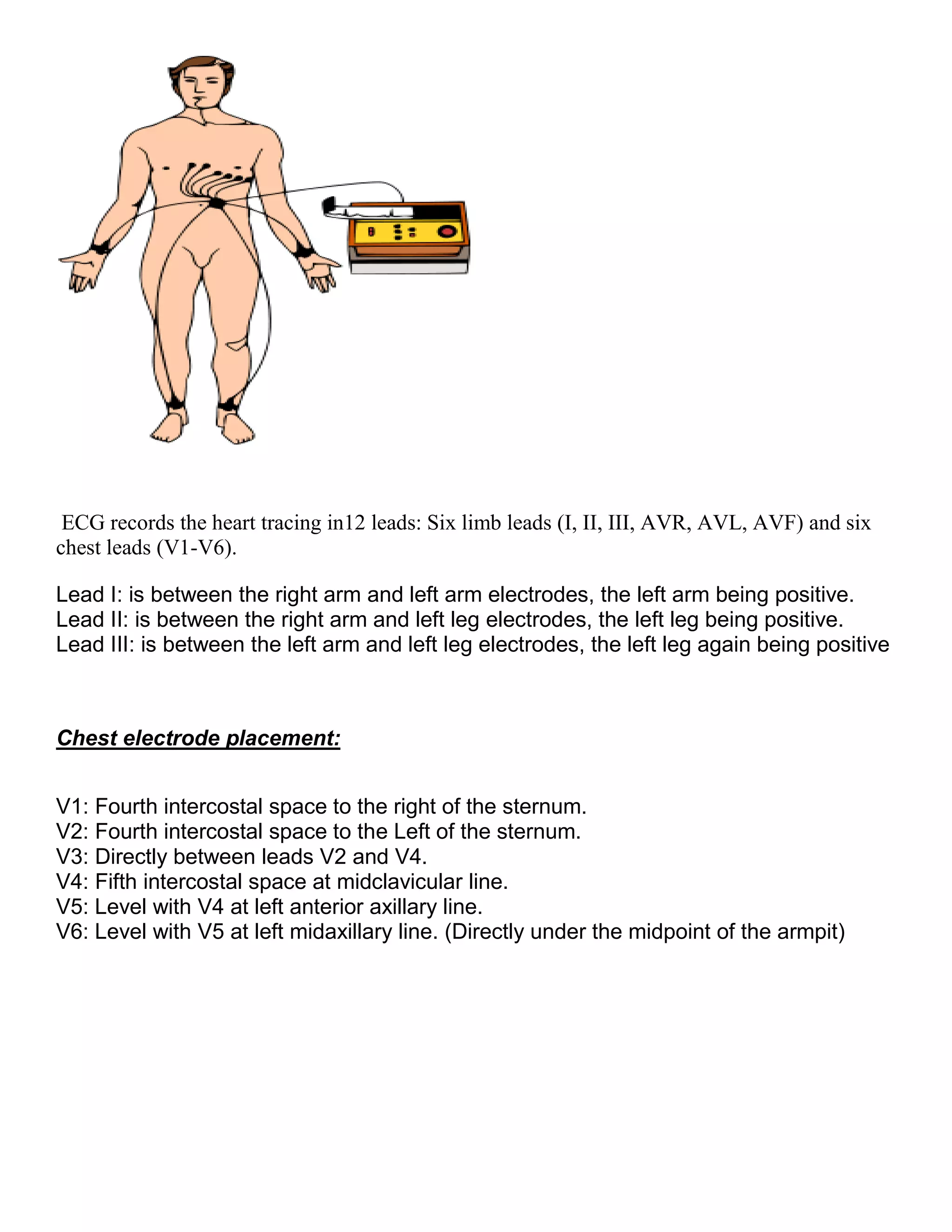
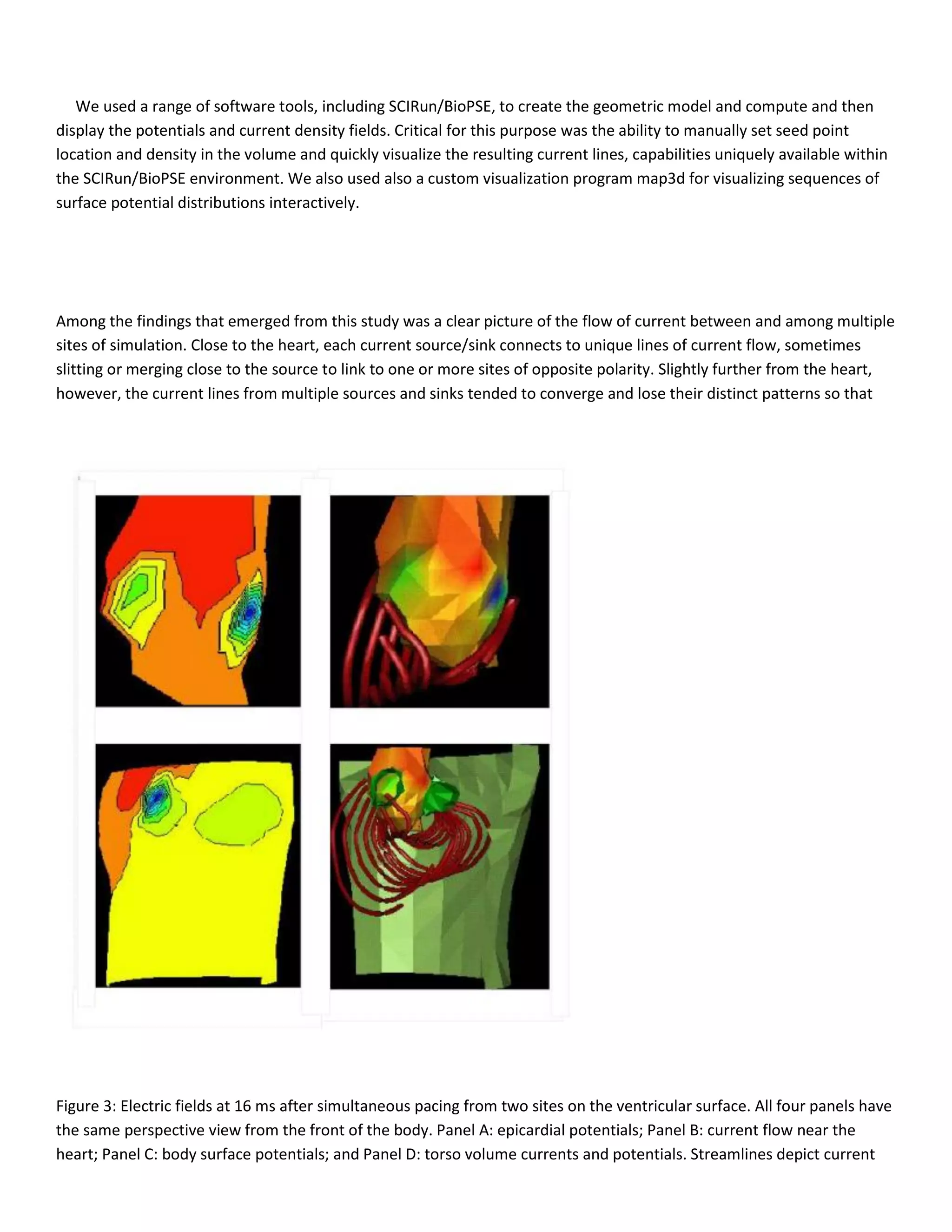
This document provides an introduction to electrocardiography (ECG) and the electrical properties of the human heart. It discusses the structure and function of the heart chambers and valves. It describes how electrical impulses are generated in the sinoatrial node and propagated through the heart muscle to coordinate contractions. Recording these electrical signals noninvasively with electrodes on the skin is the basis of ECG. Key events in the cardiac cycle such as depolarization and repolarization are also summarized.


