


![ Durbin h test (1-d/2)[n/1-n{var(αt-1 )} ]1/2
Durbin h test (0.4972) [(30/1-30(0.239) ]1/2
Durbin h test 5.1191
( Durbin h ~ Norm distribution , As h value exceed ±3 , so the probability is highly significant
Decision:
There is a positive autocorrelation ,
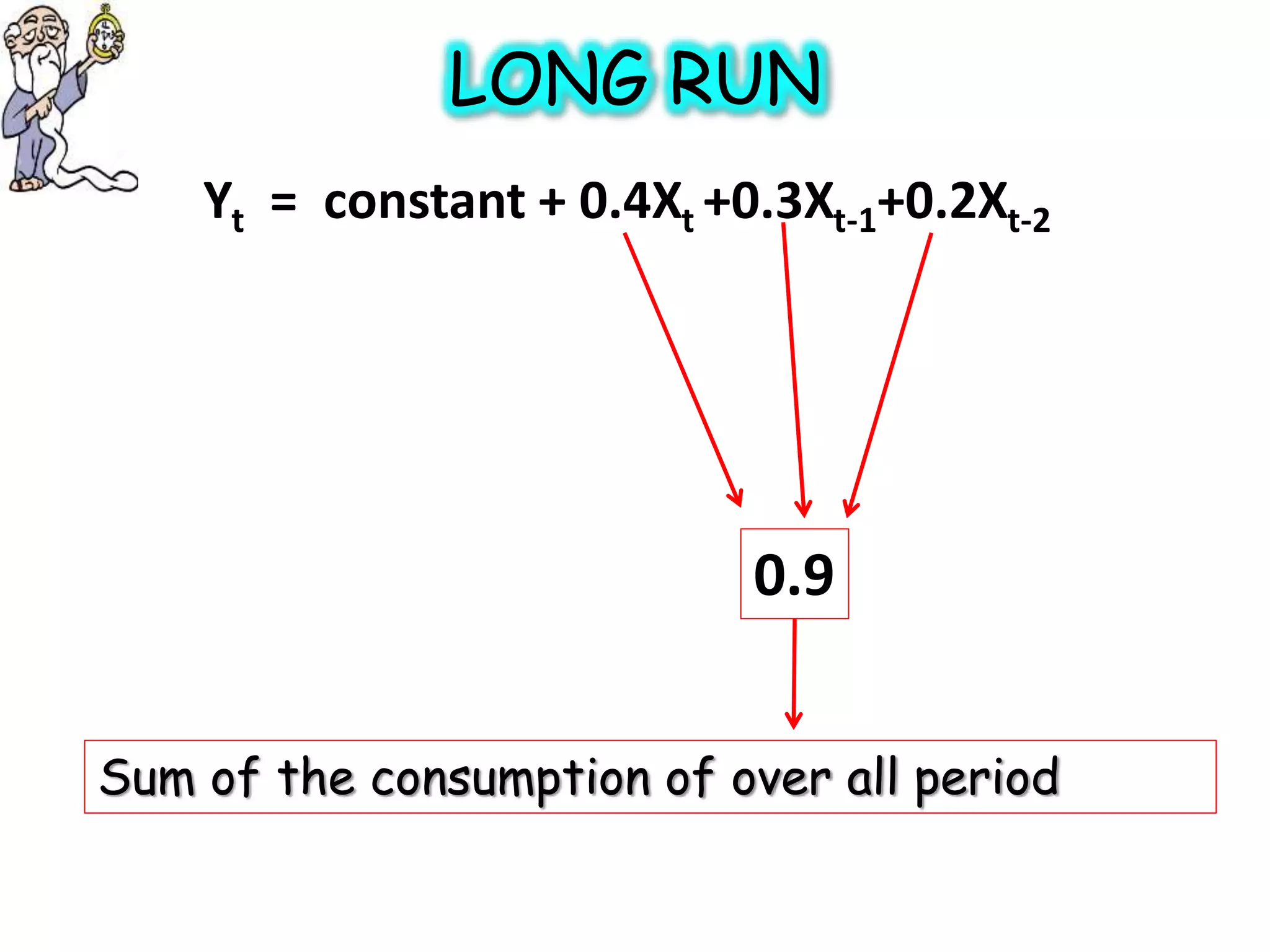
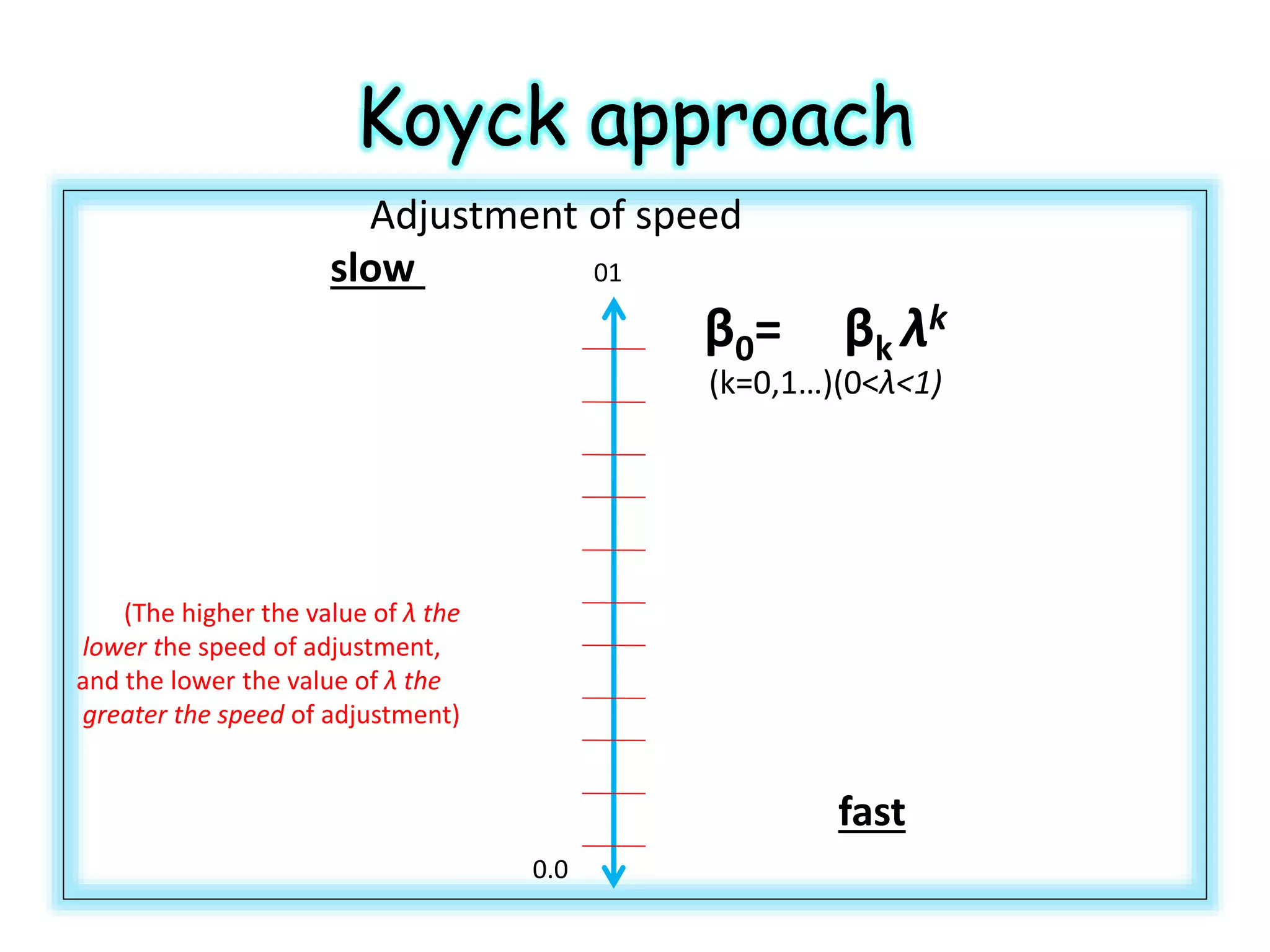
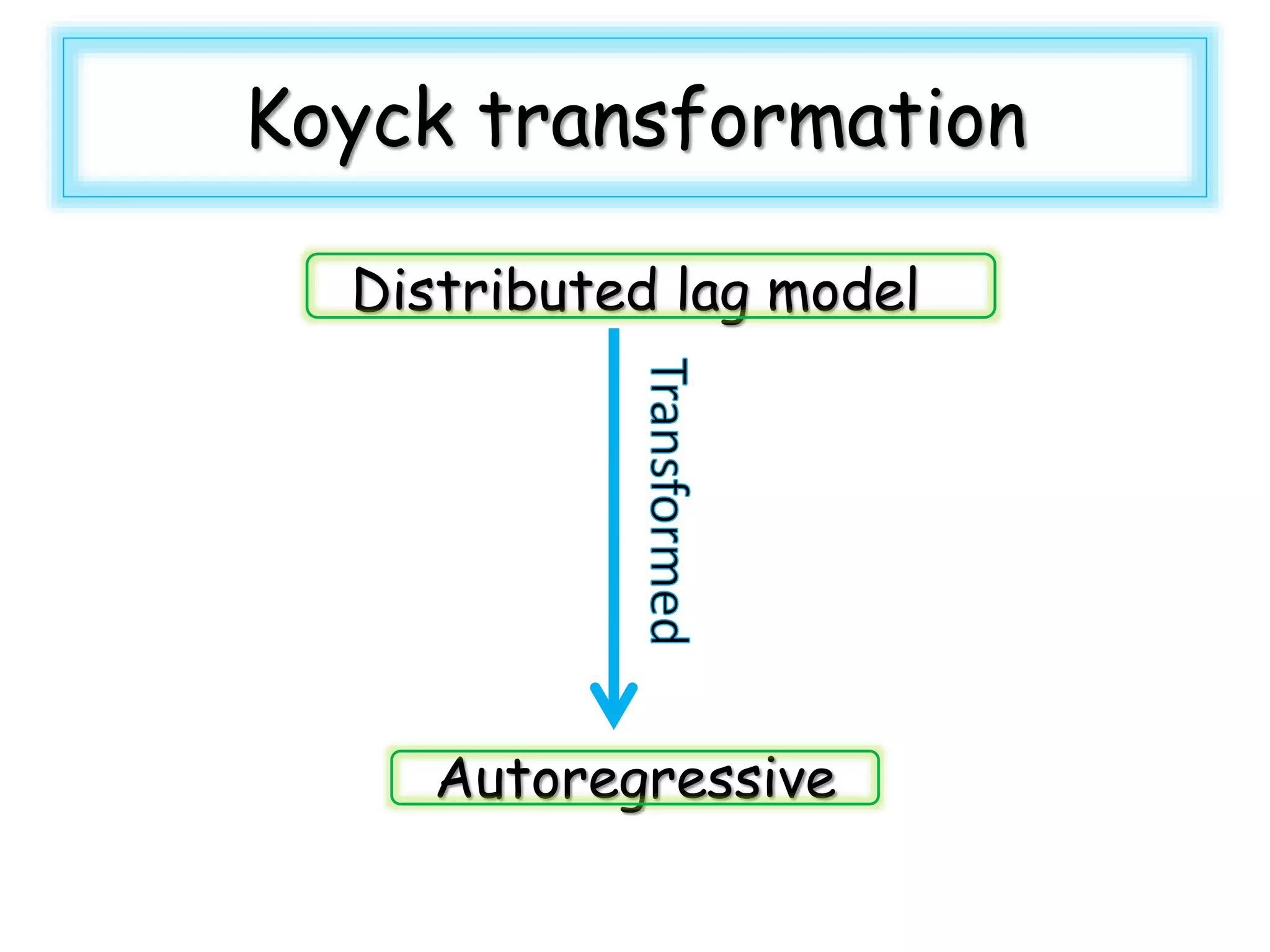
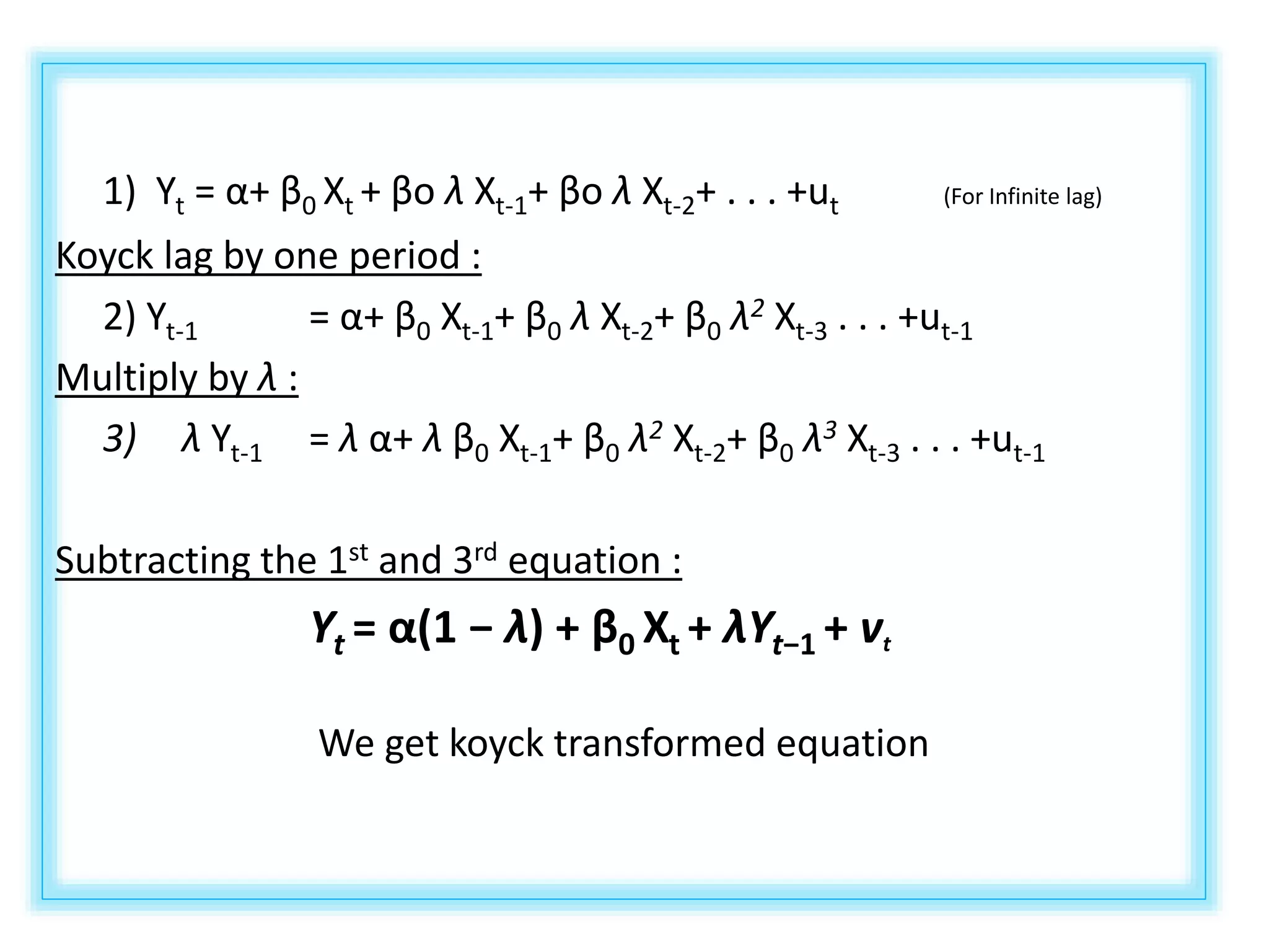
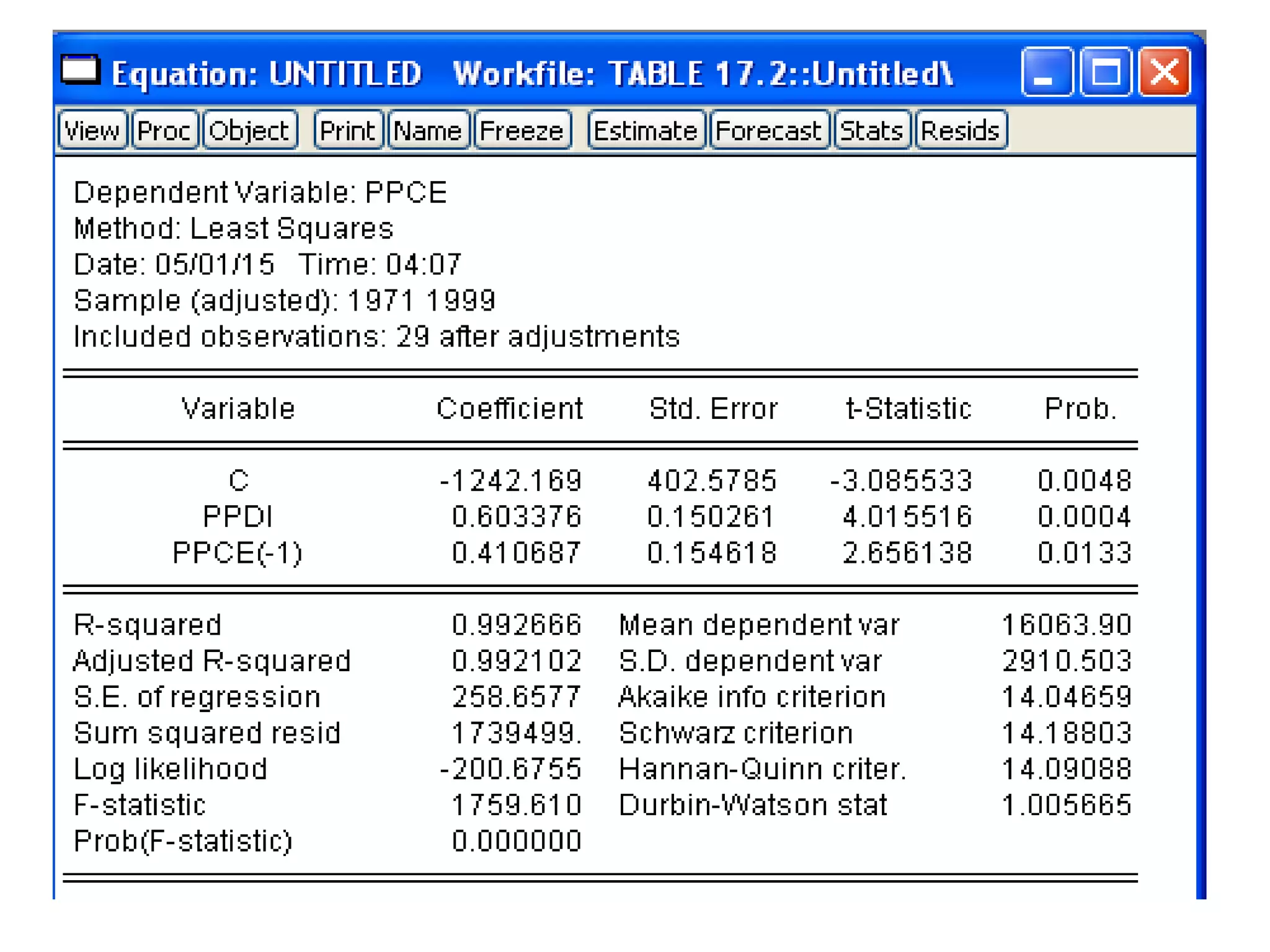
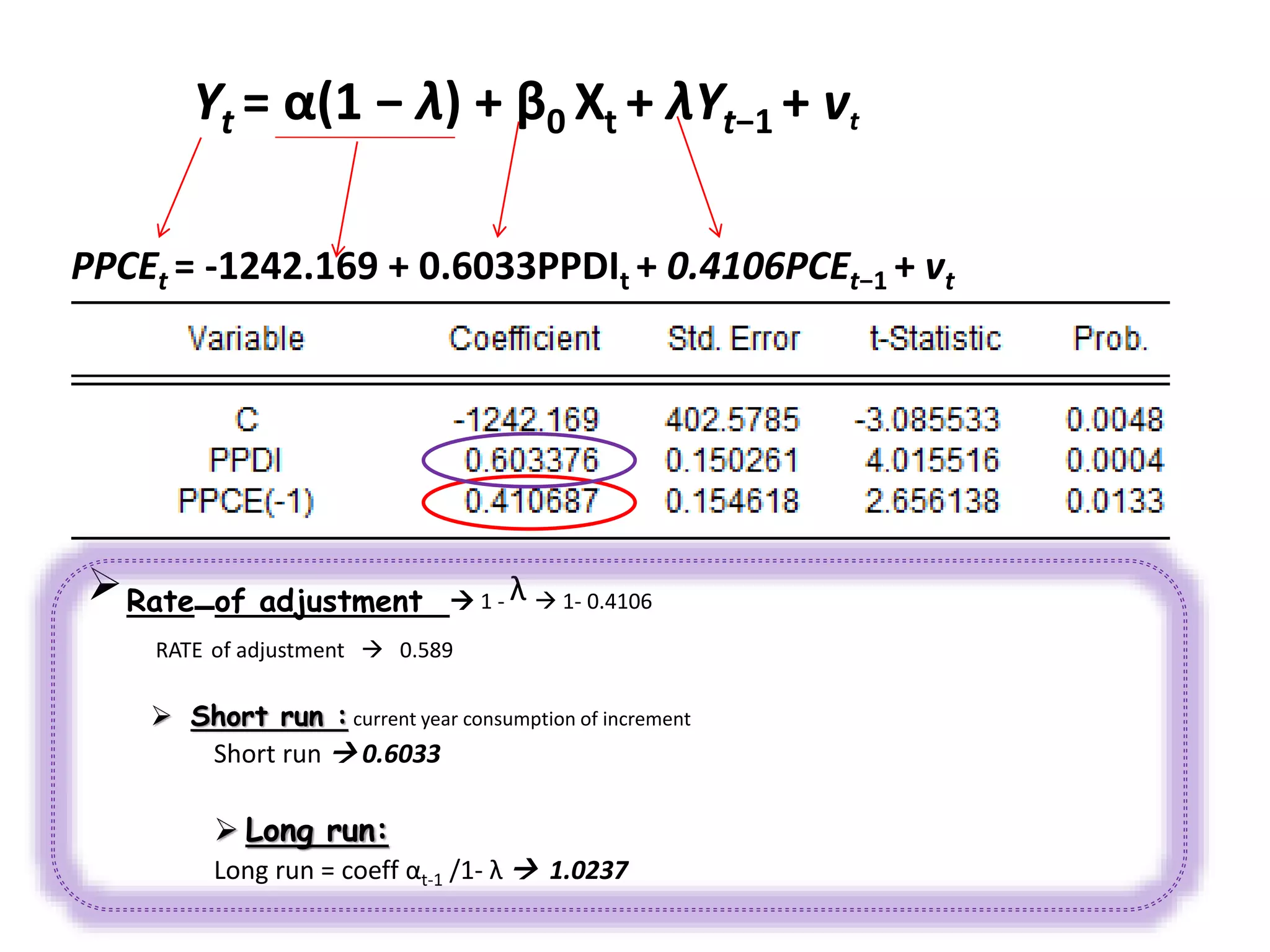
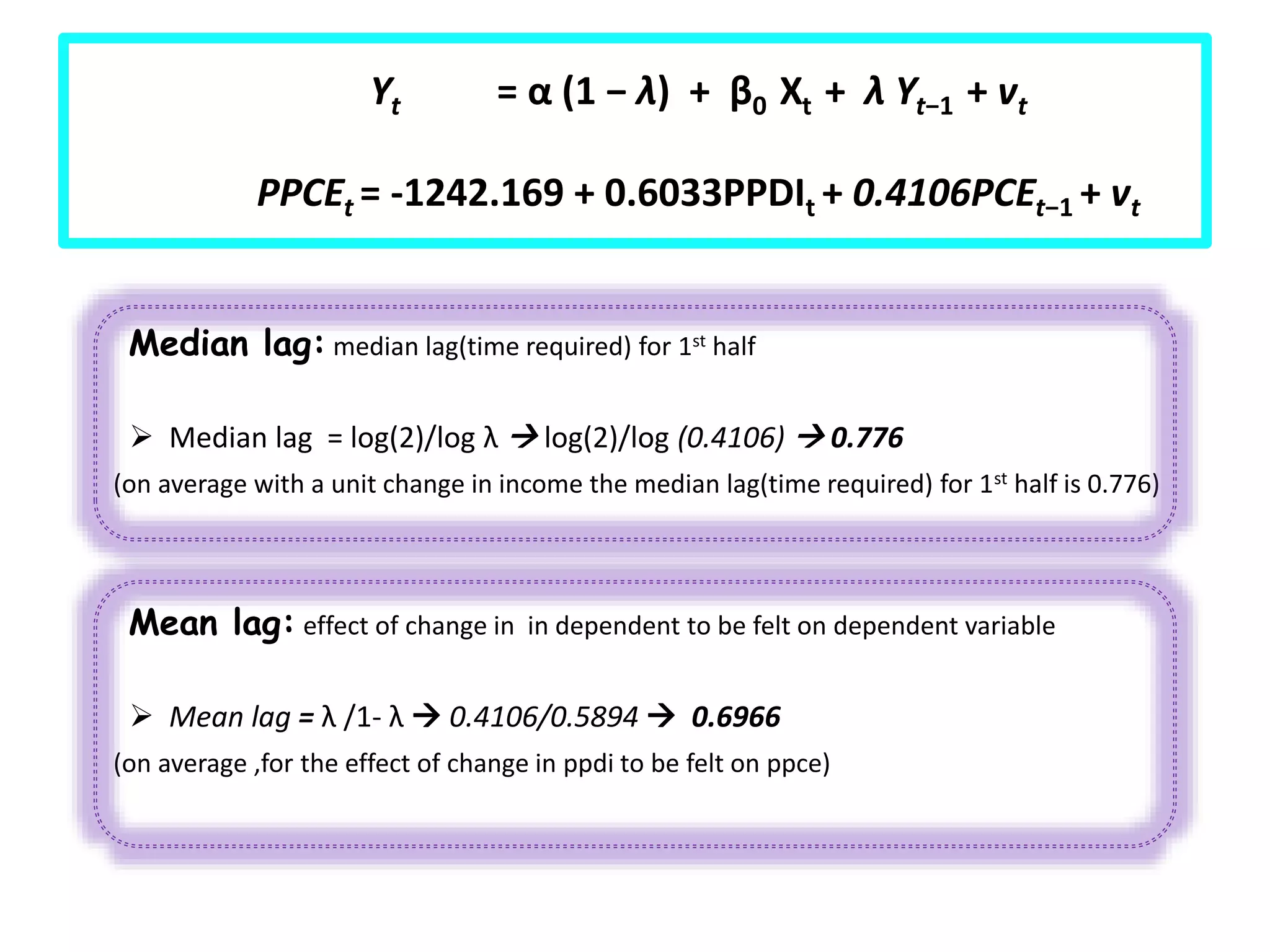
Yt = α (1 − λ) + β0 Xt + λ Yt−1 + vt
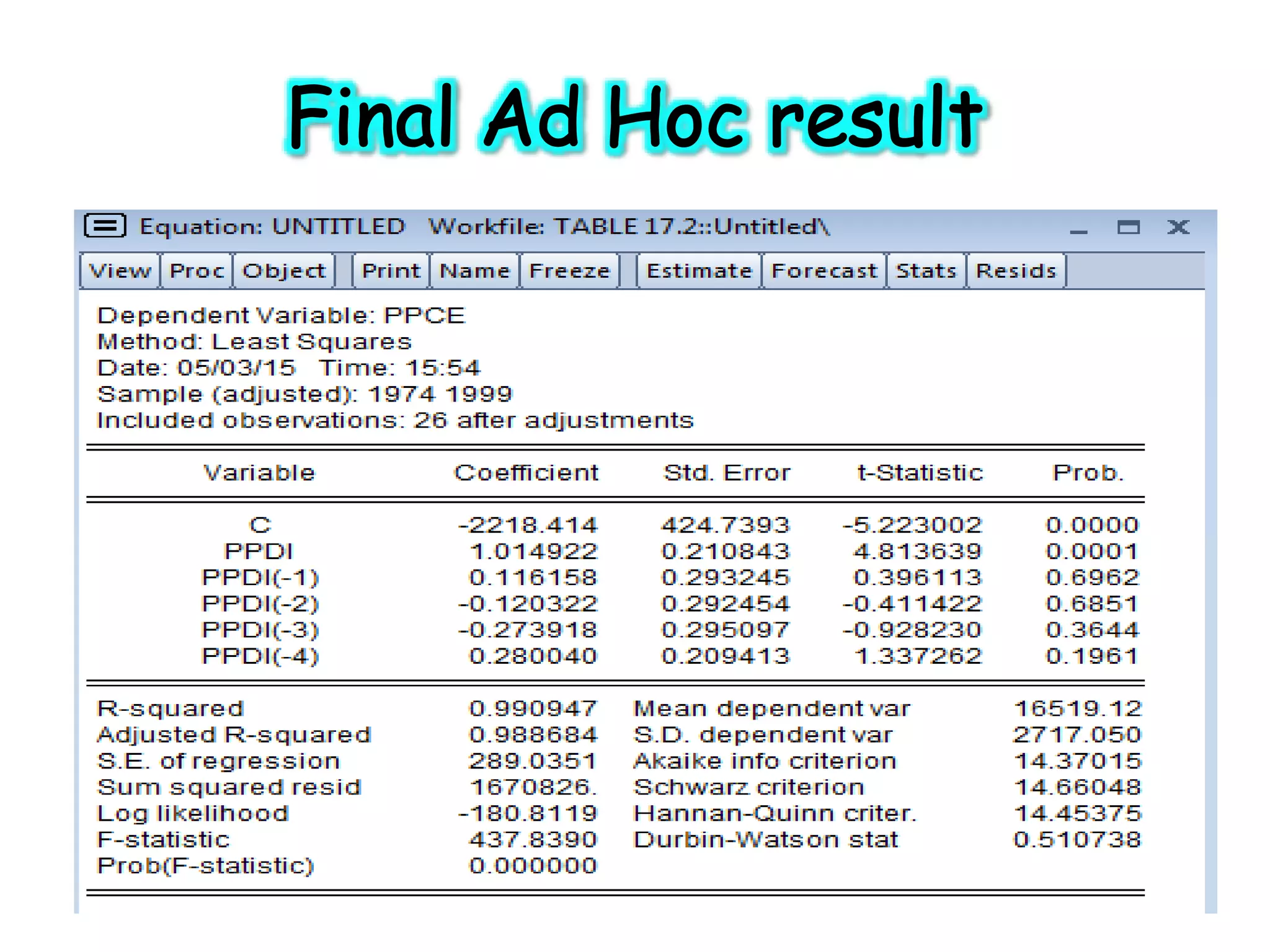
PPCEt = -1242.169 + 0.6033PPDIt + 0.4106PCEt−1 + vt](https://image.slidesharecdn.com/finaldynamicppt-151220101447/75/DYNAMIC-ECONOMETRIC-MODELS-BY-Ammara-Aftab-49-2048.jpg)


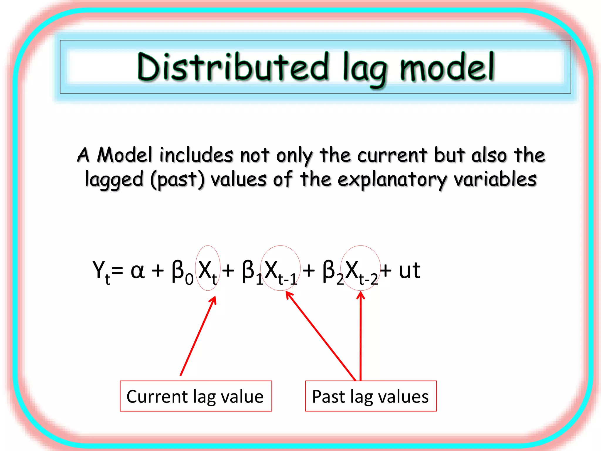
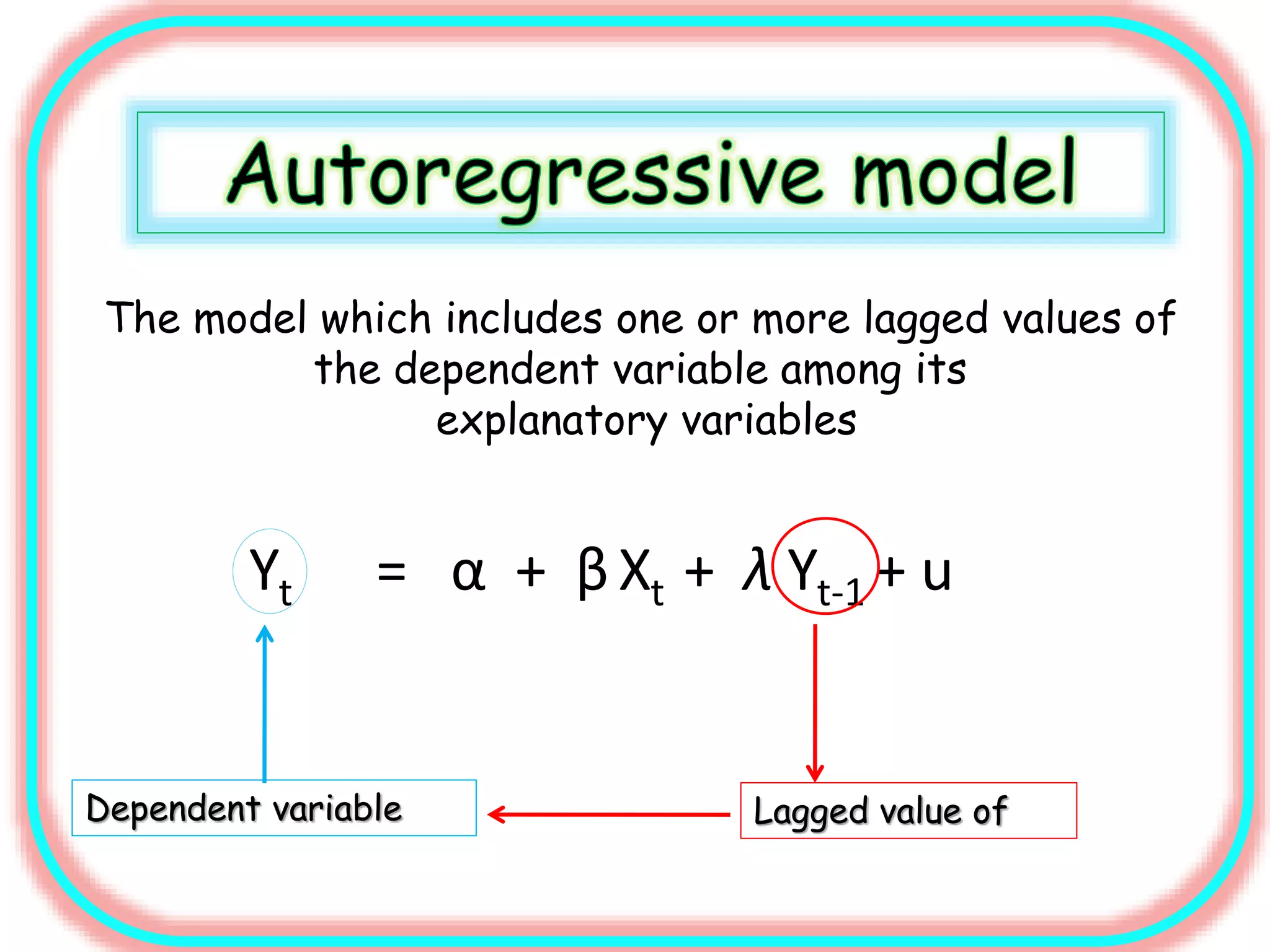
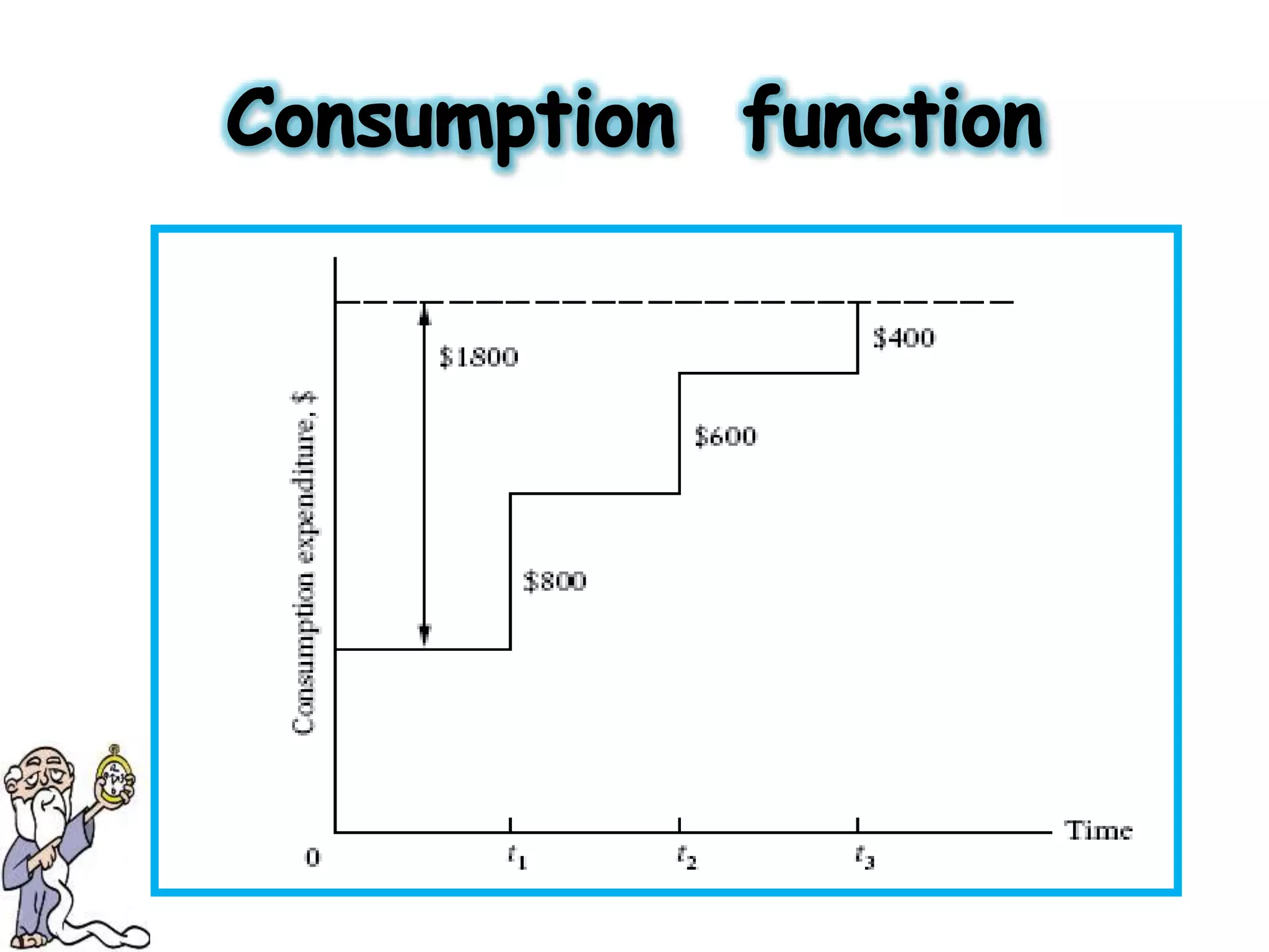
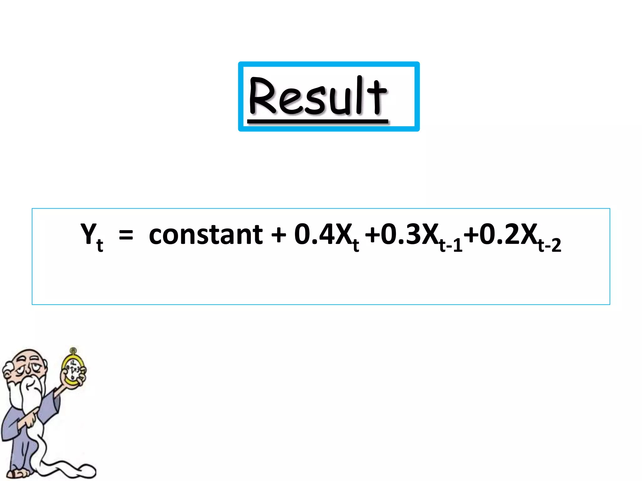
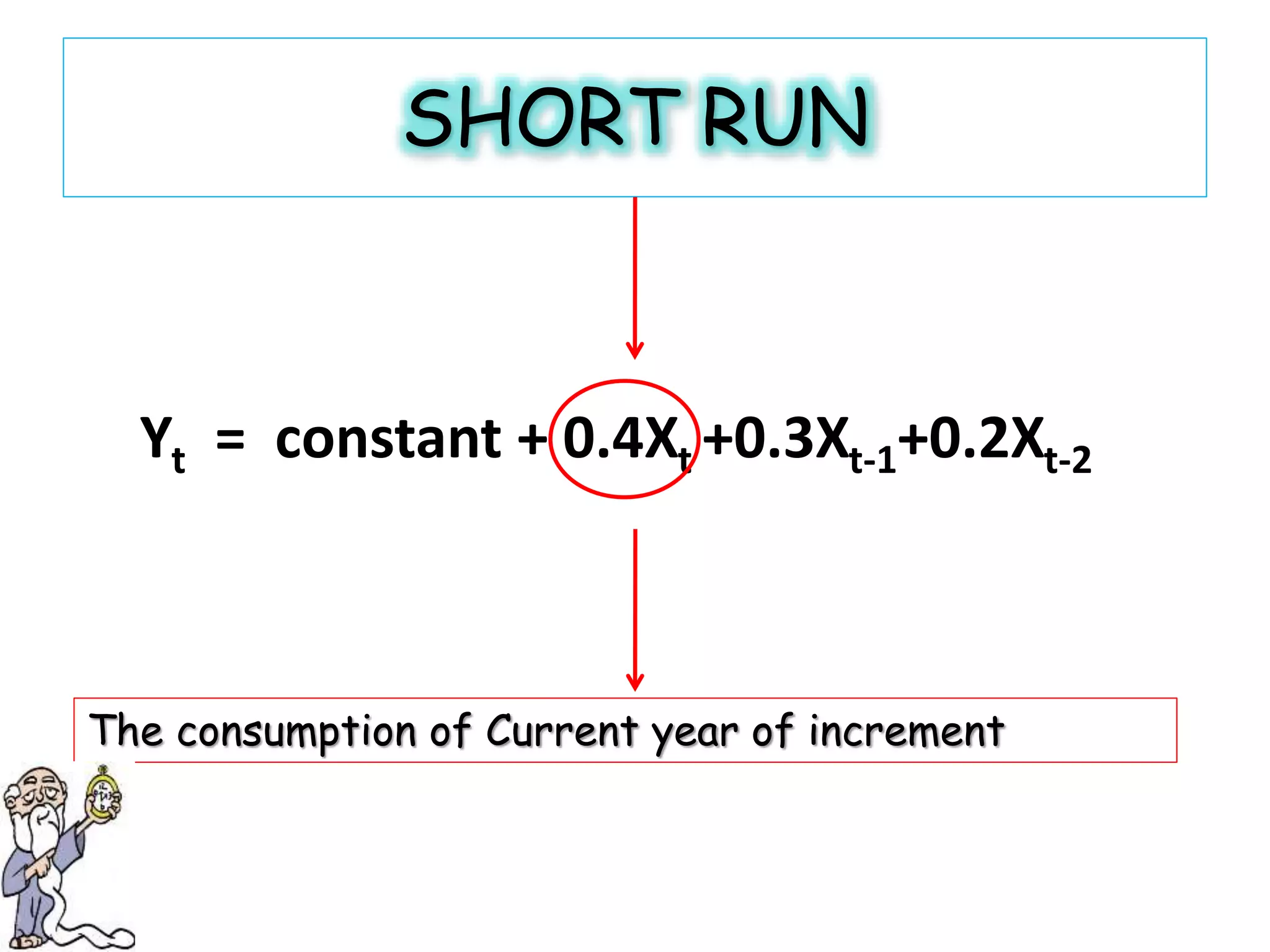
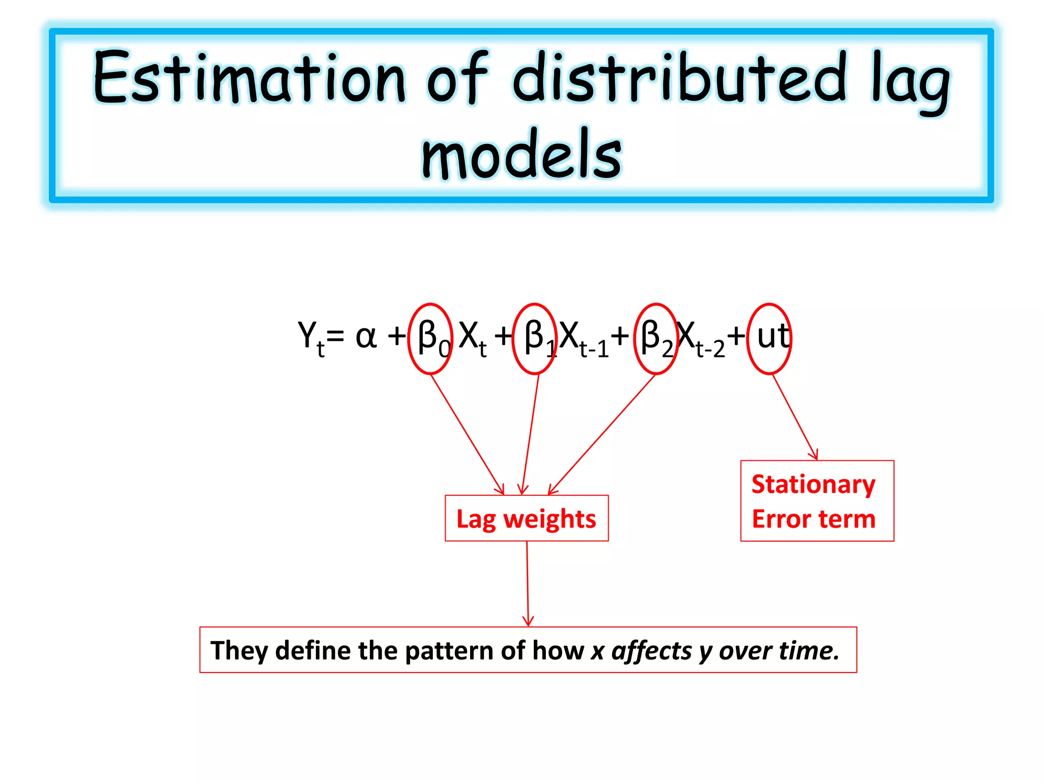
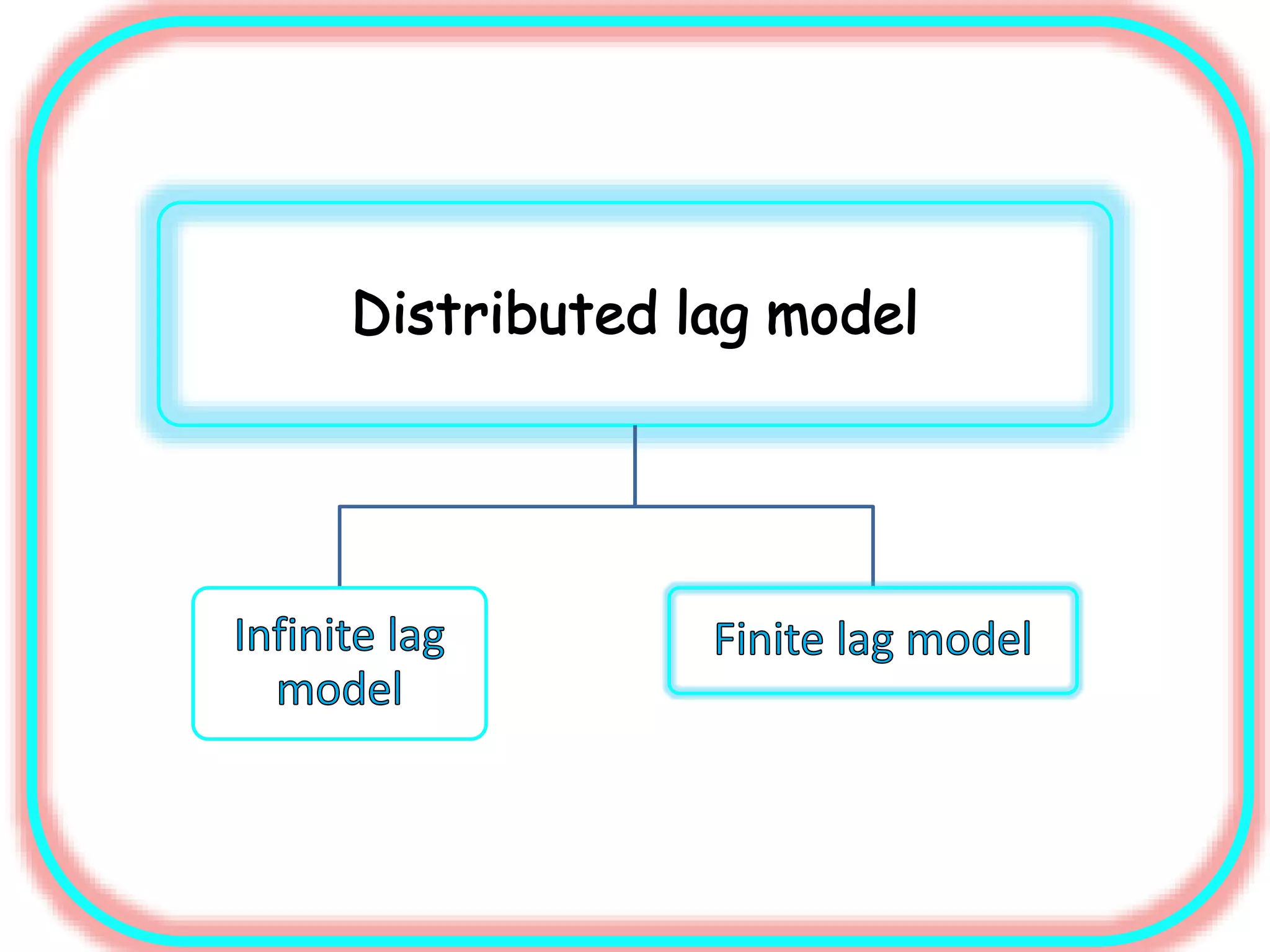
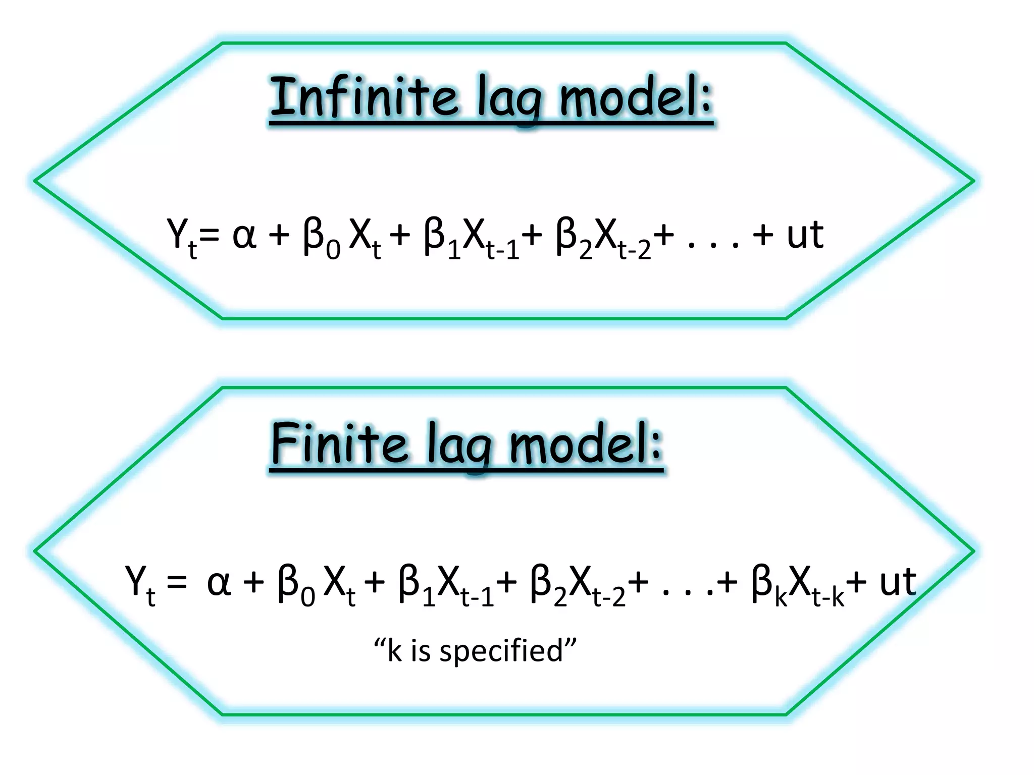
The document discusses the role of lags in economic models. Lags refer to past values of variables that are used to predict current or future values. Models with lags are used to capture delayed effects, where a change in one variable impacts another variable after some time. Specifically, the document discusses: 1) Distributed lag models which include current and past lagged values of explanatory variables to predict a dependent variable. 2) Models with lagged dependent variables to capture partial adjustment effects, where changes in a variable adjust gradually over time rather than immediately. 3) The Koyck transformation allows estimating the long run impact of a variable from the lag structure in these partial adjustment models. Lags are widely used