Downloaded 11 times
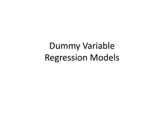

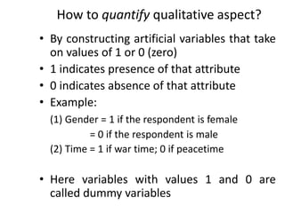
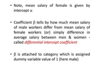
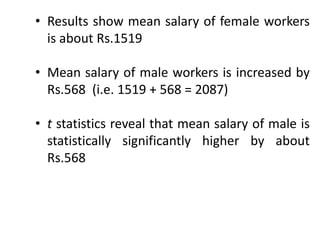
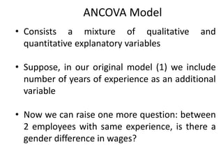
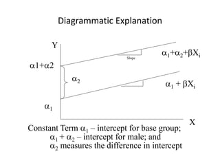
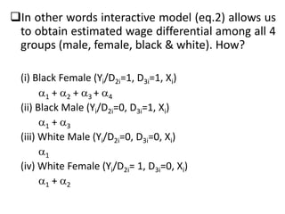
![• Hence, we describe gender using dummy
variable
D = 1 if male respondent
= 0 if female respondent [reference group]
Let the regression model as
Yi = + D + ui (1)
(where Y-Monthly salary)](https://image.slidesharecdn.com/dummyvariable1-210921030628/85/Dummyvariable1-8-320.jpg)
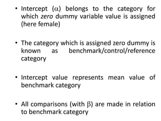
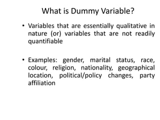
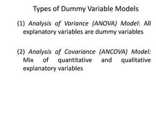
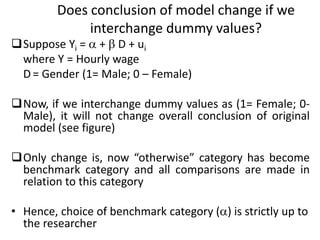
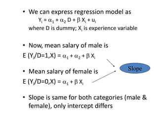
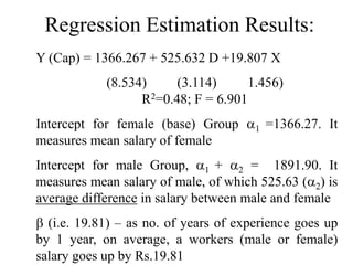
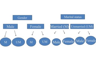
![• Hypothesis testing:
• Done in the usual way
• H0 : = 0 [No gender discrimination in salary
determination/no statistically significant
difference in salaries between males and
females]
• H1 : 0 [Gender discrimination is present in
salary determination]
• Use t – statistics
• If is significantly different from zero, we can
accept alternate hypothesis](https://image.slidesharecdn.com/dummyvariable1-210921030628/85/Dummyvariable1-12-320.jpg)
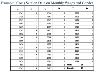
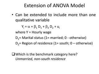

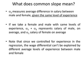
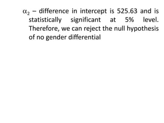
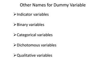
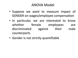
![Interactions Involving Dummy Variables
• Consider the following model:
Yi = 1 + 2 D2i + 3 D3i + Xi + ui ----- (1)
Yi = Hourly wage
Xi = Education (years of schooling)
D2 = 1 if female, 0 if male [GENDER]
D3 = 1 if black, 0 if white [RACE]
Note that in this model dummy variables are
interactive in nature. How?](https://image.slidesharecdn.com/dummyvariable1-210921030628/85/Dummyvariable1-30-320.jpg)
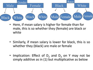

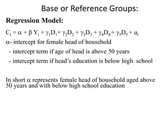
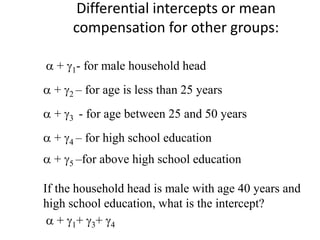
Dummy variables allow qualitative or categorical variables to be included in regression models. They take values of 0 and 1 to indicate absence or presence of a characteristic. The document discusses different types of dummy variable models including ANOVA models with all dummy explanatory variables and ANCOVA models with both dummy and quantitative variables. It provides an example of an ANOVA model to examine gender discrimination in wages. Coefficients on dummy variables represent differences in intercepts between categories. Interactive dummy variable models allow examination of effects that vary across categories of two or more qualitative variables, such as differences in wages between gender-race groups. Choice of reference categories does not change overall conclusions.


![제 23회 보아즈(BOAZ) 빅데이터 컨퍼런스 - [MBOAX] : ABSA를 활용한 소비자 반응 분석 기반 운영 효율화 대시보드 설계](https://cdn.slidesharecdn.com/ss_thumbnails/3-1boaz23rdconferencemboax-260203102709-9d519923-thumbnail.jpg?width=640&height=640&fit=bounds)


