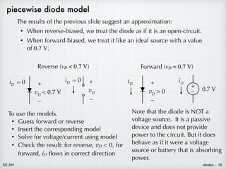
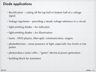
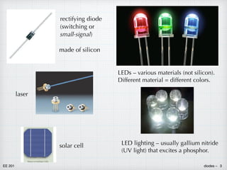
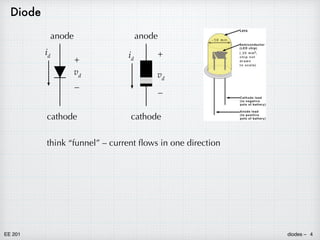
Diodes are two-terminal semiconductor devices that allow current to flow easily in one direction but restrict it in the other. They are made of materials like silicon and germanium. A diode consists of a p-n junction where a p-type semiconductor is joined to an n-type semiconductor. Diodes have highly non-linear current-voltage characteristics that make circuit analysis difficult. However, diodes can be approximated as an open circuit when reverse biased and a 0.7V voltage source when forward biased, simplifying analysis. This piecewise linear model provides results close to the exact solution with much less effort.

1. EE 201 diodes – 1
Diodes
Diodes are two-terminal electronic devices, made out of a
semiconductor materials. Silicon is the most common semiconductor,
but there are others, like germanium, gallium arsenide (GaAs), indium
phosphide (InP), gallium nitride (GaN), and many others.
Semiconductors are interesting because their electrical properties can
be varied over many order of magnitude: resistivity as high as 107 Ω-m
(almost an insulator) or as low as 10–6 Ω-m (almost a conductor).
Also, semiconductors can be made in two different “varieties”: either n-
type in which current is carried by electrons – as usual – or p-type, in
which current behaves like it is carried by positive charges, which we
cal “holes”.
A diode consists of a layer of n-type joined to a layer of p-type material
creating a p-n junction. When a voltage is applied across the junction, a
current flows in response, but the i-v relationship is extremely non-
linear. The non-linearity will force us to modify our approach to
analyzing circuits.

2. EE 201 diodes – 2
Diode applications
• Rectification – cutting off the top half or bottom half of a voltage
signal.
• Voltage regulation – providing a steady voltage reference in a circuit.
• light-emitting diodes – for indicators
• light-emitting diodes – for illumination
• lasers - DVD players, fiber-optic communication, surgery
• photodetectors – sense presence of light, especially low levels or fast
pulses
• photovoltaics (solar cells) – “green” electrical power generation
• building block for transistors

3. EE 201 diodes – 3
rectifying diode
(switching or
small-signal)
made of silicon
LEDs – various materials (not silicon).
Different material = different colors.
LED lighting – usually gallium nitride
(UV light) that excites a phosphor.
laser
solar cell

4. EE 201 diodes – 4
id
+
–
vd
Diode
anode
cathode
anode
cathode
–
vd
+
id
think “funnel” – current flows in one direction

5. EE 201 diodes – 5
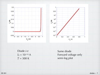
diode i-v characteristic id
+
–
vd
The ideal diode equation:
where iD is the diode current and vD voltage across the diode. As stated
earlier, the relationship is extremely non-linear, and it will cause us a some
grief when analyzing diodes. But the non-linear behavior offers
opportunities for new applications.
• IS is the current parameter of the diode, often known as the saturation
current or scale current. It is like “R” for a resistor. Each diode will
have a unique value for IS. A typical value is IS ≈ 10–14 A.
• kT/q is the thermal voltage. k is Boltzmann’s constant (recall
thermodynamics from physics) with a value of 1.38x10–23 J/K. T is the
absolute temperature of the diode, expressed in kelvin (K). Then the
product kT is the thermal energy and represents the average energy of
an electron in the semiconductor. If we divide the electron the
electron charge — q = 1.6x10–19 C — we get the thermal voltage. At
300 K (= 27°C, approximately room temperature), kT/q = 25.8 mV.
iD = IS
[
exp
(
vD
kT/q)
− 1
]

6. EE 201 diodes – 6
diode: forward and reverse conduction
id
+
–
vd
If vD is more positive than about 3·kT/q (≈ 75 mV at room temperature.)
Current increases exponentially with
increasing voltage. This is forward bias
or forward conduction.
If vD is more negative than about –3·kT/q
A very small trickle of current flows — almost
zero. The current is independent of voltage.
This is reverse bias.
In an ideal diode, current essentially flows in only one direction. This is
asymmetry is the basis for some of the important applications of diodes.
(We will see later that current can flow in the reverse direction in the
right circumstances.
iD = IS
[
exp
(
vD
kT/q)
− 1
]
iD ≈ IS exp
(
vD
kT/q )
iD ≈ − IS

7. EE 201 diodes – 7
-0.05
0
0.05
0.1
0.15
0.2
0.25
0.3
-3 -2.5 -2 -1.5 -1 -0.5 0 0.5 1
I
D
(A)
V
D
(V)
10-14
10-12
10-10
10-8
10-6
10-4
0.01
1
0 0.2 0.4 0.6 0.8 1
I
D
(A)
V
D
(V)
Diode i-v
IS = 10–14 A
T = 300 K
Same diode
Forward voltage only
semi-log plot

8. EE 201 diodes – 8
diodes in circuits
The non-linear behavior has some significant effects:
• Basic notions are still valid: KCL and KCL, energy, power.
• Node-voltage and mesh-current techniques are still applicable, but
they usually result in a set of non-linear equations, which are
difficult to solve.
• Techniques that rely on linearity — superposition and Thevenin
equivalents — cannot be applied directly when non-linear elements
are present.
When analyzing circuits with non-linear elements, we will make use of:
• Approximations that simplify the non-linear behavior. Essentially
we will linearize the elements — hiding the exponential behavior
and allowing us to use our familiar techniques. This approximation
technique requires some initial guesses and the results must be
checked to confirm. Of course, it is only approximate.
• SPICE. It was invented to handle circuits with non-linear elements.

9. EE 201 diodes – 9
diodes in circuits
Important: When working with diodes, don’t EVER apply a forward
voltage directly across the diode. The result is usually a dead diode.
IS = 10–14 A
room temp: kT/q = 25.8 mV.
vD = VS
Of course, this is absolutely absurd. What really happens is that the
diode would rapidly heat up and burn out during the transient as the
current increased. There must always be something — probably a
resistor — to limit the current.
iD ≈ IS exp
(
vD
kT/q )
= (10−14
A) exp
[
1.5 V
0.0258 V]
= 1.8 × 1011
A = 180 GA
+
–
VS
1.5 V
iD
–
+
vD

10. EE 201 diodes – 10
So add a current-limiting resistor in series.
IS = 10–14 A.
kT/q = 25.8 mV.
VS – vR + vD = 0
VS − iDR − vD = 0
iD = IS
[
exp
(
vD
kT/q)
− 1
]
vD =
kT
q
ln
[
iD
IS
+ 1
]
VS − iDR −
kT
q
ln
[
iD
IS
+ 1
]
= 0
The result is a transcendental equation. It is a perfectly valid relationship
for which there is a unique value for the current, but we can’t solve it by
usual algebraic techniques. It is impossible. To find the the current, we
are forced to use numerical techniques, meaning that are we will use a
sequence of smart “trial-and-error” steps to determine the value of iD.
Numerical analysis is an important topic in computer programming. In
fact, computers were invented to solve math and physics problems that
were too difficult to do by hand. SPICE is essentially a specialized
numerical analysis app.
Yikes!
+
–
VS
1.5 V
iD
–
+
vD
R
1 kΩ

11. EE 201 diodes – 11
Crudely, we could make a guess for the value of iD and plug it into the
equation. Most likely, our guess will be wrong and the left side of the
equation will not equal zero. Based on the result, we can make a new
guess and try again. We keep repeating until we zero in — converge — on
the correct result. A well-written computer algorithm will take an initial
guess and then automatically converge on the correct result after some
number of iterations. The process stops when the change in the calculated
result from one step to the next is smaller than the desired precision.
There are many algorithms for finding zeros of an equation. One method
that we can apply here is fixed-point iteration. We start by re-writing the
transcendental equation,
iD =
VS
R
−
kT/q
R
ln
[
iD
IS
+ 1
]
= 1.5 mA − (0.0258 mA) ln
[
iD
10−11 mA
+ 1
]
The equation now has a general form of x = f (x). A procedure for converging
to the answer is depicted in the flow diagram on the next page.

12. EE 201 diodes – 12
Initial guess, xold
calculate
xnew = f (xold)
calculate
ε = xnew − xold
ε < εmax?
set
xold = xnew
no yes
answer is xnew
iD = 1.5 mA − (0.0258 mA) ln
[
iD
10−11 mA
+ 1
]
= 0
1.000000 mA
0.846526 mA
0.850825 mA
0.850694 mA
0.850698 mA
1st guess
Applying the method to our diode
equation, with an initial guess of
1.00 mA, gives the sequence shown.
Within four iterations, the calculation
has converged to 5 significant digits. = iD !!
Going back to the circuit, we can now calculate vD = 0.649 V.
Fixed-point iteration
algorithm for solving
x = f (x). Choose a precision
εmax and start with an initial
guess. Does not work for all
functions f (x), but when it
does work, it tends to
converge quickly.

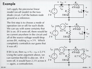
13. EE 201 diodes – 13
Although the non-linear nature of the diode caused some mathematical
difficulties requiring numerical techniques, the analysis wasn’t really that
bad. In fact, the iteration technique was sort of interesting.
However, the difficulty escalates
quickly when circuits become just a
little bit more complicated.
Consider the circuit at right — it
doesn’t look that bad.
Try node voltage (ground at the bottom, two node voltages vR1 and vD2):
iD1 = iR1 + iR2 =
vR1
R1
+
vR1 − vD2
R2
iD2 =
vR1 − vD2
R2
+
–
VS
3 V
iD2
–
+
vD2
470 kΩ
R1
330 Ω
R2
–
+ vD1
iD1
IS1
[
exp
(
vD1
kT/q)
− 1
]
= IS1
[
exp
(
VS − vR1
kT/q )
− 1
]
=
vR1
R1
+
vR1 − vD2
R2
IS2
[
exp
(
vD2
kT/q)
− 1
]
=
vR1
R1
+
vR1 − vD2
R2
Two unknowns, related by two non-linear equations! Not good.

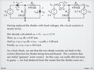
14. EE 201 diodes – 14
+
–
VS
3 V
iD2
–
+
vD2
470 kΩ
R1
330 Ω
R2
–
+ vD1
iD1
Maybe mesh currents would be
better. We can relate the two
currents iD1 and iD2.
VS − vD1 − vR1 = 0
vR1 − vR2 − vD2 = 0
VS − vD1 − R1 (iD1 − iD2) = 0
R1 (iD1 − iD2) − R2iD2 − vD2 = 0
VS −
kT
q
ln
[
iD1
IS1
+ 1
]
− R1 (iD1 − iD2) = 0
R1 (iD1 − iD2) − R2iD2 −
kT
q
ln
[
iD2
IS2
+ 1
]
= 0
Still two non-linear equations relating the two unknowns. There is no
way around it. No other techniques are even applicable — no such
thing as equivalent diodes, diode dividers, or diode transformations.
Our best option is to look for some sort of short-cut.

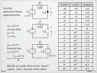
15. EE 201 diodes – 15
VS (V) vD (V) iD (mA)
–10 –10 ≈ 0
–8 –8 ≈ 0
–6 –6 ≈ 0
–4 –4 ≈ 0
–2 –2 ≈ 0
0 0 0
1
v
0.628 0.372
2 0.661 1.339
3 0.675 2.325
4
v
0.684 3.316
5 0.691 4.309
6 0.697 5.304
7 0.701 6.299
8 0.705 7.295
9 0.708 8.292
10 0.711 9.289
When the diode is reverse-biased
(VS < 0, so vD < 0), it behaves
essentially like an open circuit, iD ≈ 0.
When the diode is forward-biased
(VS > 0, so vD > 0), its voltage is
approximately the same in each
case, vD ≈ 0.7 V.
+
–
VS
1.5 V
iD
–
+
vD
R
1 kΩ
Return to the earlier single-diode
example. Solve for iD and vD
exactly for a range of VS values.
iD =
VS
R
−
kT/q
R
ln
[
iD
IS
+ 1
]

16. EE 201 diodes – 16
piecewise diode model
The results of the previous slide suggest an approximation:
• When reverse-biased, we treat the diode as if it is an open-circuit.
• When forward-biased, we treat it like an ideal source with a value
of 0.7 V.
–
vD
> 0
+
iD
+
– 0.7 V
iD
Reverse (vD < 0.7 V) Forward (vD = 0.7 V)
Note that the diode is NOT a
voltage source. It is a passive
device and does not provide
power to the circuit. But it does
behave as if it were a voltage
source or battery that is absorbing
power.
To use the models.
• Guess forward or reverse
• Insert the corresponding model
• Solve for voltage/current using model
• Check the result: for reverse, vD < 0, for
forward, iD flows in correct direction
–
vD
< 0.7 V
+
iD
= 0
–
vD
+
iD
= 0

17. EE 201 diodes – 17
VS (V) vD (V) iD (mA)
–10 –10 ≈ 0
–8 –8 ≈ 0
–6 –6 ≈ 0
–4 –4 ≈ 0
–2 –2 ≈ 0
0 0 0
1
v
0.7 0.3
2 0.7 1.3
3 0.7 2.3
4
v
0.7 3.3
5 0.7 4.3
6 0.7 5.3
7 0.7 6.3
8 0.7 7.3
9 0.7 8.3
10 0.7 9.3
VS < 0.7 V:
reverse bias.
iD = 0.
vD = VS.
Results are quite close to the “exact”
values, with a fraction of the effort.
+
–
VS
1.5 V
iD
–
+
vD
R
1 kΩ
Use the
piecewise-linear
approximation.
+
–
VS iD
–
+
vD
R
1 kΩ
+
–
VS iD
0.7 V
R
1 kΩ
+
–
VS > 0.7 V:
forward bias.
vD = 0.7 V.
iD =
VS − 0.7 V
R

18. EE 201 diodes – 18
Example
Let’s apply the piecewise linear
model (on-off model) to the two-
diode circuit. Call the bottom node
ground as a reference.
The first step is to choose a mode of
operation (on or off) for each diode.
We can say with some certainty that
D1 is on. (If it were off, there would be
no current anywhere in the circuit and
all of the source voltage would drop
across D1, making vD1 = 3 V. Which
completely contradicts our guess that
it was off.)
If D1 is on, then vR1 = VS – vD1 = 2.3 V.
Using the same argument above, we
can surmise that D2 is also on. (If it
were off, it would have 2.3 V across it
— again, a contradiction.
+
–
VS
3 V
iD2
–
+
vD2
470 kΩ
R1
330 Ω
R2
–
+ vD1
iD1
+
–
VS
3 V
iD2
–
+
vD2
470 kΩ
R1
330 Ω
R2
vD1
iD1
+
–
0.7 V
+
–
VS
3 V
iD2
vD2
470 kΩ
R1
330 Ω
R2
vD1
iD1
+
–
0.7 V +
–
0.7 V

19. EE 201 diodes – 19
+
–
VS
3 V
iD2
–
+
vD2
470 kΩ
R1
330 Ω
R2
–
+ vD1
iD1 +
–
VS
3 V
iD2
vD2
470 kΩ
R1
330 Ω
R2
vD1
iD1
+
–
0.7 V +
–
0.7 V
Having replaced the diodes with fixed voltages, the circuit analysis is
nearly trivial.
We already calculated vR1 = VS – vD1 = 2.3 V.
Then, iR1 = vR1 /R1 = 6.97 mA.
And iD2 = iR2 = vR2 /R1 = (vR1 – vD2)/R2 = 3.40 mA.
Finally, iD1 = iR1 + iD2 = 10.4 mA
As a final check, we see that the two diode currents are both in the
correct direction for diodes being forward-biased. This confirms that
our initial “guesses” were correct. (In this case, we really did not have
to guess — we had deduced from the outset that the diodes were on.)