Diffusion Quantum Theory And Radically Elementary Mathematics Mn47 William G Faris
Diffusion Quantum Theory And Radically Elementary Mathematics Mn47 William G Faris
Diffusion Quantum Theory And Radically Elementary Mathematics Mn47 William G Faris
Diffusion Quantum Theory And Radically Elementary Mathematics Mn47 William G Faris
Diffusion Quantum Theory And Radically Elementary Mathematics Mn47 William G Faris
1.
Diffusion Quantum TheoryAnd Radically
Elementary Mathematics Mn47 William G Faris
download
https://ebookbell.com/product/diffusion-quantum-theory-and-
radically-elementary-mathematics-mn47-william-g-faris-34750098
Explore and download more ebooks at ebookbell.com
2.
Here are somerecommended products that we believe you will be
interested in. You can click the link to download.
Diffusion Quantum Theory And Radically Elementary Mathematics Mn47
William G Faris Editor
https://ebookbell.com/product/diffusion-quantum-theory-and-radically-
elementary-mathematics-mn47-william-g-faris-editor-51945024
Diffusion Quantum Theory And Radically Elementary Mathematics William
G Faris
https://ebookbell.com/product/diffusion-quantum-theory-and-radically-
elementary-mathematics-william-g-faris-4986090
Quantum State Diffusion Ian Percival
https://ebookbell.com/product/quantum-state-diffusion-ian-
percival-1861642
Quantum Trajectories And Measurements In Continuous Time The Diffusive
Case 1st Edition Alberto Barchielli
https://ebookbell.com/product/quantum-trajectories-and-measurements-
in-continuous-time-the-diffusive-case-1st-edition-alberto-
barchielli-1149404
3.
Diffusion Tensor ImagingAnd Fractional Anisotropy Imaging Biomarkers
In Early Parkinsons Disease Rahul P Kotian
https://ebookbell.com/product/diffusion-tensor-imaging-and-fractional-
anisotropy-imaging-biomarkers-in-early-parkinsons-disease-rahul-p-
kotian-47136552
Diffusion Under The Effect Of Lorentz Force Erik Kalz
https://ebookbell.com/product/diffusion-under-the-effect-of-lorentz-
force-erik-kalz-47217506
Diffusion Of Democracy The Past And Future Of Global Democracy Barbara
Wejnert
https://ebookbell.com/product/diffusion-of-democracy-the-past-and-
future-of-global-democracy-barbara-wejnert-47505924
Diffusion In Minerals And Melts Youxue Zahng Editor Daniele J Cherniak
Editor
https://ebookbell.com/product/diffusion-in-minerals-and-melts-youxue-
zahng-editor-daniele-j-cherniak-editor-50924108
Diffusion Segregation And Solidstate Phase Transformations Course
Reminders And Solved Problems Didier Blavette Thomas Philippe
https://ebookbell.com/product/diffusion-segregation-and-solidstate-
phase-transformations-course-reminders-and-solved-problems-didier-
blavette-thomas-philippe-51812226
Diffusion, Quantum Theory,and
Radically Elementary
Mathematics
Mathematical Notes 47
edited by William G. Faris
PRINCETON UNIVERSITY PRESS
PRINCETON AND OXFORD
9.
Copyright c 2006by Princeton University Press
Published by Princeton University Press,
41 William Street, Princeton, New Jersey 08540
In the United Kingdom: Princeton University Press,
3 Market Place, Woodstock, Oxfordshire 0X20 1SY
All Rights Reserved
Library of Congress Control Number 2006040533
ISBN-13: 978-0-691-12545-9 (pbk. : alk. paper)
ISBN-10: 0-691-12545-7 (pbk. : alk. paper)
British Library Cataloging-in-Publication Data is available.
The publisher would like to acknowledge the author of this volume
for providing the camera-ready copy from which this book was printed.
This book has been composed in Times Roman using L
A
TEX.
Printed on acid-free paper. ∞
pup.princeton.edu
Printed in the United States of America
10 9 8 7 6 5 4 3 2 1
10.
The Laplace operatorin its various manifestations is the most
beautiful and central object in all of mathematics. Probability
theory, mathematical physics, Fourier analysis, partial differen-
tial equations, the theory of Lie groups, and differential geome-
try all revolve around this sun, and its light even penetrates such
obscure regions as number theory and algebraic geometry.
Edward Nelson, Tensor Analysis
Contents
Preface ix
Chapter 1.Introduction: Diffusive Motion and Where It Leads
William G. Faris 1
Chapter 2. Hypercontractivity, Logarithmic Sobolev Inequalities,
and Applications: A Survey of Surveys
Leonard Gross 45
Chapter 3. Ed Nelson’s Work in Quantum Theory
Barry Simon 75
Chapter 4. Symanzik, Nelson, and Self-Avoiding Walk
David C. Brydges 95
Chapter 5. Stochastic Mechanics: A Look Back and a Look Ahead
Eric Carlen 117
Chapter 6. Current Trends in Optimal Transportation:
A Tribute to Ed Nelson
Cédric Villani 141
Chapter 7. Internal Set Theory and Infinitesimal Random Walks
Gregory F. Lawler 157
Chapter 8. Nelson’s Work on Logic and Foundations
and Other Reflections on the Foundations of Mathematics
Samuel R. Buss 183
Chapter 9. Some Musical Groups:
Selected Applications of Group Theory in Music
Julian Hook 209
Chapter 10. Afterword
Edward Nelson 229
Preface
Diffusive motion—displacement dueto the cumulative effect of irregular
fluctuations—has been a fundamental concept in mathematics and physics since
the work of Einstein on Brownian motion. It is also relevant to understanding vari-
ous aspects of quantum theory. This volume explains diffusive motion and its rela-
tion to both nonrelativistic quantum theory and quantum field theory. It also shows
how diffusive motion concepts lead to a radical reexamination of the structure of
mathematical analysis.
Einstein’s original work on diffusion was already remarkable. He suggested a
probability model describing a particle moving along a path in such a way that it
has a definite position at each instant, but with a motion so irregular that it has
no well-defined velocity. Since the main tool of a physicist is the relation between
force and rate of change of velocity, it was astonishing that he could dispense with
velocity and still make predictions about Brownian motion. The story of how he
did this is told in Edward Nelson’s Dynamical Theories of Brownian Motion. In
brief, Einstein worked with an average velocity, or drift, defined in a subtle way
by ignoring the irregular fluctuations. In his analysis this average velocity results
from a balance of external force and frictional force. The external force might be
gravity, but, as Nelson remarks, the beauty of the argument is that this force is
entirely virtual. In other words, it only has to be nonzero, and it does not appear in
Einstein’s final result for the diffusion coefficient.
Diffusion is part of probability theory, while quantum mechanics involves waves
with complex number amplitudes. However, diffusion is related to quantum me-
chanics in various ways. The Wiener integral over paths that underlies the Einstein
model for Brownian motion has a complex number analog in the Feynman path in-
tegral of quantum mechanics. While the properties of the Feynman path integral are
elusive, the probability models that describe diffusion are precise mathematical ob-
jects, and they have direct connections to quantum mechanics. These connections
form a thread that runs through this book.
The introductory chapter by Faris describes the interrelationships between the
book’s various themes, many of which were first brought to light by Nelson. One
major theme is Markovian diffusion, where a particle wanders randomly but also
feels the influence of systematic drift. Diffusion is related to quantum theory and
quantum field theory in several ways. These connections, both technical and con-
ceptual, are particularly apparent in the chapters by Gross, Simon, Brydges, Carlen,
and Villani.
Another important theme is the need for a closer look at the irregular paths aris-
ing from the diffusion. Intuitively they each consist of an unlimited number of
15.
x PREFACE
infinitesimal randomsteps. Lawler’s chapter makes this notion precise by using a
syntactic approach to nonstandard analysis. This approach employs an augmented
language that recognizes among the real numbers some that are infinitesimal and
some that are unlimited in size. When this framework is applied to natural numbers,
it happens that among the natural numbers there are some that are unlimited, that
is, greater than each standard natural number. Furthermore, one way of describing
a diffusion process is in terms of a finite sequence of random variables, where the
number of variables, while finite, is unlimited in just this sense.
This leads to a related topic, the syntactic description of natural numbers, which
is explored in the chapter by Sam Buss. A final chapter explores the mathematical
structure of musical composition, which turns out to parallel the structure of space-
time. This contribution is by Jay Hook, who was a Ph.D. student of Nelson in
mathematics before turning to music theory.
The idea for this book came out of the conference Analysis, Probability, and
Logic, held at the Mathematics Department of the University of British Columbia
on June 17 and 18, 2004. It was in honor of Edward Nelson, professor at Princeton
University, who has done beautiful and influential work in probability, functional
analysis, mathematical physics, nonstandard analysis, stochastic mechanics, and
logic.
The conference was hosted and supported by the Pacific Institute of Mathemat-
ical Sciences (PIMS). The National Science Foundation (USA) provided travel
support for some participants. The organizers were David Brydges, Eric Carlen,
William Faris, and Greg Lawler. The presentations at this conference led to the
present volume. The editor thanks all who provided help with its preparation, in-
cluding the authors, William Priestly, and Joseph McMahon. He is also grateful to
the editors at Princeton University Press, Vickie Kearn and Linny Schenck, and to
the copyeditor, Beth Gallagher, who gave generously of their expertise.
16.
Chapter One
Introduction: DiffusiveMotion and Where It Leads
William G. Faris∗
1.1 DIFFUSION
The purpose of this introductory chapter is to point out the unity in the following
chapters. At first this might seem a difficult enterprise. The authors of these chap-
ters treat diffusion theory, quantum mechanics, and quantum field theory, as well
as stochastic mechanics, a variant of quantum mechanics based on diffusion ideas.
The contributions also include an infinitesimal approach to diffusion and related
probability topics, an approach that is radically elementary in the sense that it relies
only on simple logical principles. There is further discussion of foundational prob-
lems, and there is a final essay on the mathematics of music. What could these have
in common, other than that they are in some way connected to the work of Edward
Nelson?
In fact, there are important links between these topics, with the apparent excep-
tion of the chapter on music. However, the chapter on music is so illuminating, at
least to those with some acquaintance with classical music, that it alone may attract
many people to this collection. In fact, there is an unexpected connection to the
other topics, as will become apparent in the following more detailed discussion.
The plan is to begin with diffusion and then see where this leads.
In ordinary free motion distance is proportional to time:
∆x = v∆t. (1.1)
This is sometimes called ballistic motion. Another kind of motion is diffusive mo-
tion. The characteristic feature of diffusion is that the motion is random, and dis-
tance is proportional to the square root of time:
∆x = ±σ
√
∆t. (1.2)
As a consequence diffusive motion is irregular and inefficient. The mathematics of
diffusive motion in explained in sections 1.1–1.3 of this chapter.
There is a close but subtle relation between diffusion and quantum theory. The
characteristic indication of quantum phenomena is the occurrence of the Planck
constant ~ in the description. This constant has the dimensions ML2
/T of angular
momentum. The relation to diffusion derives from
σ2
=
~
m
, (1.3)
∗Department of Mathematics, University of Arizona, Tucson, AZ 85721, USA
17.
2 CHAPTER 1
wherem is the mass of the particle in the quantum system. The diffusion constant
σ2
has the appropriate dimensions L2
/T for a diffusion; that is, it characterizes a
kind of motion where distance squared is proportional to time.
In quantum mechanics it is customary to define the dynamics by quantities ex-
pressed in energy units, that is, with dimensions ML2
/T2
. The determination of
the time dynamics involves a division by ~, which changes the units to inverse time
units 1/T. In the following exposition energy quantities, such as the potential en-
ergy function V (x), will be in inverse time units. This should make the comparison
with diffusion theory more transparent.
One connection between quantum theory and diffusion is the relationship be-
tween real time in one theory and imaginary time in the other theory. This connec-
tion is precise and useful, both in the quantum mechanics of nonrelativistic particles
and in quantum field theory. This connection is explored in sections 1.4–1.7.
The marriage of quantum theory and the special relativity theory of Einstein and
Minkowski is through quantum field theory. In relativity theory a mass m has an
associated momentum mc and an associated energy mc2
. These define in turn a
spatial decay rate
mL =
mc
~
(1.4)
and a time decay rate
mT =
mc2
~
. (1.5)
These set the distance and time scales for quantum fluctuations in relativistic field
theory. This theory is related to diffusion in an infinite-dimensional space of Eu-
clidean fields. Some features of this story are explained in sections 1.8–1.10 of this
introduction and in the later chapters by Leonard Gross, Barry Simon, and David
Brydges.
The passage from real time to imaginary time is convenient but artificial. How-
ever, in the domain of nonrelativistic quantum mechanics of particles there is a
closer connection between diffusion theory and quantum theory. In stochastic me-
chanics the real time of quantum mechanics is also the real time of diffusion, and in
fact quantum mechanics itself is formulated as conservative diffusion. This subject
is sketched in sections 1.11–1.12 of this introduction and in the chapters by Eric
Carlen and Cédric Villani.
The conceptual importance of diffusion leads naturally to a closer look at math-
ematical foundations. In the calculus of Newton and Leibniz, motion on short time
and distance scales looks like ballistic motion. This is not true for diffusive motion.
On short time and distance scales it looks like the Wiener process, that is, like the
Einstein model of Brownian motion. In fact, there are two kinds of calculus for
the two kinds of motion, the calculus of Newton and Leibniz for ballistic motion
and the calculus of Itô for diffusive motion. The calculus of Newton and Leibniz
in its modern form makes use of the concept of limit, and the calculus of Itô relies
on limits and on the measure theory framework for probability. However, there is
another calculus that can describe either kind of motion and is quite elementary.
This is the infinitesimal calculus of Abraham Robinson, where one interprets ∆t
18.
INTRODUCTION 3
and ∆xas infinitesimal real numbers. It may be that this calculus is particularly
suitable for diffusive motion. This idea provides the theme in sections 1.13–1.14 of
this introduction and leads to the later contributions by Greg Lawler and Sam Buss.
The concluding section 1.15 connects earlier themes with a variation on musical
composition, presented in the final chapter by Julian Hook.
1.2 THE WIENER WALK
The Wiener walk is a mathematical object that is transitional between random walk
and the Wiener process. Here is the construction of the appropriate simple sym-
metric random walk. Let ξ1, . . . , ξn be a finite sequence of independent random
variables, each having the values ±1 with equal probability. One way to construct
such random variables is to take the set {−1, 1}n
of all sequences ξ of n values
±1 and give it the uniform probability measure. Then ξk is the kth element in the
sequence, and the function ξ 7→ ξk is the corresponding random variable. The ran-
dom walk is the sequence sk = ξ1 +· · ·+ξk defined for 0 ≤ k ≤ n. The underlying
probability space in this construction is finite, with 2n
points.
Here is the construction of the n-step Wiener walk on the time interval [0, T].
Let ∆t = T/n be the time step. Fix the diffusion constant σ2
> 0, and let the
corresponding space step be
∆x = σ
√
∆t. (1.6)
If
tk = k∆t (1.7)
for k = 0, 1, 2, . . . n, define
wn
(tk) = ξ1∆x + · · · + ξk∆x. (1.8)
Finally, define w(n)
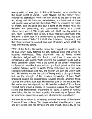
(t) for real t with 0 ≤ t ≤ T by linear interpolation. Then
w(n)
is a random real continuous function defined on [0, T]. This random function
is the Wiener walk with time step ∆t = T/n. A typical sample path is illustrated
in Figure 1.1.
Let C([0, T]) be the metric space of all real continuous functions on the time
interval [0, T]. Let µ(n)
be the probability measure induced on Borel subsets of
C([0, T]) by the random function w(n)
. That is, the probability of a Borel subset
is the probability that the function w(n)
is in this subset. This probability measure
µ(n)
is the distribution of the Wiener walk. It is concentrated on a finite set of 2n
piecewise linear continuous paths.
1.3 THE WIENER PROCESS
The Wiener process is a fundamental object in probability theory, describing a par-
ticular kind of random path. Another common name for it is Brownian motion,
since it is closely related to the Einstein model for Brownian motion of a physical
19.
4 CHAPTER 1
1020 30 40 50
t
-8
-6
-4
-2
2
x
Figure 1.1 A sample path of the Wiener walk.
particle. There are other models of the physical process of Brownian motion, so it
is clearer to use “Wiener process” for the mathematical object.
The Wiener process may be constructed in a number of ways, but one way to
get an intuition for it is to think of it as a limit of the Wiener walk. In this limit the
distribution of the Wiener walk, which is given by binomial probabilities, converges
to the distribution of the Wiener process, which is Gaussian.
PROPOSITION 1.1 (Construction of Wiener measure) For each n = 1, 2, 3, . . .
let µ(n)
be the probability measure defined on Borel subsets of C([0, T]) defined by
the Wiener walk with time step ∆t satisfying n∆t = T. Then there is a probability
measure µ defined on the Borel subsets of C([0, T]) such that µ(n)
→ µ as n → ∞
in the sense of weak convergence of probability measures.
This result may be found in texts on probability [2]. The statement about weak
convergence means that for each bounded continuous real function F defined on
the space C([0, T]) the expectation
R
F dµ(n)
→
R
F dµ as n → ∞. This µ is the
Wiener measure with diffusion parameter σ2
. If t is fixed, then the map w 7→ w(t)
is a function from the probability space C([0, T]) with Wiener measure µ to the real
numbers, and hence is a random variable. For each t ≥ 0 this random variable w(t)
has mean zero and variance σ2
t. Furthermore, the increments of w corresponding
to disjoint time intervals are independent. Since the random variable w(t) is the
sum of an arbitrarily large number of independent increments, by the central limit
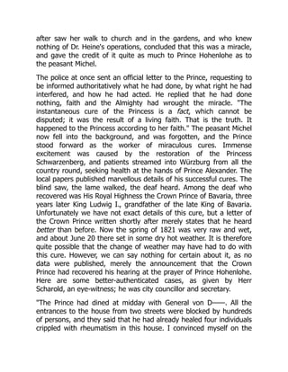
theorem it must have a Gaussian distribution. The random continuous function w
associated with the Wiener measure is the Wiener process. A typical sample path
is sketched in Figure 1.2.
So far the Wiener process has been defined as a random continuous function
on a bounded interval [0, T] of time. However, it is not difficult to build the un-
bounded interval [0, +∞) out of a sequence of bounded intervals and thus give a
20.
INTRODUCTION 5
10 2030 40 50
t
-0.6
-0.4
-0.2
0.2
0.4
x
Figure 1.2 A sample path of the Wiener process.
definition of the Wiener process as a random continuous function on this larger
time interval. In fact, it is even possible to define the Wiener process for the time
interval (−∞, +∞) as a random continuous function satisfying the normaliza-
tion w(0) = 0. Henceforth the Wiener process will refer to the probability space
C((−∞, +∞)) with the probability measure µ defined in this way.
In the following the expectation of a random variable F defined on the space
C((−∞, +∞)) with respect to the Wiener measure µ is written
µ[F] =
Z
F dµ. (1.9)
That is, the same notation is used for expectation as for probability. For example,
the expectation of w(t) (as a function of w) is µ[w(t)] = 0, and the variance is
µ[w(t)2
] = σ2
|t|.
Another useful topic is weighted increments of the Wiener process and the cor-
responding Wiener stochastic integral. Let t1 < t2, and consider the corresponding
increment w(t2) − w(t1). This is Gaussian with mean zero and variance σ2
(t2 −
t1) = σ2
|[t1, t2]|, which is proportional to the length of the interval. Consider two
such increments w(t2) − w(t1) and w(t′
2) − w(t′
1). The condition of independent
increments implies that they have covariance
µ[(w(t2) − w(t1))(w(t′
2) − w(t′
1))] = σ2
|[t1, t2] ∩ [t′
1, t′
2]|, (1.10)
which is proportional to the length of the intersection of the two intervals.
This generalizes to weighted increments. Let f be a real function such that
R ∞
−∞
f(t)2
dt < +∞. Then the Wiener stochastic integral
R ∞
−∞
f(t)d w(t) is a
well-defined Gaussian random variable with mean zero. Furthermore, the condi-
tion of independent increments implies that the covariance of two such stochastic
integrals is
µ
Z ∞
−∞
f(t) dw(t)
Z ∞
−∞
g(t′
) dw(t′
)
= σ2
Z ∞
−∞
f(t)g(t) dt. (1.11)
21.
6 CHAPTER 1
Theindependent increment property (1.10) is the special case when f and g are
indicator functions of intervals.
Another description of the Wiener process is by a partial differential equation.
For t 0 let ρ(y, t) (as a function of y) be the probability density of the Wiener
process at time t, so that
µ[f(w(t))] =
Z ∞
−∞
f(y)ρ(y, t) dy. (1.12)
Since the density ρ(y, t) is Gaussian with mean zero and variance σ2
t, it follows
that it satisfies the partial differential equation
∂ρ
∂t
=
1
2
σ2 ∂2
ρ
∂y2
. (1.13)
This is the simplest diffusion equation (or heat equation).
For a Wiener process describing diffusion in finite-dimensional Euclidean space
the probability density is jointly Gaussian. There is also a corresponding partial
differential equation, in which the second derivative in the space variable is replaced
by the Laplace operator.
Later it will appear that in infinite-dimensional space it is preferable to deal with
the Ornstein–Uhlenbeck velocity process instead of the Wiener process. The proba-
bility distributions are jointly Gaussian, but they have a more complicated time de-
pendence. They still solve a second-order linear partial differential equation. How-
ever, this equation involves the sum of the Laplace operator with another operator,
the first-order differential along the direction of a linear vector field.
1.4 DIFFUSION, KILLING, AND QUANTUM MECHANICS
The first remarkable discovery connecting quantum mechanics with diffusion the-
ory is that the fundamental equation of quantum mechanics is closely related to
an equation describing diffusion with killing. As we shall see, the connection is
through the Feynman–Kac formula.
Quantum theory, of course, is the ultimate mystery of modern science. It has
many strange features, such as remarkable correlations over long distances. These
correlations are experimentally observed, and their peculiar nature takes mathe-
matical shape in the form of a violation of Bell’s inequalities. The appendix to [17]
gives an account of this subject and its implications.
However strange quantum mechanics may be, there is universal agreement that
the wave function ψ for an isolated system satisfies the Schrödinger equation
∂ψ
∂t
= i
1
2
σ2 ∂2
∂x2
− V (x)
ψ. (1.14)
Here σ2
= ~/m and V (x) is the potential energy, here measured in inverse time
units.
This is often stated in terms of the Schrödinger operator H defined by
H = −
1
2
σ2 ∂2
∂x2
+ V (x). (1.15)
22.
INTRODUCTION 7
-3 -2-1 1 2 3
x
-0.5
0.5
1
1.5
rate
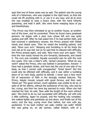
Figure 1.3 A killing rate (potential) function with subtraction V (x) − λ0.
Then the Schrödinger equation (1.14) has the form
∂ψ
∂t
= −iHψ. (1.16)
This way of writing the equation differs slightly from the usual quantum mechan-
ical convention. The usual quantum mechanical potential energy and total energy
are obtained from the V and H in the present treatment by multiplication by the
constant ~. This converts inverse time units to energy units. In quantum mechanics
the dynamics is defined by dividing energy by ~, therefore returning to inverse time
units. So in the present notation, with inverse time units for H, the solution of the
Schrödinger equation with initial condition ψ(x) = ψ(x, 0) is
ψ(x, t) = (e−itH
ψ)(x). (1.17)
This operator exponential may be interpreted via spectral theory or by the theory
of one-parameter semigroups [9].
There are several connections between quantum mechanics and diffusion. The
most obvious ones are treated here in sections 1.4–1.7. There is also a more pro-
found connection between the Schrödinger equation and diffusion given by the
equations of stochastic mechanics. That will be the subject of sections 1.11–1.12.
A particularly simple way to go from quantum mechanics to diffusion is to re-
place it by t. The resulting diffusion equation is then
∂r
∂t
=
1
2
σ2 ∂2
∂x2
− V (x)
r. (1.18)
Here σ2
is interpreted as a diffusion constant. The diffusing particle randomly van-
ishes at a certain rate V (x) ≥ 0 depending on its position x in space. Thus there is
some chance that at a random time τ it will cease to diffuse and vanish. In proba-
bility it is common to say that the particle is killed. A typical killing rate function
V (x) is sketched in Figure 1.3. Actually, the sketch shows V (x) − λ0, where the
subtracted constant λ0 is the least eigenvalue of H.
The solution r(x, t) has a probability interpretation. Let r(y) be a given function
of the position variable y. Then r(x, t) is the expectation of r(y), when y is taken
23.
8 CHAPTER 1
asthe random position of the diffusing particle at time t ≥ 0, provided that the
particle was started at x at time 0 and has not yet vanished. (The contribution to the
expected value for a particle that has vanished is zero.) The initial condition for the
equation is r(x, 0) = r(x). The equation
∂r
∂t
= −Hr (1.19)
has an operator solution, this time of the form
r(x, t) = (e−tH
r)(x). (1.20)
This operator exponential may also be interpreted via spectral theory or by the
theory of one-parameter semigroups. However, in this case there is also a direct
probabilistic solution of equation (1.18) given by the Feynman–Kac formula.
PROPOSITION 1.2 (Diffusion with killing: The Feynman–Kac formula) The so-
lution of the equation for diffusion with killing is given by
r(x, t) = µ
h
e−
R t
0
V (x+w(s)) ds
r(x + w(t))
i
. (1.21)
This says that the solution is obtained by letting the particle diffuse according to
a Wiener process, but with a chance to vanish from its current location in space at
a rate proportional to the value of V at this location. The exponential factor is the
probability that the particle has not yet vanished at time t. There are discussions of
the Feynman–Kac formula in Nelson’s article [6] on the Feynman integral and in
the book by Simon [16] on functional integration.
1.5 DIFFUSION, DRIFT, AND QUANTUM MECHANICS
Another connection of quantum mechanics with diffusion is more subtle. Instead
of diffusion with killing, there is diffusion with a drift that maintains equilibrium.
Let H be the Schrödinger operator (1.15) of section 1.4, expressed as before
in inverse time units. Suppose that H has an an eigenfunction ψ0(x) 0 with
eigenvalue λ0. Thus
−
1
2
σ2 ∂2
∂x2
+ V (x)
ψ0 = λ0ψ0. (1.22)
This gives a particular decay mode solution of the diffusion with killing equa-
tion (1.18) of the form r0(x, t) = e−λ0t
ψ0(x).
The interpretation in terms of diffusion with drift comes from the change of
variable r(x, t) = f(x, t)e−λ0t
ψ0(x). In other words, f(x, t) is the ratio of the
solution to the decay mode solution, which is seen to satisfy the partial differential
equation
∂f
∂t
=
1
2
σ2 ∂2
∂x2
+ u(x)
∂
∂x
f. (1.23)
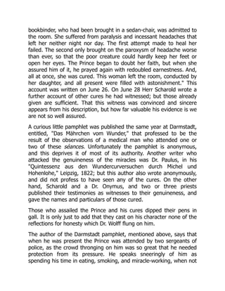
Here the function u(x) represents a drift vector field given by
u(x) = σ2 1
ψ0(x)
∂ψ0(x)
∂x
. (1.24)
24.
INTRODUCTION 9
-3 -2-1 1 2 3
x
-0.6
-0.4
-0.2
0.2
0.4
0.6
drift
Figure 1.4 A drift function u(x).
A typical drift function u(x) is sketched in Figure 1.4.
Again this equation has an operator solution. Define the backward diffusion with
drift operator Ĥ by a similarity transformation given by the operator product
Ĥ =
1
ψ0
· (H − λ0) · ψ0. (1.25)
The transformed operator has the form
Ĥ = −
1
2
σ2 ∂2
∂x2
− u(x)
∂
∂x
. (1.26)
The first term is the diffusion term, and the second term is the term corresponding
to a drift u(x).
The equation (1.23) may be written as the backward equation
∂f
∂t
= −Ĥf. (1.27)
A particle starts at x and diffuses under the influence of the drift. Let f(y) be a given
function of the position variable y. Then the solution f(x, t) is the expectation of
f(y), where y is taken as the random position of the diffusing particle at time
t ≥ 0, provided that the particle was started at x at time 0. The initial condition for
the equation is f(x, 0) = f(x). The operator solution of this equation is given by
f(x, t) = (e−tĤ
f)(x). (1.28)
One probabilistic solution arises from the Feynman–Kac formula (1.21), given
by
f(x, t) = eλ0t
µ
1
ψ0(x)
e−
R t
0
V (x+w(s)) ds
f(x + w(t))ψ0(x + w(t))
. (1.29)
However, this solution emphasizes the connection with killing. The true nature of
this solution is revealed by looking at it directly as a diffusion process with drift
vector field u(x).
The diffusion process with drift u may be defined directly by the stochastic dif-
ferential equation
dx(t) = u(x(t)) dt + dw(t). (1.30)
25.
10 CHAPTER 1
withthe initial condition x(0) = x. The first term on the right represents the effect
of the systematic drift, while the second term on the right represents the influ-
ence of random diffusion. This equation involves the Wiener path, which is non-
differentiable with probability 1. However it may be formulated in integrated form
as
x(t) − x =
Z t
0
u(x(s)) ds + w(t). (1.31)
For each continuous path w(t) this equation determines a corresponding continuous
path x(t). Since the w(t) paths are random (given by the Wiener process), the x(t)
paths are also random. In particular, let f(y) be a function of the space variable,
and consider the expectation
f(x, t) = µ[f(x(t)) | x(0) = x] (1.32)
as a function of time and the starting position.
PROPOSITION 1.3 (Diffusion with drift: Stochastic differential equation) Sup-
pose the diffusion with drift process x(t) is defined by the stochastic differential
equation with the initial condition x(0) = x. Then the expectation f(x, t) satisfies
the backward diffusion with drift equation.
In other words, the expectation satisfies equation (1.23). This result is standard in
the theory of Markov diffusion processes. A charming account is found in Nelson’s
book [7].
1.6 STATIONARY DIFFUSION
Another way of describing diffusion with drift is in terms of probability density.
Say that instead of starting the diffusing particle at a fixed point, its starting point is
random with probability density ρ(x). Then, after time t, the probability will have
diffused to ρ(y, t). Thus, if one computes the expectation of a function f(y) of the
position at time t, one gets
Z ∞
−∞
f(y)ρ(y, t) dy =
Z ∞
−∞
f(x, t)ρ(x) dx. (1.33)
The density satisfies a partial differential equation, the forward equation (or
Fokker–Planck equation). It is
∂ρ
∂t
=
1
2
σ2 ∂2
∂y2
−
∂
∂y
u(y)
ρ. (1.34)
Again this has an operator form. Define the forward diffusion with drift operator
Ĥ′
by another similarity transformation, this time given by the operator product
Ĥ′
= ψ0 · (H − λ0) ·
1
ψ0
. (1.35)
This has the form
Ĥ′
= −
∂
∂y
1
2
σ2 ∂
∂y
− u(y)
. (1.36)
26.
INTRODUCTION 11
-3 -2-1 1 2 3
x
0.1
0.2
0.3
0.4
0.5
density
Figure 1.5 A stationary density ρ0(x).
The equation
∂ρ
∂t
= −Ĥ′
ρ (1.37)
has an operator solution
ρ(y, t) = (e−tĤ′
ρ)(y). (1.38)
Let
ρ0(x) = ψ0(x)2
. (1.39)
Then ρ0 is interpreted as an equilibrium probability density. The drift u may be
expressed directly in terms of ρ0 by
u(x) =
1
2
σ2 1
ρ0(x)
∂ρ0(x)
∂x
. (1.40)
Say that the initial probability density ρ(x) = ρ0(x), the probability density that
defines the diffusion process. Then since Ĥ′
ρ0 = 0 the density remains the same;
that is, ρ(x, t) = ρ0(x) for all t. This is the stationary diffusion process. A typical
stationary density is shown in Figure 1.5.
Since the stationary diffusion process is defined from the process with killing
by a similarity transformation, the measure associated with the stationary diffusion
process may be defined in terms of the killing rate V (y) by
µ̂[F] = eT λ0
Z
ρ0(x)µ
F
1
ψ0(x)
e−
R T
0
V (x+w(s)) ds
ψ0(x + w(T))
dx. (1.41)
Here F depends on the path x(s) for s between time 0 and time T. Since ρ0(x) =
ψ0(x)2
this is equivalent to
µ̂[F] = eT λ0
Z
µ[Fψ0(x)e−
R T
0
V (x+w(s)) ds
ψ0(x + w(T))] dx. (1.42)
This suggests that it should be possible to construct the stationary diffusion with
drift measure directly from the Wiener measure with killing, without using the
27.
12 CHAPTER 1
1020 30 40 50
t
-2
-1
1
2
x
Figure 1.6 A sample path of a nonlinear diffusion dx = u(x) dt + dw(t).
knowledge of the ground state wave function ψ0(x). This sort of construction turns
out to be useful in the field theory context discussed in sections 1.8–1.10. Let
µ̂T [F] =
1
ZT
µ[Fe−
R T
0
V (w(s)) ds
δ(w(T))]. (1.43)
This is the Wiener expectation, conditioned on returning to 0 after time T and on
not vanishing. The delta function enforces the condition of return to the origin,
and the ZT in the denominator is the probability of not vanishing along the way.
Suppose that T is large and that F depends only on part of the path well in the
interior of the interval from 0 to T. The expectations should then look much like
the expectations for the stationary diffusion process.
This gives a peculiar but useful view of the stationary diffusion process in terms
of the killing process. The diffusing particle starts at zero and is lucky enough
both to survive and to return to zero. Along the way it appears to be diffusing
in equilibrium. However, this equilibrium is maintained at the cost of the many
unsuccessful attempts that are discarded. A sketch of a typical sample path is shown
in Figure 1.6.
The transition from quantum mechanics to diffusion is computationally difficult.
In fact, the first step is to start with the function V (x) and solve the eigenvalue
equation for the ground state wave function ψ0(x).
Going the other way is easier. Start with ψ0(x) or with ρ0(x) = ψ0(x)2
. Then
u(x) =
1
2
σ2 ∂ log(ρ0(x))
∂x
, (1.44)
and V (x) − λ0 is recovered from
V (x) − λ0 =
1
2σ2
u(x)2
+
1
2
∂u(x)
∂x
. (1.45)
This, in fact, is the way the illustrations in the preceding sections were conceived.
28.
INTRODUCTION 13
The startingpoint was a density given by two displaced Gaussians of the form
ρ0(x) =
1
2
C2
e− ω
σ2 (x−a)2
+
1
2
C2
e− ω
σ2 (x+a)2
. (1.46)
From this it was easy to use equation (1.44) to compute the drift u(x) and equa-
tion (1.45) to get the subtracted potential V (x) − λ0. Once the drift was available,
it was easy to simulate the diffusion process by using the stochastic differential
equation (1.30).
1.7 THE ORNSTEIN–UHLENBECK PROCESS
This section is devoted to the Ornstein–Uhlenbeck process, which is a special case
where everything can be computed. This process was originally introduced to pro-
vide a model for physical Brownian motion. In this model the Ornstein–Uhlenbeck
process describes the velocity of the diffusing particle, so it might properly be
called the Ornstein–Uhlenbeck velocity process. Thus it is a more detailed model
than the Einstein model of Brownian motion using the Wiener process, in which
the particle paths are nondifferentiable and hence do not have velocities.
In the following discussion the Ornstein–Uhlenbeck process is used in another
way, as a description of the position of a diffusing particle that has a tendency
to drift toward the origin under the influence of a linear vector field. The general
importance of the Ornstein–Uhlenbeck process is that it is not only a Markov dif-
fusion process, but it is also Gaussian. Thus it has all good properties at once.
The corresponding object in quantum theory with all good properties is the quan-
tum harmonic oscillator. In fact, the Ornstein–Uhlenbeck diffusion process may be
used as a tool to understand the quantum harmonic oscillator.
For the quantum harmonic oscillator the killing rate depends quadratically on the
distance from the origin, so
V (x) =
1
2
ω2
σ2
x2
. (1.47)
This is the harmonic oscillator potential energy in units of inverse time. This is sim-
ply a parabola, as sketched in Figure 1.7. Again the sketch shows the potential with
the lowest eigenvalue subtracted. The usual harmonic oscillator potential energy
expression in quantum mechanics is obtained by multiplying the right-hand size of
equation (1.47) by ~ and is (1/2)mω2
x2
.
The energy operator H, also in inverse time units, is determined by
H = −
1
2
σ2 ∂2
∂x2
+
1
2
ω2
σ2
x2
. (1.48)
It is easy to see that H has least eigenvalue λ0 = 1
2 ω with eigenfunction
ψ0(x) = Ce− ω
2σ2 x2
. (1.49)
The corresponding Gaussian probability density is
ρ0(x) = ψ0(x)2
= C2
e− ω
σ2 x2
. (1.50)
29.
14 CHAPTER 1
-2-1 1 2
x
-0.5
0.5
1
1.5
rate
Figure 1.7 The Ornstein–Uhlenbeck killing rate (harmonic oscillator potential) with sub-
traction V (x) − λ0 = (1/2)(ω2
/σ2
)x2
− (1/2)ω.
-2 -1 1 2
x
-2
-1
1
2
drift
Figure 1.8 The Ornstein–Uhlenbeck (harmonic oscillator) drift u(x) = −ωx.
30.
INTRODUCTION 15
The driftin the diffusion process works out to be the linear drift
u(x) = −ωx. (1.51)
This linear drift is sketched in Figure 1.8. Nothing could be simpler.
The Ornstein–Uhlenbeck process x(t) may be defined by the linear stochastic
differential equation (the Langevin equation)
dx(t) = −ωx(t) dt + dw(t) (1.52)
with the initial condition x(0) = x. The first term on the right is a drift toward the
origin depending linearly on the distance, while the second term on the right is the
random diffusion term.
PROPOSITION 1.4 (Ornstein–Uhlenbeck process: Differential equation) The
Langevin stochastic differential equation for the Ornstein–Uhlenbeck process has
the explicit solution given for t ≥ 0 by
x(t) = e−ωt
x +
Z t
0
e−ω(t−s)
dw(s). (1.53)
This is a Wiener stochastic integral, so each x(t) is Gaussian. Furthermore, the
conditional mean is given by the exponential decay factor
x̄(t) = µ[x(t) | x(0) = x] = e−ωt
x. (1.54)
By (1.11) the conditional covariance is
µ[(x(t) − x̄(t))(x(t′
) − x̄(t′
)) | x(0) = x] = σ2
Z t∧t′
0
e−ω(t−s)
e−ω(t′
−s)
ds.
(1.55)
Here t ∧ t′
denotes the minimum of t and t′
. This integral is elementary; the result
is that the conditional covariance of x(t) is given by
µ[(x(t) − x̄(t))(x(t′
) − x̄(t′
)) | x(0) = x] =
σ2
2ω
(e−ω|t−t′
|
− e−ω(t+t′
)
). (1.56)
In particular, x(t) has conditional variance
µ[(x(t) − x̄(t))2
| x(0) = x] =
σ2
2ω
(1 − e−2ωt)
). (1.57)
If the time t 0 is large, then the Ornstein–Uhlenbeck process is in a sta-
tionary equilibrium state. In this case x(t) has mean zero and variance σ2
/(2ω).
Furthermore, it is Gaussian, as shown in Figure 1.9. The covariance is obtained by
multiplying the variance by the exponential decay factor e−ω|t−t′
|
.
For t 0 let gt be the Gaussian density with mean zero and variance given
by (σ2
/ω)(1 − e−2ωt
). The famous Mehler formula, expressed in terms of such a
Gaussian density, follows immediately from the calculation of the conditional mean
and variance and the fact that x(t) is Gaussian.
PROPOSITION 1.5 (Ornstein–Uhlenbeck process: Mehler formula) Let x(t) dif-
fuse according to the Ornstein–Uhlenbeck process. For every bounded measurable
function f the conditional expectation for t 0 is given by the integral
f(x, t) = µ[f(x(t)) | x(0) = x] =
Z ∞
−∞
gt(y − e−ωt
x)f(y) dy. (1.58)
31.
16 CHAPTER 1
-2-1 1 2
x
0.2
0.4
0.6
0.8
1
density
Figure 1.9 The Ornstein–Uhlenbeck (harmonic oscillator) stationary density ρ0(x) =
C2
exp(−(ω/σ2
)x2
).
Since g is symmetric, this is convolution by a Gaussian density followed by
a scaling. As in the general case the conditional expectation f(x, t) satisfies the
backward partial differential equation
∂f
∂t
= −Ĥf, (1.59)
where
Ĥ = −
1
2
σ2 ∂2
∂x2
+ ωx
∂
∂x
. (1.60)
The first term is the diffusion term, and the second term is the term resulting from
the linear drift −ωx. The operator solution of this equation is
f(x, t) = (e−tĤ
f)(x). (1.61)
The solution for the killing problem is obtained by a similarity transformation
(e−tH
f)(x) =
ψ0e−t(Ĥ+ω) 1
ψ0
f
(x). (1.62)
This is easy to compute from the Mehler formula (1.58); the result is
(e−tH
f)(x) =
r
ω
2πσ2 sinh(ωt)
Z ∞
−∞
e
− ω
2σ2 sinh(ωt)
((x2
+y2
) cosh(ωt)−2xy)
f(y) dy.
(1.63)
The corresponding solution for the Schrödinger equation is obtained by replacing t
by it. This gives
(e−itH
f)(x) =
r
ω
2πiσ2 sin(ωt)
Z ∞
−∞
e
− ω
2iσ2 sin(ωt)
((x2
+y2
) cos(ωt)−2xy)
f(y) dy.
(1.64)
Everything is periodic with period 2π
ω , which is what one should expect from a
harmonic oscillator.
The sample paths of the Ornstein–Uhlenbeck process are just Gaussian noise. A
typical sample path is illustrated in Figure 1.10. If you graph a velocity component
32.
INTRODUCTION 17
10 2030 40 50
t
-2
-1
1
2
x
Figure 1.10 A sample path of the Ornstein–Uhlenbeck process dx = −ωx dt + dw(t).
of a molecule in a fluid as a function of time, you get a picture somewhat like this.
It is a relatively featureless object. On the other hand, a detailed understanding of
the Ornstein–Uhlenbeck process (and its higher dimensional generalization) is the
starting point for progress in field theory.
1.8 EUCLIDEAN FIELD THEORY
The contributions in this volume by Simon and by Brydges touch on issues of quan-
tum field theory and stochastic field theory. This section gives background material
for reading their contributions. The main subject is the Euclidean free field, which is
the infinite-dimensional analog of the stationary Ornstein–Uhlenbeck diffusion pro-
cess. This is a first step toward constructing more general Euclidean fields, which
would be an infinite-dimensional analog of more general stationary diffusion pro-
cesses. This is again to be accomplished by conditioning, but there are new prob-
lems owing to large fluctuations. Simon’s book [15] gives a more complete account
of these matters; the work of Glimm and Jaffe [3] is an authoritative treatment.
Fundamental relativistic physical theory is currently formulated in terms of quan-
tum fields. Particles emerge in a secondary way, and the number of particles is not
a conserved quantity. The physical interpretation of quantum field theory is beyond
the scope of this introduction, so this account will focus on the rather artificial case
of scalar fields.
A subject of intrinsic interest in physics is Minkowski quantum field theory. This
is the theory of quantum fields defined on Minkowski space-time M with n − 1
space dimensions and one time dimension. It is a difficult subject both technically
and conceptually. However, there is a close connection between it and Euclidean
stochastic field theory. The latter is the theory of random functions defined on n-
33.
18 CHAPTER 1
dimensionalEuclidean space E, and it is a subject in probability. The relation be-
tween the Minkowski and Euclidean theories is seen through analytic continuation
in the time parameter.
In relativistic field theory in n-dimensional space-time there is an (n − 1)-
dimensional space coordinate x and a time coordinate t. It is natural to combine
these in a space-time coordinate x = (x, ct), where c is the speed of light. Further-
more, in relativistic quantum theory a mass m 0 determines a time oscillation
rate
mT =
mc2
~
(1.65)
and a spatial decay rate
mL =
mc
~
. (1.66)
While in Minkowski field theory the time coordinate plays a special role, in Eu-
clidean field theory it is just another space coordinate. A mass thus determines both
a time decay rate mT and a spatial decay rate mL, as given by the above formulas.
The easiest case of Euclidean fields is the free field, which is a mean-zero
Gaussian field. As discussed in the appendix (section 1.16) to this introduction,
such a field is automatically constructed merely by specifying its covariance. In the
one-dimensional case the stationary Ornstein–Uhlenbeck process is a mean zero
Gaussian process formulated in terms of a random function x(t) from time to the
space in which a particle is moving. This process has covariance
C(t, s) =
σ2
2ω
e−ω|t−s|
= σ2
−
d2
dt2
+ ω2
−1
(t, s). (1.67)
The last expression for the covariance says that it is the kernel of an integral oper-
ator that inverts a differential operator.
In the Euclidean field point of view it is more natural to think of the Ornstein–
Uhlenbeck process as a random function φ(x) of a space variable x. The value
of the function is some field quantity. The covariance of the stationary Ornstein–
Uhlenbeck process regarded as a random function of a space variable x in the one-
dimensional Euclidean space E is
C1(x, y) =
σ2
c
1
2mL
e−mL|x−y|
=
σ2
c
−
d2
dx2
+ m2
L
−1
(x, y). (1.68)
The natural generalization to a space variable x belonging to a Euclidean space
E of dimension n is
C(x, y) =
σ2
c
(−∇2
x + m2
L)−1
(x, y). (1.69)
For example, in dimension 3 this is
C3(x, y) =
σ2
c
(−∇2
x + m2
)−1
(x, y) =
σ2
c
1
4π|x − y|
e−m|x−y|
. (1.70)
In all dimensions above 1 the covariance is singular on the diagonal x = y. In
dimension 2 this is a logarithmic singularity, while in n 2 dimensions it is an
34.
INTRODUCTION 19
inverse n−2power. This means that a random function with this covariance would
have to have an infinite variance. Finiteness is restored by having random variables
that are Schwartz distributions (generalized functions). That is, they are defined not
on points but on test functions. A test function is a function that is smooth and
sufficiently rapidly decreasing. The random variable is then
φ(f) =
Z
φ(x)f(x) dn
x, (1.71)
where the right-hand side is only a formal expression. The field φ(x) is only a
formal expression. It fails to exist as a function because it oscillates too much on
small distance scales, The averaged object φ(f) is defined because the oscillations
are cancelled by averaging with a smooth weight function.
The covariance of φ(f) with φ(g) is
C(f, g) =
Z Z
f(x)C(x, y)g(y) dn
x dn
y. (1.72)
This is well defined, since the integral on the right is finite. In particular, the vari-
ance of φ(f) is
C(f, f) =
Z Z
f(x)C(x, y)f(y) dn
x dn
y. (1.73)
All we need to know about the covariance is that this variance is finite. Then we
automatically have mean zero Gaussian random variables that are Schwartz distri-
butions.
Let µ be the probability measure defining the random Schwartz distributions
that constitute the Euclidean free field. The natural analogy with the Feynman–Kac
formula might lead us to define non-Gaussian measures by
µ̂[F] =
1
ZΛ
µ
F(φ) exp
−
Z
Λ
V (φ(x)) dn
x
. (1.74)
Here Λ is a large box, and the φ(x) is conditioned to be zero on the boundary of the
box. This is the analog in higher dimensions of the stationary process started at a
fixed time and conditioned to survive and return to the starting point at a later fixed
time. In that case the exponential factor describes the survival in the face of possible
killing in regions of space with large potential V , and the delta function enforces the
return. In the field theory case the exponential factor penalizes field configurations
with large values of the potential V , and the zero boundary condition pins the field
values on the sides of the box.
The problem is that it is a delicate matter to define nonlinear functions of
Schwartz distributions. A naive attempt would be to define V (φ)(f) to be V (φ(f)).
The calculation
Z
V (φ(x))f(x) dn
x 6= V
Z
φ(x)f(x) dn
x
(1.75)
shows that this is misguided. The right-hand side V (φ(f)) is defined. But it obvi-
ously does not give a good definition of the left-hand side. Therefore it is striking
that there are situations where it is possible to define a polynomial in the field,
35.
20 CHAPTER 1
infact, a Wick power. As explained in the appendix (section 1.16), the kth Wick
power : φ(x)k
: of a Gaussian field φ(x) looks formally like a polynomial of de-
gree k in φ(x). It may exist even when the ordinary power φ(x)k
does not exist.
The reason is that the expectation of the product of the Wick power : φ(x)k
: with
the Wick power : φ(y)k
: is k!C(x, y)k
. The covariances C(x, x) and C(y, y) do
not enter into the expectation.
PROPOSITION 1.6 (Wick powers of the Gaussian free field) Suppose that for
some integer power k ≥ 1 the integral
Z Z
g(x)C(x, y)k
g(y) dn
x dn
y ∞ (1.76)
for each test function g. Then the kth Wick power : φk
(x) : exists as a random
distribution.
Here is a quick calculation to show that the integral condition (1.76) is just what
is needed. To say that the formal expression : φ(x)k
: exists as a random distribution
is to say that for each test function g the integral
: φk
: (g) =
Z
: φk
(x) : g(x) dn
x (1.77)
is a well-defined random variable. Compute the variance of such a Wick power by
µ[(: φk
: (g))2
] =
Z Z
g(x)µ[: φk
(x) : : φk
(y) :]g(y) dn
x dn
y
=
Z Z
g(x)C(x, y)k
g(y) dn
x dn
y. (1.78)
The integral condition (1.76) on the kth power of the covariance implies that the
corresponding kth Wick power (1.77) random variable exists and has finite vari-
ance.
The Wick powers of Euclidean free fields exist when the dimension n of the
Euclidean space is 2. In that case C(x, y) has only a logarithmic singularity at x =
y, and so the the integrals are finite. This insight led eventually to the construction
of interacting non-Gaussian random fields on two-dimensional Euclidean space.
For more than two dimensions the singularities are considerably worse, and more
intricate renormalizations are required.
1.9 QUANTUM FIELD THEORY
The transition from Euclidean stochastic field theory to Minkowski quantum field
theory is also discussed in the contributions by Brydges and by Simon. Here we
supply some background and introduce logarithmic Sobolev inequalities, a subject
which is explored in much greater detail in the contribution by Gross.
The transition from a stationary (translation invariant) field to a dynamical de-
scription in terms of operators is by a process of conditioning on initial conditions
36.
INTRODUCTION 21
at timezero. The formulas for the free Euclidean field are explicit. The logarith-
mic Sobolev inequality is a first step toward controlling the dynamical operator for
interacting fields, at least for the case of fields defined on the plane.
The covariance (1.69) for the Euclidean free field has a singularity on the diago-
nal that is logarithmic when n = 2 and that is an inverse n − 2 power when n 2.
Think of x = (x, ct) as having a space part and an imaginary time part. Then this
singularity is integrable when one only integrates over (n − 1)-dimensional space.
For each test function f0 on (n − 1)-dimensional space, define the sharp-time field
as the integral
φt(f0) =
Z
φ(x, t)f0(x) dn−1
x. (1.79)
This field is a well-defined Gaussian random variable with finite covariance
µ[φs(f0)φt(g0)] =
Z Z
f0(x)C(x, s; y, t)g0(y) dn−1
x dn−1
y. (1.80)
The sharp-time fields φt(f0) for fixed values of t belong to a certain Hilbert space
of Schwartz distributions; this is a space in which diffusion can take place.
Again consider Euclidean space-time with coordinates x = (x, ct) and condition
on the fields φ(x, 0) at time zero. Write
C = σ2
−
∂2
∂t2
+ ω2
−1
, (1.81)
where ω is the positive square root of the partial differential operator
ω2
= −c2
∇2
x + m2
T . (1.82)
Then, in analogy with equation (1.67), the time dependence of the covariance is
C(s, t) =
1
2
σ2
ω−1
e−ω|t−s|
, (1.83)
so the covariance of the time zero fields is C00 = (1/2)σ2
ω−1
, which is invertible
with inverse C−1
00 = (2/σ2
)ω. According to the general results in the appendix
(section 1.16), the conditional mean operator is Kt = C0tC−1
00 . This is Kt =
e−ω|t|
. The conditional mean of the time t field given the time zero field φ0 is
µ∗
[φt(f0)] = hf0, Ktφ0i. In short,
µ∗
(φt) = Ktφ0 = e−ω|t|
φ0, (1.84)
where φ0 is the given time zero field. Again, from the general results the conditional
covariance is the covariance minus the covariance of the conditional means. This
gives
C∗
(s, t) =
1
2
σ2
ω−1
(e−ω|t−s|
− e−ω(|t|+|s|)
). (1.85)
In particular, the equal-time conditional covariance is
C∗
(t, t) =
1
2
σ2
ω−1
(1 − e−2ω|t|
). (1.86)
Choose a sufficiently small Hilbert space H+
0 of moderately smooth test func-
tions on (n − 1)-dimensional Euclidean space with a sufficiently large dual Hilbert
37.
22 CHAPTER 1
spaceH−
0 of moderately rough distributions. These are chosen so that C∗
(t, t) is of
trace class from H+
0 to H−
0 . For test functions f0 in H+
0 the corresponding fixed-
time fields φt(f0) live in H−
0 . Define a diffusive dynamics on the fixed-time fields
by taking conditional expectations given the time zero fields. Then for the time t
fields the conditional mean is e−ωt
φ0 and the conditional covariance is the C∗
(t, t)
given above.
PROPOSITION 1.7 (Gaussian free field: Mehler formula) Let γt be the Gaussian
measure with mean zero and covariance C∗
(t, t). Consider a bounded continuous
real function F on the Hilbert space H−
0 of fixed-time fields. Then the conditional
expectation of F evaluated on the field at time t 0 given the field at time zero is
implemented by an infinite-dimensional Mehler formula
(e−tĤ
F)(φ0) =
Z
F(e−ωt
φ0 + χ) dγt(χ). (1.87)
The theory of the infinite-dimensional Ornstein–Uhlenbeck semigroup with its
Mehler formula is available from several sources; one brief account is [1]. The field
χ(t) diffuses in the field space H−
0 with diffusion constant σ2
and drift given by
the −ω from equation (1.82) acting on the field. Since ω ≥ mT 0 the action
of exp(−tω) on H−
0 is stabilizing and produces a stationary process, the Euclidean
free field. The Mehler formula yields the expectation of this process at time t, given
the time-zero field.
Suppose a construction produces a random field on Euclidean space E of dimen-
sion n. One can think of the Euclidean space as having coordinates x = (x, ct),
where x is an ordinary space coordinate and t is imaginary time. Do we then have
a quantum field on Minkowski space M of dimension n? The strategy would be
to replace t by it and leave the space variables x alone. It turns out that there is
such an analytic continuation, but it is a subtle matter. The case of the free field is
relatively simple. The replacement leads from the Ornstein–Uhlenbeck semigroup
exp(−tĤ) in the case of the free Euclidean field to the harmonic oscillator evolu-
tion exp(−itĤ) in the case of the free Minkowski quantum field. For non-Gaussian
interacting fields the passage from Euclidean probability to Minkowski field theory
requires more work. At the outset one needs estimates on the interaction for the
Euclidean fields.
The logarithmic Sobolev inequality (or equivalently, the hypercontractivity con-
dition) gives such an estimate. The classic logarithmic Sobolev inequality is for
the generator Ĥ of the Ornstein–Uhlenbeck process or, equivalently, the quantum
mechanical harmonic oscillator. As explained in the contribution by Gross, a log-
arithmic Sobolev inequality is equivalent to a lower bound for certain Schrödinger
operators. The following lower bound is a consequence of this equivalence and of
the existence of a logarithmic Sobolev inequality for Gauss measure.
PROPOSITION 1.8 (Semiboundedness of Hamiltonians) Consider a real Hilbert
space H+
0 and a covariance operator ω−1
: H+
0 → H−
0 from it to its dual space.
Suppose that the time decay operators e−tω
for t ≥ 0 act in H−
0 as a strongly
continuous semigroup of operators. Let σ2
0 be a diffusion constant, and let γt
38.
INTRODUCTION 23
be theGaussian measure with mean zero and covariance (σ2
/2)(1 − e−2ωt
)ω−1
.
Suppose that the covariance ω−1
is trace class, so that γt is supported on H−
0 .
Define the Ornstein–Uhlenbeck generator Ĥ by the Mehler formula
(e−tĤ
F)(φ) =
Z
F(e−ωt
φ + χ) dγt(χ). (1.88)
This acts in the space L2
of functions on H−
0 that are square integrable with re-
spect to γ∞. Suppose that there is a constant mT with ω ≥ mT 0. Consider a
real function V on H−
0 such that e
− V
mT is in L2
. Then the sum of the Ornstein–
Uhlenbeck generator with V is bounded below. That is,
Ĥ + V ≥ −mT log(ke
− V
mT k2) (1.89)
as quadratic forms.
The function V may be unbounded below, but the operator Ĥ + V is bounded
below. At first this result looks incredibly weak, since it holds only if the negative
singularity of V is extremely mild. The remarkable fact is that it is independent
of dimension. It even holds in infinitely many dimensions, and this makes possible
the application to quantum field theory. The contribution to this volume by Simon
explains Nelson’s application of this result to Wick powers [5] as a step in the con-
struction of random fields on two-dimensional Euclidean space. The contribution
by Brydges goes on to show how another idea of Nelson led to the construction
of the quantum field from the Euclidean field. An exposition by Nelson himself is
found in [10].
1.10 INTERSECTING PATHS AND LOCAL TIMES
The particle picture describes particles moving in space as a function of time. The
field picture describes fields defined on Euclidean space E (space and imaginary
time) or Minkowski space-time M (space and real time). There is a strong analogy,
but it is mainly through the mathematics. It is striking that there is another way
of describing fields in terms of a sea of particles (paths defined as functions of an
auxiliary parameter) moving in space E or space-time M. This auxiliary parame-
ter is a kind of artificial time; it should not be identified with ordinary time. The
ultimate result is a picture of fields represented in terms of diffusing particles in
space (functions of the artificial time). Each particle diffuses up to an exponentially
distributed random “time” τ (depending on the particle), at which point it vanishes.
Furthermore, each particle has a random ± “charge.” The field value φ(y) repre-
sents a “charge”-weighted sum involving the total amount of “time” each particle
in the sea spends at y.
There are several variants of this theory. The one described here is an early ver-
sion due to Wolpert. His first article [19] describes the theory of Wiener path in-
tersections and local times, and his second article [18] gives the particle picture
for Euclidean field theory. The idea behind these representations is that the central
limit theorem causes a weighted sum of the local times of many particles to be-
come a Gaussian field. In the contribution of Brydges there is some discussion of
39.
24 CHAPTER 1
adifferent mechanism whereby the sum of local times is related to the square of a
Gaussian field.
Consider a Wiener process in Euclidean space starting at a point x; for conve-
nience take the diffusion constant to be σ2
= 2. This process describes random
continuous paths t 7→ w(t) with values in E = Rn
, defined for t ≥ 0 and with
w(0) = x. It is interpreted as describing the path of a particle diffusing in space (or
Euclidean space-time) as a function of the auxiliary time parameter. The transition
density of w(t) is Gaussian; that is,
gt(y − x) = µx[δ(w(t) − y)] (1.90)
as a function of y is a Gaussian density with mean x and with covariance 2tIn,
where In denotes the identity matrix. The connection with field theory is that the
covariance of the free Euclidean field (1.69) on E = Rn
is proportional to
G(y − x) =
Z ∞
0
e−m2
t
gt(y − x) dt. (1.91)
The role of the exponential factor e−m2
t
is to represent the probability that the
particle has not yet vanished at “time” t.
Define the local time by
T(w, y) =
Z τ
0
δ(w(t) − y) dt. (1.92)
This measures the “time” spent at y by a particle that diffuses from x and vanishes
at random “time” τ. The rate of vanishing is the constant rate m2
0. This is a
formal expression, but it can be interpreted in the sense of distributions. Multiply by
a weight function that depends on y and then integrate over y; the result is a well-
defined random variable. For instance, if the weight function were the indicator
function of a region in space, this would represent the “time” that the particle spent
in this region until its death at “time” τ. The relation between the covariance and
the local time is
G(y − x) = µx[T(w, y)]. (1.93)
This is the covariance of the free Euclidean field. The expectation of a quantity
quadratic in the field is expressed in terms of an expectation linear in the local
time.
Consider a large box of volume V . Let N be a Poisson random variable with
mean α. Consider a random number N of independent Wiener processes wi(t)
starting at random points xi chosen independently and uniformly in the box. This
is the sea of diffusing particles. Each particle has a positive or negative random sign
σi = ±1, for i = 1, . . . , N, also chosen independently and with equal probability
for the two signs. (This might be thought of as a kind of charge.) Furthermore, each
of the particles diffuses according to a Wiener process with killing at the rate m2
.
The “time” the ith particle vanishes is τi.
Define a parameter λ by
1
λ
=
2
m2
α
V
. (1.94)
40.
INTRODUCTION 25
The α/Vfactor describes the average density of the starting points for the particles,
while the 1/m2
time factor represents how long the particle lives on the average.
For each particle there is a local time
T(wi, y) =
Z τi
0
δ(wi(t) − y) dt. (1.95)
Define the field
φλ(y) = λ
1
2
N
X
i=1
σiT(wi, y). (1.96)
For large expected number α of particles this is a small constant times a sum with
many terms, each of which is a sum of the local times of the particles at y, weighted
by the corresponding signs. As usual in the theory of Schwartz distributions this
makes sense if we cancel fluctuations by averaging:
φλ(f) =
Z
φλ(y)f(y) dy (1.97)
is a well-defined random variable.
PROPOSITION 1.9 (Local time and the free field (Wolpert)) The joint probability
distribution of the random variables φλ(f) defined in terms of the local times with
random signs converges as λ → 0 to the joint probability distribution of the random
Euclidean free fields φ(f).
His proof proceeds by computing moments. The computation of the covariance
helps explain the choice of the coefficient λ
1
2 . Since the random signs produce
considerable cancellation, the computation soon leads to the expression
µ[φλ(x)φλ(y)] = λαµ[T(w1, x)T(w1, y)]. (1.98)
The contribution to the expectation of the product of local times is twice the con-
tribution from the situation where x is visited before y. The particle starts off uni-
formly at x1 and diffuses until it reaches x and then continues to diffuse until it
reaches y and then eventually vanishes. The contribution from the diffusion from
x1 to x is 1/V times 1/m2
, since it has to get from the random x1 to x before it
vanishes. The contribution from the diffusion from x to y is G(y − x). So the final
result for the covariance is
µ[φλ(x)φλ(y)] = λα
2
V m2
G(y − x) = G(y − x). (1.99)
Wolpert proved that for diffusion in two-dimensional space one can define prod-
ucts of local times. In other words, for k independent diffusions in two dimensions
it is meaningful to consider
T(w1, y) · · · T(wk, y) =
Z τ1
0
· · ·
Z τk
0
δ(w1(t1) − y) · · · δ(wk(t) − y) dt1 · · · dtk.
(1.100)
Again this is interpreted by multiplying by a weight function depending on y and
integrating over y. The result is a well-defined random variable. It measures the
41.
26 CHAPTER 1
amountof “time” that each of the k independently diffusing particles are simulta-
neously at the same point in the plane.
Wolpert’s construction of φλ(y) as a weighted sum of local times does not lead
to a definition of the power φλ(y)k
. The trouble is this power measures the amount
of “time” wi1
(t) = wi2
(t) = · · · = wik
(t) for each sequence i1, . . . , ik. However,
this will be infinite when two of the indices coincide.
The Wick power is obtained by writing the power of the sum as a sum of products
according to the usual distributive law, but retaining only the products involving
distinct paths. Thus it is
: φλ(y)k
: = λ
k
2
X
i1,...,ik
σi1
· · · σik
T(wi1
, y) · · · T(wik
, y), (1.101)
where the indices are required to be distinct.
PROPOSITION 1.10 (Local time and Wick powers (Wolpert)) Consider the spe-
cial case of two-dimensional Euclidean space. The joint distribution of the Wick
powers : φk
λ : (g) defined in terms of the local times with random signs converges
as λ → 0 to the Euclidean free field joint distribution of the usual Wick powers
: φk
: (g).
This result shows that intersections of diffusion paths are relevant to field theory.
The definition of the time that several diffusing particles are at the same point leads
to an alternate definition of nonlinear functions of random fields.
1.11 STOCHASTIC MECHANICS
It is already a remarkable fact that there is a diffusion process associated with the
ground state of a quantum mechanical system. However, there is a diffusion pro-
cess associated with an arbitrary solution of the Schrödinger equation (1.102). This
picture of quantum mechanics is stochastic mechanics. The contribution of Eric
Carlen in this volume gives an introduction to this subject. Nelson’s book [7] is the
classic source.
Throughout the following discussion the function V (x) has inverse time units.
Thus it is the usual potential energy function divided by Planck’s constant ~. As
usual σ2
= ~/m is the diffusion constant associated with mass m. Suppose that ψ
satisfies the time-dependent Schrödinger equation
∂ψ
∂t
= i
1
2
σ2 ∂2
ψ
∂x2
− V (x)ψ
. (1.102)
Let
ψ = ReiS
, (1.103)
and define the position density
ρ = R2
, (1.104)
42.
INTRODUCTION 27
the osmoticvelocity
u = σ2 1
R
∂R
∂x
, (1.105)
and the current velocity
v = σ2 ∂S
∂x
. (1.106)
PROPOSITION 1.11 (Stochastic mechanics: Stochastic differential equation)
Suppose a solution of the time-dependent Schrödinger equation has osmotic and
current velocity fields u and v. Consider the diffusion process defined by the quan-
tum mechanical position density ρ at the initial time and by the stochastic differen-
tial equation
dx(t) = [u(x(t), t) + v(x(t), t)] dt + dw(t). (1.107)
Then this process has the correct quantum mechanical position density ρ at all
times.
Equation (1.107) defines the diffusion process for stochastic mechanics. This
should be distinguished from Bohmian mechanics, which is obtained by dropping
the osmotic velocity and the diffusion and solving only dx(t) = v(x(t), t) dt.
Since the vector fields u and v depend on space and time in a complicated way,
one must solve equations equivalent to the Schrödinger equation in order to define
the process. These equations are worth a closer inspection. The equation for u may
be written
uρ =
σ2
2
∂ρ
∂x
. (1.108)
This is the detailed balance condition, but only for the osmotic part of the velocity.
In the R and S variables the Schrödinger equation (1.102) takes the form
∂R
∂t
= −σ2
∂R
∂x
∂S
∂x
+ R
∂2
S
∂x2
(1.109)
and
∂S
∂t
=
1
2
σ2
1
R
∂2
R
∂x2
−
∂S
∂x
2
#
− V (x). (1.110)
Since ρ and u are defined in terms of R and v in terms of S this gives the following
result.
PROPOSITION 1.12 (Stochastic mechanics: Conservative diffusion) The
Schrödinger equation in the variables S and ρ takes the form
∂ρ
∂t
= −
∂vρ
∂x
(1.111)
and
∂S
∂t
=
1
2
∂u
∂x
+
1
2σ2
(u2
− v2
) − V (x). (1.112)
43.
28 CHAPTER 1
Thefirst equation (1.111) is the equation of continuity. The second equa-
tion (1.112) is the dynamical equation that completes the determination of R and
S. From the equation (1.108) for u and the equation of continuity (1.111) for v we
get
∂ρ
∂t
=
1
2
σ2 ∂2
ρ
∂x2
−
∂((u + v)ρ)
∂x
. (1.113)
This is the forward equation for diffusion with diffusion constant σ2
and drift u+v.
It is curious how it comes from combining two separate equations.
1.12 VARIATIONAL PRINCIPLES AND MASS TRANSPORT
In mathematical physics there are two famous variational principles:
• Classical mechanics: The principle of stationary action.
• Quantum mechanics: The Rayleigh–Ritz principle for the ground state.
The Guerra–Morato variational principle includes both as special cases. This sec-
tion gives a brief introduction to this story. The contributions to this volume by
Carlen and Villani provide more information on the context of this and other varia-
tional principles. The book of Nelson [12] presents the connection with stochastic
mechanics. The present introductory account is partly suggested by Lafferty’s work
[4].
In section 1.11 the solution ψ of the time-dependent Schrödinger equa-
tion (1.102) was written in the form ψ = ReiS
. Furthermore, the osmotic veloc-
ity variable u was defined in equation (1.105) as σ2
times the spatial logarithmic
derivative of R, and the current velocity variable v was defined in equation (1.106)
as σ2
times the spatial derivative of S. The equations for R and S satisfy a varia-
tional principle. That is, there is an action functional such that these equations are
the Euler–Lagrange equations that express stationary action. This Guerra–Morato
action is
A =
Z T
0
Z ∞
−∞
1
2σ2
(v2
− u2
) − V (x)
ρ dx dt. (1.114)
The convention is the same as before; the function V (x) has inverse time units.
This action is a precise quantum mechanical analog of the usual action in classical
mechanics. In the form here it is dimensionless, but when it is multiplied by ~ it
has the dimensions of an action.
In Lafferty’s approach this action is regarded as a function of the probability den-
sity ρ = R2
. The variables u and v are determined in terms of ρ by the definitions
via equation (1.108) and by the equation of continuity (1.111). It is assumed that ρ
as a function of x is specified at the initial time t = 0 and the final time t = T.
The problem is to find a stationary point of a functional of a time-dependent
probability density ρ with its values specified at initial and final times. This is in
the spirit of the more general class of mass transport problems described by Villani.
44.
INTRODUCTION 29
PROPOSITION 1.13(Stochastic mechanics: Action principle) Consider the
Guerra–Morato action as a function of a time-dependent probability density ρ with
its values specified at initial and final times. Then the stationary points of this action
satisfy the time-dependent Schrödinger equation.
The derivation is not difficult, but it is worth going through in order to understand
the role of the fixed initial and final conditions on the density. The differential δA
in terms of δρ, δu, and δv is
δA =
Z T
0
Z ∞
−∞
1
2σ2
(2vρ δv − 2uρ δu + v2
δρ − u2
δρ) − V (x)δρ
dx dt.
(1.115)
From the equation (1.108) we get
σ2
2
∂δρ
∂x
= ρ δu + u δρ. (1.116)
From the continuity equation (1.111) we get
∂δρ
∂t
= −
∂(ρ δv + v δρ)
∂x
. (1.117)
Insert these into the differential of the action. Then integrate by parts in the x vari-
able. This gives
δA =
Z T
0
Z ∞
−∞
S
∂δρ
∂t
+
1
2
∂u
∂x
+
1
2σ2
(u2
− v2
) − V (x)
δρ
dx dt.
(1.118)
If we fix ρ at times 0 and T, so that δρ = 0 at these times, then we may also
integrate by parts in the t variable and neglect the boundary terms. This gives the
final answer
δA =
Z T
0
Z ∞
−∞
−
∂S
∂t
+
1
2
∂u
∂x
+
1
2σ2
(u2
− v2
) − V (x)
δρ dx dt. (1.119)
The point at which δA vanishes is the solution of the Schrödinger equation.
1.13 PROBABILITY WITH INFINITESIMALS
The traditional framework for mathematical probability is an infinite sequence
ξ1, . . . , ξk, . . . of random variables, indexed by the natural numbers. Results are
stated in terms of a complicated limiting process. The nonstandard analysis of
Abraham Robinson gives an alternative model. For a brief account of its applica-
tion to probability, see the book by Nelson [13].
Nonstandard analysis is a theory in which each mathematical object is deter-
mined to be either standard or nonstandard. For instance, there is a theory of natural
numbers in which each natural number is either standard or nonstandard. The num-
ber 0 is standard, the number 1 is standard, the number 2 is standard, the number
3 is standard, and so on. If m is standard and n is nonstandard, then it follows that
m n. There are nonstandard natural numbers.
45.
30 CHAPTER 1
Eachreal number is either standard or nonstandard. A real number x is said to
be a limited real number if there is a standard natural number m with |x| ≤ m. A
real number x is said to be an infinitesimal real number if there is a nonstandard
natural number n with |x| ≤ 1/n. There are unlimited real numbers, both positive
and negative, and there are nonzero infinitesimal real numbers.
In nonstandard probability the framework is a sequence ξ1, . . . , ξn of random
variables, indexed by the set {1, . . . , n}. However, the natural number n is non-
standard. For example we could take ξi to be the ith coordinate in the space of all
sequences of n numbers that are each ±1. The probability measure assigns prob-
ability 1/2n
to each point. The fact that n is nonstandard allows us to make new
statements in probability, and in no way changes anything we already knew. For
instance, we know that in this example the variance of ξ1 +· · ·+ξn is n, and hence
the variance of (ξ1 + · · · + ξn)/n is 1/n. The new statement is that the variance of
(ξ1 + · · · + ξn)/n is infinitesimal. This is a nonstandard formulation of the weak
law of large numbers.
Consider the Wiener walk with diffusion constant σ2
. This is constructed from
independent random variables ξ1, . . . , ξn each having value ±1 with equal proba-
bility. Fix T 0 and let ∆t = T/n. Let ∆x = σ
√
∆t. Then if tk = k∆t, the walk
at time tk is
w(tk) = ξ1∆x + · · · + ξk∆x. (1.120)
Let T be standard, but n be nonstandard. Then ∆t and ∆x are infinitesimal. So
perhaps the Wiener walk is already a reasonable model of diffusion. These ideas
are explored in more detail in Lawler’s chapter in this volume.
1.14 NONSTANDARD ARITHMETIC
A good introduction to nonstandard mathematics is through the natural number
system. This section will contrast two points of view, external and internal.
In the external view the extended natural number system is an augmented version
N∗
of the ordinary natural number system N. While from this external point of view
the extension N∗
is extraordinarily complicated, it is possible to get at least some
idea of what it looks like.
First, look at the operation s of adding 1 on N∗
. For the moment, the only require-
ments we place on the number system N∗
are the following. There is a distinguished
element 0 in N∗
. There is an injective function s : N∗
→ N∗
that has no finite cycles
and whose range consists of every element with the exception of the element 0. In
this framework, one can already conclude something about the structure of N∗
. It
is a disjoint union of sets. On the set with 0 in it the function s acts like a right shift
on the natural numbers N. On the other sets s acts like a right shift on the integers
Z.
Combine this picture with the order structure on N∗
. Now the requirements on N∗
are more elaborate. It is a linearly ordered set with least element 0. Every element
in N∗
has an immediate successor and every element in N∗
except for 0 has an
immediate predecessor. The conclusion is also stronger: the linearly ordered set N∗
46.
INTRODUCTION 31
still consistsof the copy of N and the copies of Z, but now N must be followed by
the copies of Z in some linear order.
These results already give a rather clear picture of what the nonstandard natu-
ral number system N∗
must be. It is a copy of N (the standard natural numbers)
followed by copies of Z lined up in some order.
There is an apparent conflict with mathematical practice: The induction princi-
ple seems to be violated. The induction principle states that every nonempty subset
has a least element. A perverse application to the subset of nonstandard elements
would give a contradiction. But induction is applied in ordinary mathematical prac-
tice only to subsets defined independently of the concepts “standard” and “nonstan-
dard.” Thus a cautious mathematician need not fear conflict.
It gets more interesting when one looks at arithmetic. The structure of addition
is reasonably clear. Suppose that N∗
is a set with two distinguished points 0 and 1
and with a function + from N∗
× N∗
to N∗
. Suppose that this defines an operation
that is associative and commutative and that has 0 as an additive identity element.
Define m ≤ n by the existence of k with m + k = n. Suppose that this defines a
linear order on N∗
. Suppose also that m ≤ 1 implies m = 0 or m = 1. Finally,
suppose that every number is even or odd. That is, suppose that for every n either
there exists k with k + k = n or there exists k with (k + k) + 1 = n. Then the
linearly ordered set N∗
consists of N followed by a number of copies of Z. These
copies of Z are themselves arranged in a dense linear order without least or greatest
element.
This makes the picture even more specific, especially if it is assumed that the set
N∗
is countable. Then the nonstandard natural number system N∗
is a copy of N
(the standard natural numbers) followed by copies of Z. The copies are themselves
lined up according to the same linear order as that of the rational numbers Q. See
[14] for more on the theory of addition.
The proof that a model of the theory of addition has its Z copies in a dense linear
order without least or greatest element follows from our knowing that each number
is either even or odd. Say that m n, that m is in one of the copies of Z, and that
n is in another copy of Z. By adding 1 if necessary we can arrange that m + n is
even. Then m+n = k +k, where k is also a natural number. We have m k n,
so it is clear that k cannot be standard. Furthermore, n − k = k − m. If k were in
the same copy of Z as m, then k − m would be standard, so n − k would also be
standard, and so also n = m + (k − m) + (n − k) would be in the same copy. This
is a contradiction. So k cannot be in the same copy of Z as m. In the same way, k
cannot be in the same copy as n. So there must be a copy of Z between the copy
associated with m and that associated with n. This proves that the copies are in a
dense linear order. In a similar way, one can prove that if n is nonstandard, then
n + n is in different copy of Z from that of n. This proves that there is no greatest
copy. Finally, one can prove that if n is nonstandard and even with n = k + k, then
k is nonstandard and is in a copy of Z that is different from that of n. This proves
that there is no least copy.
To summarize the external point of view, there is a system N of standard natu-
ral numbers and a larger system N∗
of natural numbers augmented by nonstandard
elements that are each larger than every standard natural number. The remarkable
47.
32 CHAPTER 1
thingis that the properties of these two natural number systems that may be stated in
elementary terms (i.e., in terms of 0, s, +, ·) are the same. In that sense, it is difficult
to distinguish between N and N∗
. The multiplicative structure of N∗
is extraordi-
narily complicated, since a lot of information about prime numbers is included. Of
course this is already true of N.
Return to the probability model of a sequence ξ1, . . . , ξn of random variables,
where n is nonstandard. Look more closely at the index set 1, . . . , n from the ex-
ternal point of view. It consists of all the standard natural numbers, followed by a
large number of copies of Z, concluding with a partial copy of Z ending in n. This
partial copy looks in its order structure like the natural numbers in reverse. Notice
that there is both a first element and a last element in this index set. Contrast this
with the conventional model for a large number of trials, which is an infinite se-
quence with a starting point but no end point. The nonstandard model might at first
appear to be more complicated. However, from the internal point of view, explained
below, it is no more complicated than any other finite sequence.
In the internal point of view [11] there is a natural number system N. (This would
be N∗
in the external point of view.) One recognizes that in this system there are
certain natural numbers that are standard and others that are nonstandard. This is a
discovery about the natural numbers rather than the creation of a new system. The
internal point of view leads to a particularly simple formulation of nonstandard
analysis. All that is needed is to augment set theory with one new predicate.
A common formalization of mathematics is Zermelo–Frankel set theory with
choice, or ZFC. The only primitive nonlogical symbol of ZFC is the ∈ symbol
that represents set membership. Everything else is defined in terms of this. Internal
Set Theory, or IST, consists of ZFC with a new predicate “standard.” The ZFC
set-building axioms are only used with expressions that do not involve this new
predicate. This is no restriction on conventional mathematics; every set that can be
defined in ZFC can also be defined in IST.
In IST there is a set N of natural numbers. A natural number n ∈ N is either
standard or nonstandard. There is no set of standard natural numbers. On the other
hand, there is a new kind of set formation that builds a standard set with specified
standard elements. Thus, for example, the standard set whose standard elements are
the standard natural numbers is N.
The syntactical formulation of nonstandard analysis has the advantage of sim-
plicity. One does not need to change the notions of natural numbers or real numbers.
The additional axioms only describe new aspects of them.
Return again to the probability model of the sequence ξ1, . . . , ξn of independent
±1 random variables, where n is nonstandard. From the internal point of view the
index set {1, . . . , n} is just a finite sequence of natural numbers, even though n is
nonstandard. And the fact that the variance of (ξ1 + · · · + ξn)/n is 1/n is the usual
calculation for a finite probability space. This variance 1/n is a fraction like any
other, though infinitesimal.
Axioms for set theory like ZFC thus do not give a clear intuition for mathemat-
ical systems, even those as seemingly elementary as the natural number system N.
Consider one mathematician who thinks that there are nonstandard elements of N
and another mathematician who has never considered this possibility. In all their in-
48.
INTRODUCTION 33
vestigations thatdo not involve the notion of “standard” their reasonings coincide
in every respect. Which one of them has the proper intuition? This sort of ques-
tion leads naturally to the foundational issues described in the contribution to this
volume by Buss.
1.15 GEOMETRY AND MUSIC
The underlying structure for physics is Euclidean space E or Minkowski space-
time M. The former has been a subject of serious study from the time of the Greek
mathematicians of antiquity. The axioms of Euclid dominated the subject for two
millennia, and there are also more modern formulations. This section presents what
by now represents the obvious framework for Euclidean and Minkowski geome-
tries. This is at least of pedagogical interest, and it will lead to an unexpected con-
nection with music.
Start with a finite-dimensional real vector space V . Thus if u, v are vectors in
V , then real linear combinations au + bv are well defined. This is not the correct
model for space, since a vector space has a distinguished element 0. The vectors do
not represent points in space; they represent translations of the space.
Let the space A be a set on which V acts. This means that if x is in A and v
is in V , then x + v is defined and is in A. The axioms for such an action are that
x+0 = x and x+(u+v) = (x+u)+v. Furthermore, let us require that the action
of V on A be free and transitive. The first condition says that for each x and y in A
there is at most one v in V with x + v = y. The second condition says that for each
x and y in A there is at least one v in V with x + v = y. With such a structure A is
said to be an affine space. If x, y are elements of an affine space, then the element
y − x is a well-defined element of V . That is, y − x is the unique translation that
takes x to y.
Say that x, y belong to A and that a, b are real numbers with a + b = 1. Then
the weighted sum ax + by = x + b(y − x) is another element of A. So an affine
space is something like a vector space, but the linear combinations are restricted to
those where the sum of the coefficients is 1. In particular this allows constructions
involving midpoints 1
2 x + 1
2 y of the type familiar from geometry.
Let V be a vector space with an inner product. Let V act freely and transitively
on a set E. Then E is Euclidean space. The distance between x and y is the length
|y − x| of the vector y − x. The theorem of Pythagoras says: If x, y, z are points
in E, and if z − y is orthogonal to y − x, then |y − x|2
+ |z − y|2
= |z − x|2
.
The triangle inequality for a triangle in Euclidean space is the following assertion:
If x, y, z are points in E, then |z − x| ≤ |z − y| + |y − x|. Furthermore, there is a
stronger form of the triangle inequality. Say that an ordered triple x, y, z of distinct
points is nondegenerate if the unit vector (y − x)/|y − x| is not equal to the unit
vector (z − y)/|z − y|.
PROPOSITION 1.14 (Triangle inequality for Euclidean space) If x, y, z are a
nondegenerate ordered triple of distinct points, then
|z − x| |z − y| + |y − x|. (1.121)
49.
34 CHAPTER 1
LetV be a vector space with a quadratic form having signature with a single +
(time) and the rest − (space). (This quadratic form is a pseudo-Riemannian metric;
see [8].) Let V act freely and transitively on a set M. Then M is Minkowski space,
consisting of events in space-time. If x 6= y are events, then y − x is timelike,
lightlike, or spacelike depending on whether the quadratic form is strictly positive,
zero, or strictly negative on this vector.
If y − x is timelike or lightlike, the time between x and y is the square root of
the value of the quadratic form and is denoted |y − x|. In the Minkowski case there
is an antitriangle inquality.
PROPOSITION 1.15 (Antitriangle inequality for Minkowski space) If x, y, z are
distinct events in M, if z − y and y − x are timelike, and if the unit vector (z −
y)/|z − y| minus the unit vector (y − x)/|y − x| is spacelike, then z − x is timelike
and
|z − x| |z − y| + |y − x|. (1.122)
The antitriangle inequality underlies the “twin brother paradox.” The event x is
the parting of two brothers. One brother continues in his state of uniform motion.
The other brother is more active; the event y is his change from one uniform motion
to another with the purpose of arranging a reunion. The event z is their reunion. The
passive brother has aged by |z − x|. The active brother has aged by |y − x| + |z −
y|, which is less. At the reunion the active brother not only looks younger, he is
younger. The disparity is no paradox; it is a consequence of the geometry of space-
time.
A possibly more sinister application of the antitriangle inequality is to
momentum-energy vectors. If u is a (timelike) momentum-energy vector of a
moving particle, then its length |u| = mc2
, which is the mass of the particle
given in energy units. Say that the particle splits into two moving particles, so
u = v+w, by conservation of momentum-energy. The antitriangle inequality gives
|u| |v| + |w|. In effect, mass is converted to relative motion. One hopes this has
benign consequences.
Replace Minkowski space M by Euclidean space E. Then quantum field theory
becomes Euclidean field theory, that is, a stochastic process in the framework of
ordinary probability theory. When all events are spacelike related, then the intricate
causal structure of the world is replaced by mere random fluctuation. This would
seem to wipe out most of what is interesting about quantum field theory. It is there-
fore remarkable that one can, in principle, recover the Minkowski quantum field
theory from the Euclidean stochastic field theory, as described in the contribution
to this volume by Brydges.
This mathematical framework for geometry may be generalized. Let G be an
abelian group. Let S be a set on which G acts freely and transitively. Thus if x is in
S and v is in G, then x + v is in S. Furthermore, given x, y in S, there is a unique
difference element y − x in G. Everything works the same in this more general
context, except that the combinations ax + by with a + b = 1 only make sense
when a, b are integers. Thus ax + by = x + b(y − x) is defined because y − x is
an element of an abelian group, and so it or its inverse may be repeatedly added to
itself to produce the integer multiple b(y − x).
50.
INTRODUCTION 35
This structure,so similar to the affine structure of space or of space-time, occurs
in another context under the name “generalized interval system.” For affine spaces
and for these more general abelian group actions the fundamental structure on the
space is not addition, but subtraction. The role of generalized interval systems in
the structure of musical composition is explained by Hook in his contribution that
concludes this volume.
1.16 APPENDIX: EXPECTATION AND PROBABILITY
1.16.1 Outcome, measurable function, expectation
The mathematics of diffusion is primarily the mathematics of probability. This ap-
pendix is a quick summary of probability concepts, in an unconventional but effi-
cient formulation. There are no examples, but it will serve to establish a consistent
terminology. There are brief treatments of conditional expectation, of Wick prod-
ucts of Gaussian random variables, and of conditional means and covariances for
Gaussian processes.
The more sophisticated concepts of probability are nonlinear, and a concept of
arbitrary nonlinear function is needed. Let φ : Rk
→ R be a function. Then φ is
a Borel function if it belongs to the smallest class of functions that includes the
continuous functions and that is closed under taking convergent pointwise limits
of sequences of functions. While not every function is a Borel function, practically
every function that arises in a concrete computation is a Borel function. So the
Borel functions comprise a sufficiently large class of nonlinear functions for the
purposes of probability theory.
The first probability concept is experimental outcome. In probability there is a
fixed set S such that each point x in S is an outcome of an experiment. The entire set
S is called the sample space; it is the set of all possible outcomes of the experiment.
The second probability concept is that of measurable function. A given class F of
real functions on S is called the class of measurable functions. The idea is that if F
in F is a measurable function and x is a outcome of the experiment, then there is a
corresponding experimental number F(x). The measurable functions represent all
possible feasible schemes for generating experimental numbers from the results of
the experiment. The interpretation leads to the following natural requirements. Each
constant function is a measurable function. If F1, . . . , Fk are measurable functions
and φ : Rk
→ R is a Borel function, then φ(F1, . . . , Fk) is a measurable function.
If F1, F2, F3, . . . is a sequence of measurable functions that converges pointwise
to F, then F is also a measurable function. A set S with such a collection F of
functions is called a measurable space.
These conditions on a class of measurable functions are natural from the point of
view of experiment. Thus if x is an outcome, and F1(x) . . . , Fk(x) are experimental
numbers, then it is surely possible to do the computation φ(F1(x), . . . , Fk(x)), so
this is also a number that may be derived from the outcome of the experiment.
Similarly, if for each outcome x the experimental numbers F1(x), F2(x), F3(x), . . .
are getting closer and closer to a limit, then this limit gives a way of computing a
51.
36 CHAPTER 1
newexperimental number F(x).
For each subset A of S there is a corresponding indicator function 1A that is 1
on A and 0 on the complement of A. A subset A is said to be a measurable subset
if its indicator function is a measurable function. Many expositions of the concept
of measurable space take the notion of measurable subset as fundamental; this is
equivalent to the approach in the present exposition.
The third concept is that of expectation. Let F+ be the class of positive mea-
surable functions, that is, of measurable functions F such that F(x) ≥ 0 for all
x in S. The expectation µ : F+ → [0, ∞] is a function that is required to satisfy
certain linearity and continuity properties (monotone convergence). These are the
usual properties of the abstract Lebesgue integral; however, it is also required that
for each constant function c we have µ[c] = c. Let L1
be the class of all measurable
functions F such that µ[|F|] +∞. There is a natural definition of the expectation
as a linear function µ : L1
→ R. If F is in F+ or if F is in L1
, then the expectation
of F is well defined and is written µ[F]. When the set S, the class of measurable
functions F, and the expectation µ are given, then each measurable function F is
called a random variable. In general discussions an expectation is sometimes called
a probability measure; in concrete situations the expectation of a random variable
is often called its mean or sometimes average. A measurable space with a given
probability measure is called a probability space.
The word probability is often used in a narrower context. A measurable subset
A of a probability space is called an event. The probability of an event A is the
expectation of the indicator function of A and is written µ[A]. Many expositions of
probability begin with the probabilities of events as the fundamental concept; this is
equivalent to (actually a special case of) the present approach based on expectations
of random variables.
1.16.2 Conditional expectation
Let L2
⊂ L1
be the class of all real measurable functions with µ[F2
] ∞. This
is the class of random variables with finite variance. This class of functions forms
a natural real Hilbert space. The inner product of F and G is µ[FG].
The variance of F in L2
is
Var[F] = µ[(F − µ[F])2
]. (1.123)
If F and G are each in L2
, then they have a covariance. This is
Cov[F, G] = µ[(F − µ[F])(G − µ[G])]. (1.124)
The covariance is just the inner product of the components orthogonal to the con-
stant functions. The variance is a special case of covariance, since it is given by
Var[F] = Cov[F, F].
Consider a random variable F in L2
. Say that G1, . . . , Gk are random variables.
The conditional expectation of the random variable F given the random variables
G1, . . . , Gk is a random variable
µ[F | G1, . . . , Gk] = φ(G1, . . . , Gk). (1.125)
52.
INTRODUCTION 37
It isdefined as the orthogonal projection of F onto the subspace of all L2
of the
form ψ(G1, . . . , Gk), where ψ is a Borel function. That is, φ is the Borel function
such that φ(G1, . . . , Gk) best approximates F in the L2
sense.
Sometimes it is nice to have a name for the Borel function φ from Rk
to R such
that the random variable φ(G1, . . . , Gk) from S to R best approximates F. The
usual notation is that the value of φ on t in Rk
is
φ(t1, . . . , tk) = µ[F | G1 = t1, . . . , Gk = tk]. (1.126)
This is the conditional expectation of F given that the random variables G1, . . . , Gk
have the particular values t1, . . . , tk.
Fix random variables G1, . . . , Gk. Consider the space G ⊂ F of all functions
ψ(G1, . . . , Gk), where ψ : Rk
→ R is a Borel function. Then G is a class of
functions that satisfies all the properties required to be a collection of measurable
functions. The functions in G compute those experimental numbers that can be
derived from knowing the experimental values of G1, . . . , Gk.
This leads to a more general concept of conditional expectation. Let G ⊂ F be
a class of measurable functions satisfying the properties of containing the constant
functions, being closed under composition with Borel functions, and being closed
under pointwise limits. Consider a random variable F in L2
. The conditional ex-
pectation of the random variable F given the class G of random variables is the
random variable µ[F | G] in L2
that is the orthogonal projection of F onto those
elements of L2
that are in G.
To compute with this definition, one needs only the concept of orthogonal pro-
jection. Consider F in L2
. To say that µ[F | G] is the orthogonal projection onto the
L2
functions in G is to say that µ[F | G] is in G, and that F −µ[F | G] is orthogonal
to G. This last condition says that for every L2
function G in G the identity
µ[FG] = µ[µ[F | G]G] (1.127)
is satisfied. Since this works in particular for G = 1, it follows that the expectation
µ[F] may be computed in stages: first the average based on the given extra informa-
tion µ[F | G] (which depends on the values of the functions in G), then the average
µ[µ[F | G]] over all possibilities for what that extra information might be. Typically
the two stages are the future prediction given the present, then all possibilities for
the present.
In many expositions of conditional expectation the role of the given class of
random variables G is played by a given class of events. The present definition is
equivalent to this, but gets directly to the point: the conditional expectation of a
random variable is a random variable, not an event.
The concept of conditional probability is a special case of the concept of condi-
tional expectation. The conditional probability P[A | G] of an event A given a class
G of measurable functions is the conditional expectation of the indicator function
of A given this class. Even in this case it is the concept of random variable that is
fundamental. The conditional probability of an event is not an event, or even the
indicator function of an event. It is a random variable.
The definition of conditional covariance is
Cov[F, G | G] = µ[(F − µ[F | G])(G − µ[G | G]) | G]. (1.128)
53.
38 CHAPTER 1
Thereis an identity
Cov[F, G] = µ[Cov[F, G | G]] + Cov[µ[F | G], µ[G | G]]. (1.129)
It says that the covariance is the expectation of the conditional covariance plus
the covariance of the conditional expectation. The obvious specialization says that
the variance is the expectation of the conditional variance plus the variance of the
conditional expectation.
1.16.3 Gaussian processes: Wick products
If F1, . . . , Fk are random variables, then they map the probability measure µ de-
fined as an expectation for functions on S to a probability measure µ∗ defined for
functions on Rk
. This measure µ∗ is called the distribution (or joint distribution) of
F1, . . . , Fk. It is defined for each Borel function φ ≥ 0 by
µ∗(φ) = µ[φ(F1, . . . , Fk)]. (1.130)
A stochastic process (or random process) is a family of random variables φ(x)
indexed by x in some set I. It is a Gaussian process if for each finite subset of I
the corresponding random variables have a joint Gaussian distribution.
A Gaussian process is defined by its mean function and its covariance function.
Consider an index set I. Consider a function M : I → R and a symmetric function
C : I × I → R with the positive definiteness property. (This means that on each fi-
nite subset of the index set it is ≥ 0 as a quadratic form.) Then there is a probability
measure µ and a family of random variables φ(x) indexed by x in I with mean
µ[φ(x)] = M(x) (1.131)
and covariance
µ[(φ(x) − M(x))(φ(y) − M(y))] = C(x, y) (1.132)
and such that the process is Gaussian.
Consider a mean-zero Gaussian process with covariance given by µ[φ(x)φ(y)] =
C(x, y). A nice feature is that it is easy to compute higher moments. The mth
moment µ[φ(x1) · · · φ(xm)] is the sum over all partitions P of {1, . . . , m} into two-
element subsets {i, j} of the product of the covariances C(xi, xj) corresponding to
the elements of the partition. That is,
µ[φ(x1) · · · φ(xm)] =
X
P
Y
{i,j}∈P
C(xi, xj). (1.133)
For example, the fourth moment is
µ[φ(x)φ(y)φ(z)φ(w)] = C(x, y)C(z, w) + C(x, z)C(y, w) + C(x, w)C(y, z).
(1.134)
Let F be the smallest space of measurable functions including all measurable
functions given by the mean zero Gaussian process. Denote the associated space
L2
of functions in F with finite variance by Γ. Then Γ has a natural decomposition.
Let Γ≤k be the closed subspace of Γ spanned by linear combinations of jth degree
monomials φ(x1) · · · φ(xj) with j ≤ k. Let Γk be the orthogonal complement of
54.
INTRODUCTION 39
Γk−1 inΓ≤k. This is the kth Wiener chaos subspace. (In field theory it would be
called the k particle subspace.) Then every random variable in Γ may be uniquely
decomposed as a sum of its projections onto the Γk.
One interesting projection is the simple case of the orthogonal projection of the
monomial φ(x1) · · · φ(xk) onto Γk. The resulting polynomial is the Wick product
: φ(x1) · · · φ(xk) :. Trivial cases include : 1 := 1 and : φ(x) := φ(x). Also, the
quadratic case
: φ(x)φ(y) := φ(x)φ(y) − C(x, y) (1.135)
is very familiar. The cubic case
: φ(x)φ(y)φ(x) := φ(x)φ(y)φ(z) − C(y, z)φ(x) − C(z, x)φ(y) − C(x, y)φ(z)
(1.136)
is more interesting, and the pattern continues.
According to the general rule, the covariance of the monomial φ(x1) · · · φ(xk)
with the monomial φ(xk+1) · · · φ(xm) is the sum over all partitions of {1, . . . , m}
into two-element subsets of the product of the covariance. For Wick products the
formula is different. The covariance of the Wick product : φ(x1) · · · φ(xk) : with
the Wick product : φ(xk+1) · · · φ(xm) : is the sum over a certain restricted class of
partitions of {1, . . . , m} into two-element subsets of the product of the covariances
associated with these subsets. The restriction is that no two-element subset in the
partition can be a subset of {1, . . . , k} or of {k + 1, . . . , m}. For example,
µ[: φ(x)φ(y) : : φ(z)φ(w) :] = C(x, z)C(y, w) + C(x, w)C(y, z). (1.137)
The projection takes out the internal covariances.
A Wick power is a special case of a Wick product. Thus the orthogonal projection
of φ(x)k
onto Γk is the Wick power : φ(x)k
:. For example, the quadratic case is
: φ(x)2
:= φ(x)2
− C(x, x), (1.138)
and the cubic case is
: φ(x)3
:= φ(x)3
− 3C(x, x)2
φ(x). (1.139)
The Wick powers resemble the familiar Hermite polynomials constructed by the
classical Gram–Schmidt orthogonalization process. The reader may be assured that
this is no coincidence.
The covariance of the Wick power : φ(x)k
: with the Wick power : φ(y)k
: is
Cov[: φ(x)k
:, : φ(y) :k
] = k!C(x, y)k
. (1.140)
Neither C(x, x) nor C(y, y) occurs in this formula. The natural nonlinear functions
of Gaussian random fields are not ordinary powers, but instead Wick powers.
1.16.4 Gaussian processes: Conditional expectation and covariance
For some purposes it is useful to take the index set for a Gaussian process to be a
vector space. One way to accomplish this is to define φ(f) =
P
x f(x)φ(x). Then
the index objects f belong to a vector space of functions. In other situations the
Gaussian process φ(f) indexed by f in a vector space can be the natural object
from the outset.
Hold your tongue,Jens! exclaimed the woman, giving the boy a
cuff which knocked him over. Then to the Canon she said, Take a
seat and I will go to the church after him.
She went out with the two smaller children staggering at her skirts,
tumbling, picking themselves up, going head over heels, crowing
and squealing.
When she was outside the house, the dirty boy sat upright on the
floor, winked at the Canon, crooked his fingers, and said, Follow
me, and I will show you Dada.
The bald-headed ecclesiastic rose, and guided by the boy went into
a back room, through a small window in which he saw into the pig-
styes, and there, without his coat, in a pair of stained and patched
breeches, and a blue worsted night-cap, over ankles in filth, was the
parish priest engaged in setting a rat-trap. Outside, in the yard, the
pigs were enjoying their freedom. Leisurely round the corner came
the housekeeper with the satellites. There, Peers! said she, There
is a reverend gentleman from the cathedral come after thee.
Then, said the pastor, slowly rising, do thou, Maren, keep out of
sight, and especially be careful not to produce the brats. Their
presence opens the door to misconstruction.
The Canon stole back to his seat, mopped his brow and head, and
thought to himself that the Chapter had put the selection of a chief
pastor into very queer hands. The nasty little boy began to giggle
and snuffle simultaneously. Have you seen Dada? Dada saying his
prayers in there.
Who are you? asked the ecclesiastic stiffly of the child.
I'm Jens, answered the boy.
I know you are Jens, I heard your mother call you so. I presume
that person is your mother.
That is my mother, but Dada is not my dada.
57.
O, Jens, boy,Jens! Truth above all things. Magna est veritas et
prævalebit. The Reverend Peter Nielsen entered, clean, in a
cassock, and with a shovel hat on his head.
The children whom you have seen, said Peter Nielsen, are the
nephews and nieces of my worthy housekeeper, Maria Grubbe. She
is a charitable woman, and as her sister is very poor, and has a large
family, my Maren, I mean my housekeeper, takes charge of some of
the overflow.[15]
It is a great burden to you, said the Canon.
Peter Nielsen shrugged his shoulders. To clothe the naked and give
food to the hungry are deeds of mercy.
I quite understand, quite, said the Canon.
I only mentioned it, continued the parish priest, lest you should
suppose—
I quite understand, said the Canon, interrupting him, with a bow
and a benignant smile.
And now, said Peter Nielsen, I am at your service.
Thereupon the Canon unfolded to his astonished hearer the nature
of his mission. The pastor sat listening attentively with his head
bowed, and his hands planted on his knees. Then, when his visitor
had done speaking, he thrust his left hand into his trouser pocket
and produced a palmful of carraway seed. He put some into his
mouth, and began to chew it; whereupon the whole room became
scented with carraway.
I am fond of this seed, said the priest composedly, whilst he
turned over the grains in his hand with the five fingers of his right.
It is good for the stomach, and it clears the brain. So I understand
that there are three parties?
58.
Exactly, there isthat of Olaf Petersen, a narrow, uncompromising
man, very sharp on the morals of the clergy; there is also that of the
Dean, Thomas Lange, an ambitious and scheming ecclesiastic; and
there is lastly that of the Archdeacon Hartwig Juel, one of the most
amiable men in the world.
And you incline strongly to the latter?
I do—how could you discover that? Juel is not a man to forget a
friend who has done him a favour.
Now, see! exclaimed Peter Nielsen, See the advantage of chewing
carraway seed. Three minutes ago I knew or recollected nothing
about Hartwig Juel, but I do now remember that five years ago he
passed through Roager, and did me the honour of partaking of such
poor hospitality as I was able to give. I supplied him and his four
attendants, and six horses, with refreshment. Bless my soul! the
efficacy of carraway is prodigious! I can now recall all that took
place. I recollect that I had only hogs' puddings to offer the
Archdeacon, his chaplain, and servants, and they ate up all I had. I
remember also that I had a little barrel of ale which I broached for
them, and they drank the whole dry. To be sure!—I had a bin of
oats, and the horses consumed every grain! I know that the
Archdeacon regretted that I had no bell to my church, and that he
promised to send me one. He also assured me he would not leave a
stone unturned till he had secured for me a better and more
lucrative cure. I even sent a side of bacon away with him as a
present—but nothing came of the promises. I ought to have given
him a bushel of carraway. You really have no notion of the poverty of
this living. I cannot now offer you any other food than buck-wheat
brose, as I have no meat in the house. I can only give you water to
drink as I am without beer. I cannot even furnish you with butter
and milk, as I have not a cow.
Not even a cow! exclaimed the Canon. I really am thankful for
your having spoken so plainly to me. I had no conception that your
cure was so poor. That the Archdeacon should not have fulfilled the
59.
promises he madeyou is due to forgetfulness. Indeed, I assure you,
for the last five years I have repeatedly seen Hartwig Juel strike his
brow and exclaim, 'Something troubles me. I have made a promise,
and cannot recall it. This lies on my conscience, and I shall have no
peace till I recollect and discharge it.' This is plain fact.
Take him a handful of carraway, urged the parish priest.
No—he will remember all when I speak to him, unaided by
carraway.
There is one thing I can offer you, said Peter Nielsen, a mug of
dill-water.
Dill-water! what is that?
It is made from carraway. It is given to infants to enable them to
retain their milk. It is good for adults to make them recollect their
promises.
My dear good friend, said the Canon rising, your requirements
shall be complied with to-morrow. I see you have excellent pasture
here for sheep. Have you any?
The parish priest shook his head.
That is a pity. That however can be rectified. Good-bye, rely on me.
Qui pacem habet, se primum pacat.
When the Canon was gone, Peter Nielsen, who had attended him to
the door, turned, and found Maren Grubbe behind him.
I say, Peers! spoke the housekeeper, nudging him, What is the
meaning of all this? What was that Latin he said as he went away?
My dear, good Maren, answered the priest, he quoted a saying
familiar to us clergy. At the altar is a little metal plate with a cross on
it, and this is called the Pax, or Peace. During the mass the priest
kisses it, and then hands it to his assistant, who kisses it in turn and
passes it on so throughout the attendance. The Latin means this,
60.
'Let him whohas the Pax bless himself with it before giving it out of
his hands,' and means nothing more than this: 'Charity begins at
Home,' or—put more boldly still, 'Look out for Number I.'
Now, see here, said the housekeeper, you have been too
moderate, Peers, you have not looked out sufficiently for Number I.
Leave the next comer to me. No doubt that the Dean will send to
you, in like manner as the Archdeacon sent to-day.
As you like, Maren, but keep the children in the background. Charity
that thinketh no ill, is an uncommon virtue.
Next morning early there arrived at the parsonage a waggon laden
with sides of bacon, smoked beef, a hogshead of prime ale, a barrel
of claret, and several sacks of wheat. It had scarcely been unloaded
when a couple of milch cows arrived; half an hour later came a
drove of sheep. Peter Nielsen disposed of everything satisfactorily
about the house and glebe. His eye twinkled, he rubbed his hands,
and said to himself with a chuckle, He who blesses, blesses first
himself.
In the course of the morning a rider drew up at the house door.
Maren flattened her nose at the little window of the guest-room, and
scrutinized the arrival before admitting him. Then she nodded her
head, and whispered to the priest to disappear. A moment later she
opened the door, and ushered a stout red-faced ecclesiastic into the
room.
Is the Reverend Pastor at home? he asked, bowing to Maren
Grubbe; I have come to see him on important business.
He is at the present moment engaged with a sick parishioner. He
will be here in a quarter of an hour. He left word before going out,
that should your reverence arrive before his return—
What! I was expected!
The venerable the Archdeacon sent a deputation to see my master
yesterday, and he thought it probable that a deputation from the
61.
very Reverend theDean would arrive to-day.
Indeed! So Hartwig Juel has stolen a march on us.
Hartwig Juel had on a visit some little while ago made promises to
my master of a couple of cows, a herd of sheep, some ale, wine,
wheat, and so on, and he took advantage of the occasion to send all
these things to us.
Indeed! Hartwig Juel's practice is sharp.
Thomas Lange will make up no doubt for dilatoriness.
Humph! and Olaf Petersen, has he sent?
His deputation will, doubtless, come to-morrow, or even this
afternoon.
The Canon folded his hands over his ample paunch, and looked hard
at Maren Grubbe. She was attired in her best. Her cheeks shone like
quarendon apples, as red and glossy; full of health—with a threat of
temper, just as a hot sky has in it indications of a tempest. Her eyes
were dark as sloes, and looked as sharp. She was past middle age,
but ripe and strong; for all that.
The fat Canon sat looking at her, twirling his thumbs like a little
windmill, over his paunch, without speaking. She also sat demurely
with her hands flat on her knees, and looked him full and firm in the
face.
I have been thinking, said the Canon, how well a set of silver
chains would look about that neck, and pendant over that ample
bosom.
Gold would look better, said Maren, and shut her mouth again.
And a crimson silk kerchief—
Would do, interrupted the housekeeper, for one who has not
expectations of a crimson silk skirt.
62.
Quite so. Apause, and the windmills recommenced working.
Presently squeals were heard in the back premises. One of the
children had fallen and hurt itself.
Cats? asked the Canon.
Cats, answered Maren.
Quite so, said the Canon. I am fond of cats.'
So am I, said Maren.
Then ensued an uproar. The door burst open, and in tumbled little
Jens with one child in his arms, the other clinging to the seat of his
pantaloons. These same articles of clothing had belonged to the
Reverend Peter Nielsen, till worn out, when at the request of Maren,
they had been given to her and cut down in length for Jens. In
length they answered. The waistband was under the arms, indeed,
but the legs were not too long. In breadth and capacity they were
uncurtailed.
I cannot manage them, mother, said the boy. It is of no use
making me nurse. Besides, I want to see the stranger.
These children, said Maren, looking firmly in the face of the Canon,
call me mother, but they are the offspring of my sister, whose
husband was lost last winter at sea. Poor thing, she was left with
fourteen, and I—
She put her apron to her eyes and wept.
O, noble charity! said the fat priest enthusiastically. You—I see it
all—you took charge of the little orphans. You sacrifice your savings
for them, your time is given to them. Emotion overcomes me. What
is their name?
Katts.
Cats?
63.
John Katts, andlittle Kristine and Sissely Katts.
And the worthy pastor assists in supporting these poor orphans?
Yes, in spite of his poverty. And now we are on this point, let me
ask you if you have not been struck with the meanness of this
parsonage house. I can assure you, there is not a decent room in it,
upstairs the chambers are open to the rafters, unceiled.
My worthy woman, said the Canon, I will see to this myself. Rely
upon it, if the Dean becomes Bishop, he will see that the manses of
his best clergy are put into thorough repair.
I should prefer to see the repairs begun at once, said Maren.
When the Dean becomes Bishop he will have so much to think
about, that he might forget our parsonage house.
Madam, said the visitor, as he rose, they shall be executed at
once. When I see the charity shown in this humble dwelling, by
pastor and housekeeper alike, I feel that it demands instantaneous
acknowledgment.
Then in came Peter Nielsen, and said, I have not sufficient cattle-
sheds. Sheep yards are also needed.
They shall be erected.
Then the Canon caught up little Kirsten and little Sissel, and kissed
their dirty faces. Maren's radiant countenance assured the Canon
that the cause of Thomas Lange was won with Maren Grubbe.
He took the parish priest by the hand, pressed it, and said in a low
tone, Qui pacem habet, se primum pacat. You understand me?
Perfectly, answered Peter Nielsen, with a smile.
Next morning early there arrived at Roager a party of masons from
Ribe, ready to pull down the old parsonage and build one more
commodious and extensive. The pastor went over the plans with the
master mason, suggested alterations and enlargements, and then,
64.
with a chuckle,he muttered to himself, That is an excellent saying,
Qui pacem habet, se primum pacat. Then looking up, he saw before
him an ascetic, hollow-eyed, pale-faced priest.
I am Olaf Petersen, said the new comer. I thought best to come
over and see you myself; I think the true condition of the Church
ought to be set before you, and that you should consider the
spiritual welfare of the poor sheep in the Ribe fold, and give them a
chief pastor who will care for the sheep and not for the wool.
I have got a flock of sheep already, said Peter Nielsen, coldly.
Hartwig Juel sent it me.
I think, continued Olaf, that you should consider the edification of
the spiritual building.
I am going to have a new parsonage erected, said Peter Nielsen,
stiffly; Thomas Lange has seen to that.
The Bishop needed for this diocese, Olaf Petersen went on,
should combine the harmlessness of the dove with the wisdom of
the serpent.
If he does that, said Nielsen, roughly, he will be half knave and
half fool. Let us have the wisdom, that is what we want now; and
one of the first maxims of wisdom in Church and State is, Qui pacem
habet, se primum pacat. You take me?
Olaf sighed, and shook his head.
Do you see this plan, said Peter Nielsen. I am going to have a
byre fashioned on that, with room for a dozen oxen. I have but two
cows; stables for two horses, I have not one; a waggon shed, I am
without a wheeled conveyance. I shall have new rooms, and have no
furniture to put in them. Now, to stock and furnish farm and
parsonage will cost much money. I have not a hundred shillings in
the world. What am I to do? The man who would be Bishop of Ribe
should consider the welfare of one of the most influential, learned,
and moral of the priests in the diocese, and do what he can to make
65.
him comfortable. Beforewe choose a cow we go over her, feel her,
examine her parts; before we purchase a horse we look at the teeth
and explore the hoofs, and try the wind. When we select a bishop
we naturally try the stuff of which he is made, if liberal, generous,
open-handed, amiable. You understand me?
Olaf sighed, and drops of cold perspiration stood on his brow. A
contest was going on within. Simony was a mortal sin. Was there a
savour of simony in offering a present to the man in whose hands
the choice of a chief pastor lay? He feared so. But then—did not the
end sometimes justify the means? As these questions rose in his
mind and refused to be answered, something heavy fell at his feet.
His hand had been plucking at his purse, and in his nervousness he
had detached it from his girdle, and had let it slip through his
fingers. He did not look down. He seemed not to notice his loss, but
he moved away without another word, with bent head and troubled
conscience. When he was gone, Peter Nielsen bowed himself, picked
up the pouch, counted the gold coins in it, laughed, rubbed his
hands, and said, He who blesses, blesses first himself.
Next day a litter stayed at the parsonage gate, and out of it, with
great difficulty, supported on the arms of two servants, came the
aged Jep Mundelstrup. He entered the guest-room and was
accommodated with a seat. When he got his breath, he said,
extending a roll of parchment to the incumbent of Roager, You will
not fail to remember that it was at my suggestion that the choice of
a bishop was left with you. You are deeply indebted to me. But for
me you would not have been visited and canvassed by the Dean, the
Arch-deacon, and the Ascetic, either in person or by their
representatives. You will please to remember that I was nominated,
but seeing so many others proposed, I withdrew my name. I think
you will allow that this exhibited great humility and shrinking from
honour. In these worldly, self-seeking days such an example
deserves notice and reward. I am old, and perhaps unequal to the
labours of office, but I think I ought to be considered; although I did
formally withdraw my candidature, I am not sure that I would refuse
66.
the mitre wereit pressed on me. At all events it would be a
compliment to offer it me and I might refuse it. Qui pacem habet, se
primum pacat. You will not regret the return courtesy.
* * * * * *
Boom! Boom! Boom! The cathedral bell was summoning all Ribe to
the minster to be present at the nomination of its bishop. All Ribe
answered the summons.
The cathedral stands on a hill called the Mount of Lilies, but the
mount is of so slight an elevation that it does not protect the
cathedral from overflow, and a spring tide with N.W. wind has been
known to flood both town and minster and leave fishes on the
sacred floor. The church is built of granite, brick and sandstone;
originally the contrast may have been striking, but weather has
smudged the colours together into an ugly brown-grey. The tower is
lofty, narrow, and wanting a spire. It resembles a square ruler set up
on end; it is too tall for its base. The church is stately, of early
architecture with transepts, and the choir at their intersection with
the nave, domed over, and a small semi-circular apse beyond, for
the altar. The nave was crowded, the canons occupied the stalls in
their purple tippets edged with crimson; purple, because the chapter
of a cathedral; crimson edged, because the founder of the See was
a martyr. Fifteen, and the Dean, sixteen in all, were in their places.
On the altar steps, in the apse, in the centre, sat Peter Nielsen in his
old, worn cassock, without surplice. On the left side of the altar
stood the richly-sculptured Episcopal throne, and on the seat was
placed the jewelled mitre, over the arm the cloth of gold cope was
cast, and against the back leaned the pastoral crook of silver gilt,
encrusted with precious stones.
When the last note of the bell sounded, the Dean rose from his stall,
and stepping up to the apse, made oath before heaven, the whole
congregation and Peter Nielsen, that he was prepared to abide by
the decision of this said Peter, son of Nicolas, parish priest of Roager.
67.
Amen. He wasfollowed by the Archdeacon, then by each of the
canons to the last.
Then mass was said, during which the man in whose hands the
fortunes of the See reposed, knelt with unimpassioned countenance
and folded hands.
At the conclusion he resumed his seat, the crucifix was brought forth
and he kissed it.
A moment of anxious silence. The moment for the decision had
arrived. He remained for a short while seated, with his eyes fixed on
the ground, then he turned them on the anxious face of the Dean,
and after having allowed them to rest scrutinisingly there for a
minute, he looked at Hartwig Juel, then at Olaf Petersen, who was
deadly white, and whose frame shook like an aspen leaf. Then he
looked long at Jep Mundelstrup and rose suddenly to his feet.
The fall of a pin might have been heard in the cathedral at that
moment.
He said—and his voice was distinctly audible by every one present
—I have been summoned here from my barren heath, into this city,
out of a poor hamlet, by these worthy and reverend fathers, to
choose for them a prelate who shall be at once careful of the
temporal and the spiritual welfare of the See. I have scrupulously
considered the merits of all those who have been presented to me
as candidates for the mitre. I find that in only one man are all the
requisite qualities combined in proper proportion and degree—not in
Thomas Lange, the Dean's head fell on his bosom, nor in Hartwig
Juel, the Archdeacon sank back in his stall; nor in Olaf Petersen,
the man designated uttered a faint cry and dropped on his knees,
nor in Jep Mundelstrup—but in myself. I therefore nominate Peter,
son of Nicolas, commonly called Nielsen, Curate of Roager, to be
Bishop of Ribe, twenty-ninth in descent from Liafdag the martyr. Qui
pacem habet, se primum pacat. Amen. He who has to bless, blesses
first himself.
68.
Then he satdown.
For a moment there was silence, and then a storm broke loose.
Peter sat motionless, with his eyes fixed on the ground, motionless
as a rock round which the waves toss and tear themselves to foam.
Thus it came about that the twenty-ninth bishop of Ribe was Peter
Nielsen.
FOOTNOTE:
[15] In Norway, Denmark, Sweden, and Iceland, clerical celibacy was
never enforced before the Reformation. Now and then a formal
prohibition was issued by the bishops, but it was generally ignored.
The clergy were married, openly and undisguisedly.
69.
The Wonder-Working Prince
Hohenlohe.
Inthe year 1821, much interest was excited in Germany and,
indeed, throughout Europe by the report that miracles of healing
were being wrought by Prince Leopold Alexander of Hohenlohe-
Waldenburg-Schillingsfürst at Würzburg, Bamberg, and elsewhere.
The wonders soon came to an end, for, after the ensuing year, no
more was heard of his extraordinary powers.
At the time, as might be expected, his claims to be a miracle-worker
were hotly disputed, and as hotly asserted. Evidence was produced
that some of his miracles were genuine; counter evidence was
brought forward reducing them to nothing.
The whole story of Prince Hohenlohe's sudden blaze into fame, and
speedy extinction, is both curious and instructive. In the Baden
village of Wittighausen, at the beginning of this century, lived a
peasant named Martin Michel, owning a farm, and in fairly
prosperous circumstances. His age, according to one authority, was
fifty, according to another sixty-seven, when he became acquainted
with Prince Hohenlohe. This peasant was unquestionably a devout,
guileless man. He had been afflicted in youth with a rupture, but, in
answer to continuous and earnest prayer, he asserted that he had
been completely healed. Then, for some while he prayed over other
afflicted persons, and it was rumoured that he had effected several
miraculous cures. He emphatically and earnestly repudiated every
claim to superior sanctity. The cures, he declared, depended on the
faith of the patient, and on the power of the Almighty. The most
solemn promises had been made in the gospel to those who asked
in faith, and all he did was to act upon these evangelical promises.
70.
The Government speedilyinterfered, and Michel was forbidden by
the police to work any more miracles by prayer or faith, or any other
means except the recognised pharmacopœia.
He had received no payment for his cures in money or in kind, but
he took occasion through them to impress on his patients the duty
of prayer, and the efficacy of faith.
By some means he met Prince Alexander Hohenlohe, and the prince
was interested and excited by what he heard, and by the apparent
sincerity of the man. A few days later the prince was in Würzburg,
where he called on the Princess Mathilde Schwarzenberg, a young
girl of seventeen who was a cripple, and who had already spent a
year and a half at Würzburg, under the hands of the orthopædic
physician Heine, and the surgeon Textor. She had been to the best
medical men in Vienna and Paris, and the case had been given up as
hopeless. Then Prince Schwarzenberg placed her under the
treatment of Heine. She was so contracted, with her knees drawn up
to her body, that she could neither stand nor walk.
Prince Hohenlohe first met her at dinner, on June 18, 1821, and the
sight of her distortion filled him with pity. He thought over her case,
and communicated with Michel, who at his summons came to
Würzburg. As Würzburg is in Bavaria, the orders of the Baden
Government did not extend to it, and the peasant might freely
conduct his experiments there.
Prince Alexander called on the Princess at ten o'clock in the morning
of June 20, taking with him Michel, but leaving him outside the
house, in the court. Then Prince Hohenlohe began to speak to the
suffering girl of the power of faith, and mentioned the wonders
wrought by the prayers of Michel. She became interested, and the
Prince asked her if she would like to put the powers of Michel to the
test, warning her that the man could do nothing unless she had full
and perfect belief in the mercy of God. The Princess expressed her
eagerness to try the new remedy and assured her interrogator that
71.
she had therequisite faith. Thereupon he went to the window, and
signed to the peasant to come up.
What follows shall be given in the Princess's own words, from her
account written a day or two later:—The peasant knelt down and
prayed in German aloud and distinctly, and, after his prayer, he said
to me, 'In the Name of Jesus, stand up. You are whole, and can both
stand and walk!' The peasant and the Prince then went into an
adjoining room, and I rose from my couch, without assistance, in the
name of God, well and sound, and so I have continued to this
moment.
A much fuller and minuter account of the proceedings was
published, probably from the pen of the governess, who was present
at the time; but as it is anonymous we need not concern ourselves
with it.
The news of the miraculous recovery spread through the town; Dr.
Heine heard of it, and ran to the house, and stood silent and amazed
at what he saw. The Princess descended the stone staircase towards
the garden, but hesitated, and, instead of going into the garden,
returned upstairs, leaning on the arm of Prince Hohenlohe.
Next day was Corpus Christi. The excitement in the town was
immense, when the poor cripple, who had been seen for more than
a year carried into her carriage and carried out of it into church,
walked to church, and thence strolled into the gardens of the palace.
On the following day she visited the Julius Hospital, a noble
institution founded by one of the bishops of Würzburg. On the 24th
she called on the Princess Lichtenstein, the Duke of Aremberg, and
the Prince of Baar, and moreover, attended a sermon preached by
Prince Hohenlohe in the Haugh parish church. Her recovery was
complete.
Now, at first sight, nothing seems more satisfactorily established
than this miracle. Let us, however, see what Dr. Heine, who had
attended her for nineteen months, had to say on it. We cannot quote
72.
his account inits entirety, as it is long, but we will take the principal
points in it:—The Princess of Schwarzenberg came under my
treatment at the end of October, 1819, afflicted with several
abnormities of the thorax, with a twisted spine, ribs, c. Moreover,
she could not rise to her feet from a sitting posture, nor endure to
be so raised; but this was not in consequence of malformation or
weakness of the system, for when sitting or lying down she could
freely move her limbs. She complained of acute pain when placed in
any other position, and when she was made to assume an angle of
100° her agony became so intense that her extremities were in a
nervous quiver, and partial paralysis ensued, which, however, ceased
when she was restored to her habitual contracted position.
The Princess lost her power of locomotion when she was three
years old, and the contraction was the result of abscesses on the
loins. She was taken to France and Italy, and got so far in Paris as to
be able to hop about a room supported on crutches. But she
suffered a relapse on her return to Vienna in 1813, and thenceforth
was able neither to stand nor to move about. She was placed in my
hands, and I contrived an apparatus by which the angle at which
she rested was gradually extended, and her position gradually
changed from horizontal to vertical. At the same time I manipulated
her almost daily, and had the satisfaction by the end of last April to
see her occupy an angle of 50°, without complaining of suffering. By
the close of May further advance was made, and she was able to
assume a vertical position, with her feet resting on the ground, but
with her body supported, and to remain in this position for four or
five hours. Moreover, in this situation I made her go through all the
motions of walking. The extremities had, in every position, retained
their natural muscular powers and movements, and the contraction
was simply a nervous affection. I made no attempt to force her to
walk unsupported, because I would not do this till I was well assured
such a trial would not be injurious to her.
On the 30th of May I revisited her, after having been unable, on
account of a slight indisposition, to see my patients for several days.
73.
Her governess thentold me that the Princess had made great
progress. She lay at an angle of 80°. The governess placed herself
at the foot of the couch, held out her hands to the Princess, and
drew her up into an upright position, and she told me that this had
been done several times of late during my enforced absence. Whilst
she was thus standing I made the Princess raise and depress her
feet, and go through all the motions of walking. Immediately on my
return home I set to work to construct a machine which might
enable her to walk without risk of a fall and of hurting herself. On
the 19th of June, in the evening, I told the Princess that the
apparatus was nearly finished. Next day, a little after 10 A.M., I
visited her. When I opened her door she rose up from a chair in
which she was seated, and came towards me with short, somewhat
uncertain steps. I bowed myself, in token of joy and thanks to God.
At that moment a gentleman I had never seen before entered the
room and exclaimed, 'Mathilde! you have had faith in God!' The
Princess replied, 'I have had, and I have now, entire faith.' The
gentleman said, 'Your faith has saved and healed you. God has
succoured you.' Then I began to suspect that some strange
influence was at work, and that something had been going on of
which I was not cognizant. I asked the gentleman what was the
meaning of this. He raised his right hand to heaven, and replied that
he had prayed and thought of the Princess that morning at mass,
and that Prince Wallerstein was privy to the whole proceeding. I was
puzzled and amazed. Then I asked the Princess to walk again. She
did so, and shortly after I left, and only then did I learn that the
stranger was the Prince of Hohenlohe.
Next month, on July 21, her aunt, the Princess Eleanor of
Schwarzenberg, came with three of the sisters of Princess Mathilde
to fetch her away and to take her back to her father. Her Highness
did me the honour of visiting me along with the Princesses on the
second day after their arrival, to thank me for the pains I had taken
to cure the Princess Mathilde. Before they left, Dr. Schäfer, who had
attended her at Ratisbon, Herr Textor, and myself were allowed to
74.
examine the Princess.Dr. Schäfer found that the condition of the
thorax was mightily improved since she had been in my hands. I,
however, saw that her condition had retrograded since I had last
seen her on June 20, and it was agreed that the Princess was to
occupy her extension-couch at night, and by day wear the steel
apparatus for support I had contrived for her. At the same time Dr.
Schäfer distinctly assured her and the Princess, her aunt, that under
my management the patient had recovered the power of walking
before the 19th of June.
This account puts a different complexion on the cure, and shows
that it was not in any way miraculous. The Prince and the peasant
stepped in and snatched the credit of having cured the Princess from
the doctor, to whom it rightly belonged.
Before we proceed, it will be well to say a few words about this
Prince Alexander Hohenlohe. The Hohenlohe family takes its name
from a bare elevated plateau in Franconia. About the beginning of
the 16th century it broke into two branches; the elder is Hohenlohe-
Neuenstein, the younger is Hohenlohe-Waldenburg.
The elder branch has its sub-ramifications—Hohenlohe-Langenburg,
which possesses also the county of Gleichen; and the Hohenlohe-
Oehringen and the Hohenlohe-Kirchberg sub-branches. The second
main branch of Hohenlohe-Waldenburg has also its lateral branches,
as those of Hohenlohe-Bartenstein and Hohenlohe-Schillingsfürst;
the last of these being Catholic.
Prince Leopold Alexander was born in 1794 at Kupferzell, near
Waldenburg, and was the eighteenth child of Prince Karl Albrecht
and his wife Judith, Baroness Reviczky. His father never became
reigning prince, from intellectual incapacity, and Alexander lost him
when he was one year old. He was educated for the Church by the
ex-Jesuit Riel, and went to school first in Vienna, then at Berne; in
1810 he entered the Episcopal seminary at Vienna, and finished his
theological studies at Ellwangen in 1814. He was ordained priest in
1816, and went to Rome.
75.
Dr. Wolff, thefather of Sir Henry Drummond Wolff, in his Travels
and Adventures, which is really his autobiography, says (vol i. p.
31):—
Wolff left the house of Count Stolberg on the 3rd April, 1815, and
went to Ellwangen, and there met again an old pupil from Vienna,
Prince Alexander Hohenlohe-Schillingsfürst, afterwards so celebrated
for his miracles—to which so many men of the highest rank and
intelligence have borne witness that Wolff dares not give a decided
opinion about them. But Niebuhr relates that the Pope said to him
himself, speaking about Hohenlohe in a sneering manner, 'Questo far
dei miracoli!' This fellow performing miracles!
It may be best to offer some slight sketch of Hohenlohe's life. His
person was beautiful. He was placed under the direction of Vock, the
Roman Catholic parish priest at Berne. One Sunday he was invited to
dinner with Vock, his tutor, at the Spanish ambassador's. The next
day there was a great noise in the Spanish embassy, because the
mass-robe, with the silver chalice and all its appurtenances, had
been stolen. It was advertised in the paper, but nothing could be
discovered, until Vock took Prince Hohenlohe aside, and said to him,
'Prince, confess to me; have you not stolen the mass-robe?' He at
once confessed it, and said that he made use of it every morning in
practising the celebration of the mass in his room; which was true.
(This was when Hohenlohe was twenty-one years old.) He was
afterwards sent to Tyrnau, to the ecclesiastical seminary in Hungary,
whence he was expelled, on account of levity. But, being a Prince,
the Chapter of Olmütz, in Moravia, elected him titulary canon of the
cathedral; nevertheless, the Emperor Francis was too honest to
confirm it. Wolff taught him Hebrew in Vienna. He had but little
talent for languages, but his conversation on religion was sometimes
very charming; and at other times he broke out into most indecent
discourses. He was ordained priest, and Sailer[16] preached a
sermon on the day of his ordination, which was published under the
title of 'The Priest without Reproach.' On the same day money was
collected for building a Roman Catholic Church at Zürich, and the
76.
money collected wasgiven to Prince Hohenlohe, to be remitted to
the parish priest of Zürich (Moritz Mayer); but the money never
reached its destination. Wolff saw him once at the bed of the sick
and dying, and his discourse, exhortations, and treatment of these
sick people were wonderfully beautiful. When he mounted the pulpit
to preach, one imagined one saw a saint of the Middle Ages. His
devotion was penetrating, and commanded silence in a church
where there were 4,000 people collected. Wolff one day called on
him, when Hohenlohe said to him, 'I never read any other book than
the Bible. I never look in a sermon-book by anybody else, not even
at the sermons of Sailer.' But Wolff after this heard him preach, and
the whole sermon was copied from one of Sailer's, which Wolff had
read only the day before.
With all his faults, Hohenlohe cannot be charged with avarice, for
he give away every farthing he got, perhaps even that which he
obtained dishonestly. They afterwards met at Rome, where
Hohenlohe lodged with the Jesuits, and there it was said he
composed a Latin poem. Wolff, knowing his incapacity to do such a
thing, asked him boldly, 'Who is the author of this poem?' Hohenlohe
confessed at once that it was written by a Jesuit priest. At that time
Madame Schlegel wrote to Wolff: 'Prince Hohenlohe is a man who
struggles with heaven and hell, and heaven will gain the victory with
him.' Hohenlohe was on the point of being made a bishop at Rome,
but, on the strength of his previous knowledge of him, Wolff
protested against his consecration. Several princes, amongst them
Kaunitz, the ambassador, took Hohenlohe's part on this occasion; but
the matter was investigated, and Hohenlohe walked off from Rome
without being made a bishop. In his protest against the man, Wolff
stated that Hohenlohe's pretensions to being a canon of Olmütz
were false; that he had been expelled the seminary of Tyrnau; that
he sometimes spoke like a saint, and at others like a profligate.
And now let us return to Würzburg, and see the result of the cure of
Princess Schwarzenberg. The people who had seen the poor cripple
one day carried into her carriage and into church, and a day or two
77.
after saw herwalk to church and in the gardens, and who knew
nothing of Dr. Heine's operations, concluded that this was a miracle,
and gave the credit of it quite as much to Prince Hohenlohe as to
the peasant Michel.
The police at once sent an official letter to the Prince, requesting to
be informed authoritatively what he had done, by what right he had
interfered, and how he had acted. He replied that he had done
nothing, faith and the Almighty had wrought the miracle. The
instantaneous cure of the Princess is a fact, which cannot be
disputed; it was the result of a living faith. That is the truth. It
happened to the Princess according to her faith. The peasant Michel
now fell into the background, and was forgotten, and the Prince
stood forward as the worker of miraculous cures. Immense
excitement was caused by the restoration of the Princess
Schwarzenberg, and patients streamed into Würzburg from all the
country round, seeking health at the hands of Prince Alexander. The
local papers published marvellous details of his successful cures. The
blind saw, the lame walked, the deaf heard. Among the deaf who
recovered was His Royal Highness the Crown Prince of Bavaria, three
years later King Ludwig I., grandfather of the late King of Bavaria.
Unfortunately we have not exact details of this cure, but a letter of
the Crown Prince written shortly after merely states that he heard
better than before. Now the spring of 1821 was very raw and wet,
and about June 20 there set in some dry hot weather. It is therefore
quite possible that the change of weather may have had to do with
this cure. However, we can say nothing for certain about it, as no
data were published, merely the announcement that the Crown
Prince had recovered his hearing at the prayer of Prince Hohenlohe.
Here are some better-authenticated cases, as given by Herr
Scharold, an eye-witness; he was city councillor and secretary.
The Prince had dined at midday with General von D——. All the
entrances to the house from two streets were blocked by hundreds
of persons, and they said that he had already healed four individuals
crippled with rheumatism in this house. I convinced myself on the
78.
spot that oneof these cases was as said. The patient was the young
wife of a fisherman, who was crippled in the right hand, so that she
could not lift anything with it, or use it in any way; and all at once
she was enabled to raise a heavy chair, with the hand hitherto
powerless, and hold it aloft. She went home weeping tears of joy
and thankfulness.
The Prince was then entreated to go to another house, at another
end of the town, and he consented. There he found many paralysed
persons. He began with a poor man whose left arm was quite
useless and stiff. After he had asked him if he had perfect faith, and
had received a satisfactory answer, the Prince prayed with folded
hands and closed eyes. Then he raised the kneeling patient; and
said, 'Move your arm.' Weeping and trembling in all his limbs the
man did as he was bid; but as he said that he obeyed with difficulty,
the Prince prayed again, and said, 'Now move your arm again.' This
time the man easily moved his arm forwards, backwards, and raised
it. The cure was complete. Equally successful was he with the next
two cases. One was a tailor's wife, named Lanzamer. 'What do you
want?' asked the Prince, who was bathed in perspiration. Answer: 'I
have had a paralytic stroke, and have lost the use of one side of my
body, so that I cannot walk unsupported.' 'Kneel down!' But this
could only be effected with difficulty, and it was rather a tumbling
down of an inert body, painful to behold. I never saw a face more
full of expression of faith in the strongly marked features. The
Prince, deeply moved, prayed with great fervour, and then said,
'Stand up!' The good woman, much agitated, was unable to do so, in
spite of all her efforts, without the assistance of her boy, who was by
her, crying, and then her lame leg seemed to crack. When she had
reached her feet, he said, 'Now walk the length of the room without
pain.' She tried to do so, but succeeded with difficulty, yet with only
a little suffering. Again he prayed, and the healing was complete;
she walked lightly and painlessly up and down, and finally out of the
room; and the boy, crying more than before, but now with joy,
exclaimed, 'O my God! mother can walk, mother can walk!' Whilst
this was going on, an old woman, called Siebert, wife of a
79.
bookbinder, who hadbeen brought in a sedan-chair, was admitted to
the room. She suffered from paralysis and incessant headaches that
left her neither night nor day. The first attempt made to heal her
failed. The second only brought on the paroxysm of headache worse
than ever, so that the poor creature could hardly keep her feet or
open her eyes. The Prince began to doubt her faith, but when she
assured him of it, he prayed again with redoubled earnestness. And,
all at once, she was cured. This woman left the room, conducted by
her daughter, and all present were filled with astonishment. This
account was written on June 26. On June 28 Herr Scharold wrote a
further account of other cures he had witnessed; but those already
given are sufficient. That this witness was convinced and sincere
appears from his description, but how far valuable his evidence is we
are not so well assured.
A curious little pamphlet was published the same year at Darmstadt,
entitled, Das Mährchen vom Wunder, that professed to be the
result of the observations of a medical man who attended one or
two of these séances. Unfortunately the pamphlet is anonymous,
and this deprives it of most of its authority. Another writer who
attacked the genuineness of the miracles was Dr. Paulus, in his
Quintessenz aus den Wundercurversuchen durch Michel und
Hohenlohe, Leipzig, 1822; but this author also wrote anonymously,
and did not profess to have seen any of the cures. On the other
hand, Scharold and a Dr. Onymus, and two or three priests
published their testimonies as witnesses to their genuineness, and
gave the names and particulars of those cured.
Those who assailed the Prince and his cures dipped their pens in
gall. It is only just to add that they cast on his character none of the
reflections for honesty which Dr. Wolff flung on him.
The author of the Darmstadt pamphlet, mentioned above, says that
when he was present the Prince was attended by two sergeants of
police, as the crowd thronging on him was so great that he needed
protection from its pressure. He speaks sneeringly of him as
spending his time in eating, smoking, and miracle-working, when not
80.
sleeping, and sayshe was plump and good-looking, A girl of
eighteen, who was paralysed in her limbs, was brought from a
carriage to the feet of the prophet. After he had asked her if she
believed, and he had prayed for about twelve seconds, he exclaimed
in a threatening rather than gentle voice, 'You are healed!' But I
observed that he had to thunder this thrice into the ear of the
frightened girl, before she made an effort to move, which was
painful and distressing; and, groaning and supported by others, she
made her way to the rear. 'You will be better shortly—only believe!'
he cried to her. I, who was looking on, observed her conveyed away
as much a cripple as she came.
The next case was a peasant of fifty-eight, a cripple on crutches.
Without his crutches he was doubled up, and could only shuffle with
his feet on the ground. After the Prince had asked the usual
questions and had prayed, he ordered the kneeling man to stand up,
his crutches having been removed. As he was unable to do so, the
miracle-worker seemed irritated, and repeated his order in an angry
tone. One of the policemen at the side threw in 'Up! in the name of
the Trinity,' and pulled him to his feet. The man seemed bewildered.
He stood, indeed, but doubled as before, and the sweat streamed
from his face, and he was not a ha'porth better than previously; but
as he had come with crutches, and now stood without them, there
arose a shout of 'A miracle!' and all pressed round to congratulate
the poor wretch. His son helped him away. 'Have faith and courage!'
cried to him the Prince; and the policeman added, 'Only believe, and
rub in a little spirits of camphor!' Many pressed alms into the man's
hand, and he smiled; this was regarded as a token of his perfect
cure. I saw, however, that his knees were as stiff as before, and that
the rogue cast longing eyes at his crutches, which had been taken
away, but which he insisted on having back. No one thought of
asking how it fared with the poor wretch later, and, as a fact, he
died shortly after.
The next to come up was a deaf girl of eighteen. The wonder-
worker was bathed in perspiration, and evidently exhausted with his
81.
continuous prayer nightand day. After a few questions as to the
duration of her infirmity, the Prince prayed, then signed a cross over
the girl, and, stepping back from her, asked her questions, at each in
succession somewhat lowering his tone; but she only heard those
spoken as loudly as before the experiment was made, and she
remained for the most part staring stupidly at the wonder-worker. To
cut the matter short, he declared her healed. I took the mother
aside soon after, and inquired what was the result. She assured me
that the girl heard no better than before.
In her place came a stone-deaf man of twenty-five. The result was
very similar; but as the Prince, when bidding him depart healed,
made a sign of withdrawal with his hand, the man rose and
departed, and this was taken as evidence that he had heard the
command addressed to him.
The author gives other cases that he witnessed, not one of which
was other than a failure, though they were all declared to be cures.
On June 29 the Prince practised his miracle-working at the palace, in
the presence of the Crown Prince and of Prince Esterhazy, the
Austrian ambassador who was on his way to London to attend the
coronation of George IV. in July. The attempts were probably as
great failures as those described in the Darmstadt pamphlet. The
Prince was somewhat discouraged at the invitation of the physicians
attached to the Julius Hospital; he had visited that institution the day
before, and had experimented on twenty cases, and was
unsuccessful in every one. Full particulars of these were published in
the Bamberger Briefe, Nos. 28-33. We will give only a very few:—
1. Barbara Uhlen, of Oberschleichach, aged 39, suffering from
dropsy. The Prince said to her, 'Do you sincerely believe that you can
be helped and are helped?' The sick woman replied, 'Yes. I had
resolved to leave the hospital, where no good has been done to me,
and to seek health from God and the Prince.' He raised his eyes to
heaven and prayed; then assured the patient of her cure. Her case
became worse rapidly, instead of better.
82.
Welcome to ourwebsite – the perfect destination for book lovers and
knowledge seekers. We believe that every book holds a new world,
offering opportunities for learning, discovery, and personal growth.
That’s why we are dedicated to bringing you a diverse collection of
books, ranging from classic literature and specialized publications to
self-development guides and children's books.
More than just a book-buying platform, we strive to be a bridge
connecting you with timeless cultural and intellectual values. With an
elegant, user-friendly interface and a smart search system, you can
quickly find the books that best suit your interests. Additionally,
our special promotions and home delivery services help you save time
and fully enjoy the joy of reading.
Join us on a journey of knowledge exploration, passion nurturing, and
personal growth every day!
ebookbell.com


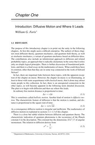
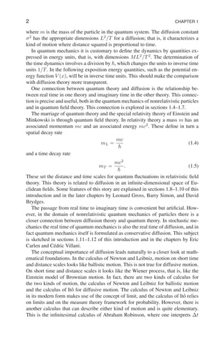
![INTRODUCTION 3
and ∆x as infinitesimal real numbers. It may be that this calculus is particularly
suitable for diffusive motion. This idea provides the theme in sections 1.13–1.14 of
this introduction and leads to the later contributions by Greg Lawler and Sam Buss.
The concluding section 1.15 connects earlier themes with a variation on musical
composition, presented in the final chapter by Julian Hook.
1.2 THE WIENER WALK
The Wiener walk is a mathematical object that is transitional between random walk
and the Wiener process. Here is the construction of the appropriate simple sym-
metric random walk. Let ξ1, . . . , ξn be a finite sequence of independent random
variables, each having the values ±1 with equal probability. One way to construct
such random variables is to take the set {−1, 1}n
of all sequences ξ of n values
±1 and give it the uniform probability measure. Then ξk is the kth element in the
sequence, and the function ξ 7→ ξk is the corresponding random variable. The ran-
dom walk is the sequence sk = ξ1 +· · ·+ξk defined for 0 ≤ k ≤ n. The underlying
probability space in this construction is finite, with 2n
points.
Here is the construction of the n-step Wiener walk on the time interval [0, T].
Let ∆t = T/n be the time step. Fix the diffusion constant σ2
> 0, and let the
corresponding space step be
∆x = σ
√
∆t. (1.6)
If
tk = k∆t (1.7)
for k = 0, 1, 2, . . . n, define
wn
(tk) = ξ1∆x + · · · + ξk∆x. (1.8)
Finally, define w(n)
(t) for real t with 0 ≤ t ≤ T by linear interpolation. Then
w(n)
is a random real continuous function defined on [0, T]. This random function
is the Wiener walk with time step ∆t = T/n. A typical sample path is illustrated
in Figure 1.1.
Let C([0, T]) be the metric space of all real continuous functions on the time
interval [0, T]. Let µ(n)
be the probability measure induced on Borel subsets of
C([0, T]) by the random function w(n)
. That is, the probability of a Borel subset
is the probability that the function w(n)
is in this subset. This probability measure
µ(n)
is the distribution of the Wiener walk. It is concentrated on a finite set of 2n
piecewise linear continuous paths.
1.3 THE WIENER PROCESS
The Wiener process is a fundamental object in probability theory, describing a par-
ticular kind of random path. Another common name for it is Brownian motion,
since it is closely related to the Einstein model for Brownian motion of a physical](https://image.slidesharecdn.com/17375049-250528112950-e20c26f6/85/Diffusion-Quantum-Theory-And-Radically-Elementary-Mathematics-Mn47-William-G-Faris-18-320.jpg)
![4 CHAPTER 1
10 20 30 40 50
t
-8
-6
-4
-2
2
x
Figure 1.1 A sample path of the Wiener walk.
particle. There are other models of the physical process of Brownian motion, so it
is clearer to use “Wiener process” for the mathematical object.
The Wiener process may be constructed in a number of ways, but one way to
get an intuition for it is to think of it as a limit of the Wiener walk. In this limit the
distribution of the Wiener walk, which is given by binomial probabilities, converges
to the distribution of the Wiener process, which is Gaussian.
PROPOSITION 1.1 (Construction of Wiener measure) For each n = 1, 2, 3, . . .
let µ(n)
be the probability measure defined on Borel subsets of C([0, T]) defined by
the Wiener walk with time step ∆t satisfying n∆t = T. Then there is a probability
measure µ defined on the Borel subsets of C([0, T]) such that µ(n)
→ µ as n → ∞
in the sense of weak convergence of probability measures.
This result may be found in texts on probability [2]. The statement about weak
convergence means that for each bounded continuous real function F defined on
the space C([0, T]) the expectation
R
F dµ(n)
→
R
F dµ as n → ∞. This µ is the
Wiener measure with diffusion parameter σ2
. If t is fixed, then the map w 7→ w(t)
is a function from the probability space C([0, T]) with Wiener measure µ to the real
numbers, and hence is a random variable. For each t ≥ 0 this random variable w(t)
has mean zero and variance σ2
t. Furthermore, the increments of w corresponding
to disjoint time intervals are independent. Since the random variable w(t) is the
sum of an arbitrarily large number of independent increments, by the central limit
theorem it must have a Gaussian distribution. The random continuous function w
associated with the Wiener measure is the Wiener process. A typical sample path
is sketched in Figure 1.2.
So far the Wiener process has been defined as a random continuous function
on a bounded interval [0, T] of time. However, it is not difficult to build the un-
bounded interval [0, +∞) out of a sequence of bounded intervals and thus give a](https://image.slidesharecdn.com/17375049-250528112950-e20c26f6/85/Diffusion-Quantum-Theory-And-Radically-Elementary-Mathematics-Mn47-William-G-Faris-19-320.jpg)
![INTRODUCTION 5
10 20 30 40 50
t
-0.6
-0.4
-0.2
0.2
0.4
x
Figure 1.2 A sample path of the Wiener process.
definition of the Wiener process as a random continuous function on this larger
time interval. In fact, it is even possible to define the Wiener process for the time
interval (−∞, +∞) as a random continuous function satisfying the normaliza-
tion w(0) = 0. Henceforth the Wiener process will refer to the probability space
C((−∞, +∞)) with the probability measure µ defined in this way.
In the following the expectation of a random variable F defined on the space
C((−∞, +∞)) with respect to the Wiener measure µ is written
µ[F] =
Z
F dµ. (1.9)
That is, the same notation is used for expectation as for probability. For example,
the expectation of w(t) (as a function of w) is µ[w(t)] = 0, and the variance is
µ[w(t)2
] = σ2
|t|.
Another useful topic is weighted increments of the Wiener process and the cor-
responding Wiener stochastic integral. Let t1 < t2, and consider the corresponding
increment w(t2) − w(t1). This is Gaussian with mean zero and variance σ2
(t2 −
t1) = σ2
|[t1, t2]|, which is proportional to the length of the interval. Consider two
such increments w(t2) − w(t1) and w(t′
2) − w(t′
1). The condition of independent
increments implies that they have covariance
µ[(w(t2) − w(t1))(w(t′
2) − w(t′
1))] = σ2
|[t1, t2] ∩ [t′
1, t′
2]|, (1.10)
which is proportional to the length of the intersection of the two intervals.
This generalizes to weighted increments. Let f be a real function such that
R ∞
−∞
f(t)2
dt < +∞. Then the Wiener stochastic integral
R ∞
−∞
f(t)d w(t) is a
well-defined Gaussian random variable with mean zero. Furthermore, the condi-
tion of independent increments implies that the covariance of two such stochastic
integrals is
µ
Z ∞
−∞
f(t) dw(t)
Z ∞
−∞
g(t′
) dw(t′
)
= σ2
Z ∞
−∞
f(t)g(t) dt. (1.11)](https://image.slidesharecdn.com/17375049-250528112950-e20c26f6/85/Diffusion-Quantum-Theory-And-Radically-Elementary-Mathematics-Mn47-William-G-Faris-20-320.jpg)
![6 CHAPTER 1
The independent increment property (1.10) is the special case when f and g are
indicator functions of intervals.
Another description of the Wiener process is by a partial differential equation.
For t 0 let ρ(y, t) (as a function of y) be the probability density of the Wiener
process at time t, so that
µ[f(w(t))] =
Z ∞
−∞
f(y)ρ(y, t) dy. (1.12)
Since the density ρ(y, t) is Gaussian with mean zero and variance σ2
t, it follows
that it satisfies the partial differential equation
∂ρ
∂t
=
1
2
σ2 ∂2
ρ
∂y2
. (1.13)
This is the simplest diffusion equation (or heat equation).
For a Wiener process describing diffusion in finite-dimensional Euclidean space
the probability density is jointly Gaussian. There is also a corresponding partial
differential equation, in which the second derivative in the space variable is replaced
by the Laplace operator.
Later it will appear that in infinite-dimensional space it is preferable to deal with
the Ornstein–Uhlenbeck velocity process instead of the Wiener process. The proba-
bility distributions are jointly Gaussian, but they have a more complicated time de-
pendence. They still solve a second-order linear partial differential equation. How-
ever, this equation involves the sum of the Laplace operator with another operator,
the first-order differential along the direction of a linear vector field.
1.4 DIFFUSION, KILLING, AND QUANTUM MECHANICS
The first remarkable discovery connecting quantum mechanics with diffusion the-
ory is that the fundamental equation of quantum mechanics is closely related to
an equation describing diffusion with killing. As we shall see, the connection is
through the Feynman–Kac formula.
Quantum theory, of course, is the ultimate mystery of modern science. It has
many strange features, such as remarkable correlations over long distances. These
correlations are experimentally observed, and their peculiar nature takes mathe-
matical shape in the form of a violation of Bell’s inequalities. The appendix to [17]
gives an account of this subject and its implications.
However strange quantum mechanics may be, there is universal agreement that
the wave function ψ for an isolated system satisfies the Schrödinger equation
∂ψ
∂t
= i
1
2
σ2 ∂2
∂x2
− V (x)
ψ. (1.14)
Here σ2
= ~/m and V (x) is the potential energy, here measured in inverse time
units.
This is often stated in terms of the Schrödinger operator H defined by
H = −
1
2
σ2 ∂2
∂x2
+ V (x). (1.15)](https://image.slidesharecdn.com/17375049-250528112950-e20c26f6/85/Diffusion-Quantum-Theory-And-Radically-Elementary-Mathematics-Mn47-William-G-Faris-21-320.jpg)
![INTRODUCTION 7
-3 -2 -1 1 2 3
x
-0.5
0.5
1
1.5
rate
Figure 1.3 A killing rate (potential) function with subtraction V (x) − λ0.
Then the Schrödinger equation (1.14) has the form
∂ψ
∂t
= −iHψ. (1.16)
This way of writing the equation differs slightly from the usual quantum mechan-
ical convention. The usual quantum mechanical potential energy and total energy
are obtained from the V and H in the present treatment by multiplication by the
constant ~. This converts inverse time units to energy units. In quantum mechanics
the dynamics is defined by dividing energy by ~, therefore returning to inverse time
units. So in the present notation, with inverse time units for H, the solution of the
Schrödinger equation with initial condition ψ(x) = ψ(x, 0) is
ψ(x, t) = (e−itH
ψ)(x). (1.17)
This operator exponential may be interpreted via spectral theory or by the theory
of one-parameter semigroups [9].
There are several connections between quantum mechanics and diffusion. The
most obvious ones are treated here in sections 1.4–1.7. There is also a more pro-
found connection between the Schrödinger equation and diffusion given by the
equations of stochastic mechanics. That will be the subject of sections 1.11–1.12.
A particularly simple way to go from quantum mechanics to diffusion is to re-
place it by t. The resulting diffusion equation is then
∂r
∂t
=
1
2
σ2 ∂2
∂x2
− V (x)
r. (1.18)
Here σ2
is interpreted as a diffusion constant. The diffusing particle randomly van-
ishes at a certain rate V (x) ≥ 0 depending on its position x in space. Thus there is
some chance that at a random time τ it will cease to diffuse and vanish. In proba-
bility it is common to say that the particle is killed. A typical killing rate function
V (x) is sketched in Figure 1.3. Actually, the sketch shows V (x) − λ0, where the
subtracted constant λ0 is the least eigenvalue of H.
The solution r(x, t) has a probability interpretation. Let r(y) be a given function
of the position variable y. Then r(x, t) is the expectation of r(y), when y is taken](https://image.slidesharecdn.com/17375049-250528112950-e20c26f6/85/Diffusion-Quantum-Theory-And-Radically-Elementary-Mathematics-Mn47-William-G-Faris-22-320.jpg)
![8 CHAPTER 1
as the random position of the diffusing particle at time t ≥ 0, provided that the
particle was started at x at time 0 and has not yet vanished. (The contribution to the
expected value for a particle that has vanished is zero.) The initial condition for the
equation is r(x, 0) = r(x). The equation
∂r
∂t
= −Hr (1.19)
has an operator solution, this time of the form
r(x, t) = (e−tH
r)(x). (1.20)
This operator exponential may also be interpreted via spectral theory or by the
theory of one-parameter semigroups. However, in this case there is also a direct
probabilistic solution of equation (1.18) given by the Feynman–Kac formula.
PROPOSITION 1.2 (Diffusion with killing: The Feynman–Kac formula) The so-
lution of the equation for diffusion with killing is given by
r(x, t) = µ
h
e−
R t
0
V (x+w(s)) ds
r(x + w(t))
i
. (1.21)
This says that the solution is obtained by letting the particle diffuse according to
a Wiener process, but with a chance to vanish from its current location in space at
a rate proportional to the value of V at this location. The exponential factor is the
probability that the particle has not yet vanished at time t. There are discussions of
the Feynman–Kac formula in Nelson’s article [6] on the Feynman integral and in
the book by Simon [16] on functional integration.
1.5 DIFFUSION, DRIFT, AND QUANTUM MECHANICS
Another connection of quantum mechanics with diffusion is more subtle. Instead
of diffusion with killing, there is diffusion with a drift that maintains equilibrium.
Let H be the Schrödinger operator (1.15) of section 1.4, expressed as before
in inverse time units. Suppose that H has an an eigenfunction ψ0(x) 0 with
eigenvalue λ0. Thus
−
1
2
σ2 ∂2
∂x2
+ V (x)
ψ0 = λ0ψ0. (1.22)
This gives a particular decay mode solution of the diffusion with killing equa-
tion (1.18) of the form r0(x, t) = e−λ0t
ψ0(x).
The interpretation in terms of diffusion with drift comes from the change of
variable r(x, t) = f(x, t)e−λ0t
ψ0(x). In other words, f(x, t) is the ratio of the
solution to the decay mode solution, which is seen to satisfy the partial differential
equation
∂f
∂t
=
1
2
σ2 ∂2
∂x2
+ u(x)
∂
∂x
f. (1.23)
Here the function u(x) represents a drift vector field given by
u(x) = σ2 1
ψ0(x)
∂ψ0(x)
∂x
. (1.24)](https://image.slidesharecdn.com/17375049-250528112950-e20c26f6/85/Diffusion-Quantum-Theory-And-Radically-Elementary-Mathematics-Mn47-William-G-Faris-23-320.jpg)
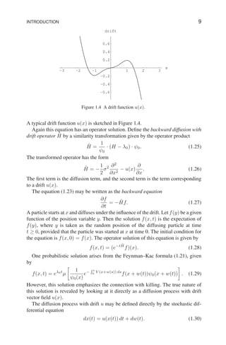
![10 CHAPTER 1
with the initial condition x(0) = x. The first term on the right represents the effect
of the systematic drift, while the second term on the right represents the influ-
ence of random diffusion. This equation involves the Wiener path, which is non-
differentiable with probability 1. However it may be formulated in integrated form
as
x(t) − x =
Z t
0
u(x(s)) ds + w(t). (1.31)
For each continuous path w(t) this equation determines a corresponding continuous
path x(t). Since the w(t) paths are random (given by the Wiener process), the x(t)
paths are also random. In particular, let f(y) be a function of the space variable,
and consider the expectation
f(x, t) = µ[f(x(t)) | x(0) = x] (1.32)
as a function of time and the starting position.
PROPOSITION 1.3 (Diffusion with drift: Stochastic differential equation) Sup-
pose the diffusion with drift process x(t) is defined by the stochastic differential
equation with the initial condition x(0) = x. Then the expectation f(x, t) satisfies
the backward diffusion with drift equation.
In other words, the expectation satisfies equation (1.23). This result is standard in
the theory of Markov diffusion processes. A charming account is found in Nelson’s
book [7].
1.6 STATIONARY DIFFUSION
Another way of describing diffusion with drift is in terms of probability density.
Say that instead of starting the diffusing particle at a fixed point, its starting point is
random with probability density ρ(x). Then, after time t, the probability will have
diffused to ρ(y, t). Thus, if one computes the expectation of a function f(y) of the
position at time t, one gets
Z ∞
−∞
f(y)ρ(y, t) dy =
Z ∞
−∞
f(x, t)ρ(x) dx. (1.33)
The density satisfies a partial differential equation, the forward equation (or
Fokker–Planck equation). It is
∂ρ
∂t
=
1
2
σ2 ∂2
∂y2
−
∂
∂y
u(y)
ρ. (1.34)
Again this has an operator form. Define the forward diffusion with drift operator
Ĥ′
by another similarity transformation, this time given by the operator product
Ĥ′
= ψ0 · (H − λ0) ·
1
ψ0
. (1.35)
This has the form
Ĥ′
= −
∂
∂y
1
2
σ2 ∂
∂y
− u(y)
. (1.36)](https://image.slidesharecdn.com/17375049-250528112950-e20c26f6/85/Diffusion-Quantum-Theory-And-Radically-Elementary-Mathematics-Mn47-William-G-Faris-25-320.jpg)
![INTRODUCTION 11
-3 -2 -1 1 2 3
x
0.1
0.2
0.3
0.4
0.5
density
Figure 1.5 A stationary density ρ0(x).
The equation
∂ρ
∂t
= −Ĥ′
ρ (1.37)
has an operator solution
ρ(y, t) = (e−tĤ′
ρ)(y). (1.38)
Let
ρ0(x) = ψ0(x)2
. (1.39)
Then ρ0 is interpreted as an equilibrium probability density. The drift u may be
expressed directly in terms of ρ0 by
u(x) =
1
2
σ2 1
ρ0(x)
∂ρ0(x)
∂x
. (1.40)
Say that the initial probability density ρ(x) = ρ0(x), the probability density that
defines the diffusion process. Then since Ĥ′
ρ0 = 0 the density remains the same;
that is, ρ(x, t) = ρ0(x) for all t. This is the stationary diffusion process. A typical
stationary density is shown in Figure 1.5.
Since the stationary diffusion process is defined from the process with killing
by a similarity transformation, the measure associated with the stationary diffusion
process may be defined in terms of the killing rate V (y) by
µ̂[F] = eT λ0
Z
ρ0(x)µ
F
1
ψ0(x)
e−
R T
0
V (x+w(s)) ds
ψ0(x + w(T))
dx. (1.41)
Here F depends on the path x(s) for s between time 0 and time T. Since ρ0(x) =
ψ0(x)2
this is equivalent to
µ̂[F] = eT λ0
Z
µ[Fψ0(x)e−
R T
0
V (x+w(s)) ds
ψ0(x + w(T))] dx. (1.42)
This suggests that it should be possible to construct the stationary diffusion with
drift measure directly from the Wiener measure with killing, without using the](https://image.slidesharecdn.com/17375049-250528112950-e20c26f6/85/Diffusion-Quantum-Theory-And-Radically-Elementary-Mathematics-Mn47-William-G-Faris-26-320.jpg)
![12 CHAPTER 1
10 20 30 40 50
t
-2
-1
1
2
x
Figure 1.6 A sample path of a nonlinear diffusion dx = u(x) dt + dw(t).
knowledge of the ground state wave function ψ0(x). This sort of construction turns
out to be useful in the field theory context discussed in sections 1.8–1.10. Let
µ̂T [F] =
1
ZT
µ[Fe−
R T
0
V (w(s)) ds
δ(w(T))]. (1.43)
This is the Wiener expectation, conditioned on returning to 0 after time T and on
not vanishing. The delta function enforces the condition of return to the origin,
and the ZT in the denominator is the probability of not vanishing along the way.
Suppose that T is large and that F depends only on part of the path well in the
interior of the interval from 0 to T. The expectations should then look much like
the expectations for the stationary diffusion process.
This gives a peculiar but useful view of the stationary diffusion process in terms
of the killing process. The diffusing particle starts at zero and is lucky enough
both to survive and to return to zero. Along the way it appears to be diffusing
in equilibrium. However, this equilibrium is maintained at the cost of the many
unsuccessful attempts that are discarded. A sketch of a typical sample path is shown
in Figure 1.6.
The transition from quantum mechanics to diffusion is computationally difficult.
In fact, the first step is to start with the function V (x) and solve the eigenvalue
equation for the ground state wave function ψ0(x).
Going the other way is easier. Start with ψ0(x) or with ρ0(x) = ψ0(x)2
. Then
u(x) =
1
2
σ2 ∂ log(ρ0(x))
∂x
, (1.44)
and V (x) − λ0 is recovered from
V (x) − λ0 =
1
2σ2
u(x)2
+
1
2
∂u(x)
∂x
. (1.45)
This, in fact, is the way the illustrations in the preceding sections were conceived.](https://image.slidesharecdn.com/17375049-250528112950-e20c26f6/85/Diffusion-Quantum-Theory-And-Radically-Elementary-Mathematics-Mn47-William-G-Faris-27-320.jpg)
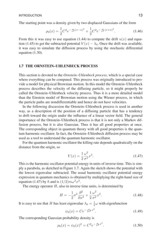
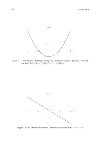
![INTRODUCTION 15
The drift in the diffusion process works out to be the linear drift
u(x) = −ωx. (1.51)
This linear drift is sketched in Figure 1.8. Nothing could be simpler.
The Ornstein–Uhlenbeck process x(t) may be defined by the linear stochastic
differential equation (the Langevin equation)
dx(t) = −ωx(t) dt + dw(t) (1.52)
with the initial condition x(0) = x. The first term on the right is a drift toward the
origin depending linearly on the distance, while the second term on the right is the
random diffusion term.
PROPOSITION 1.4 (Ornstein–Uhlenbeck process: Differential equation) The
Langevin stochastic differential equation for the Ornstein–Uhlenbeck process has
the explicit solution given for t ≥ 0 by
x(t) = e−ωt
x +
Z t
0
e−ω(t−s)
dw(s). (1.53)
This is a Wiener stochastic integral, so each x(t) is Gaussian. Furthermore, the
conditional mean is given by the exponential decay factor
x̄(t) = µ[x(t) | x(0) = x] = e−ωt
x. (1.54)
By (1.11) the conditional covariance is
µ[(x(t) − x̄(t))(x(t′
) − x̄(t′
)) | x(0) = x] = σ2
Z t∧t′
0
e−ω(t−s)
e−ω(t′
−s)
ds.
(1.55)
Here t ∧ t′
denotes the minimum of t and t′
. This integral is elementary; the result
is that the conditional covariance of x(t) is given by
µ[(x(t) − x̄(t))(x(t′
) − x̄(t′
)) | x(0) = x] =
σ2
2ω
(e−ω|t−t′
|
− e−ω(t+t′
)
). (1.56)
In particular, x(t) has conditional variance
µ[(x(t) − x̄(t))2
| x(0) = x] =
σ2
2ω
(1 − e−2ωt)
). (1.57)
If the time t 0 is large, then the Ornstein–Uhlenbeck process is in a sta-
tionary equilibrium state. In this case x(t) has mean zero and variance σ2
/(2ω).
Furthermore, it is Gaussian, as shown in Figure 1.9. The covariance is obtained by
multiplying the variance by the exponential decay factor e−ω|t−t′
|
.
For t 0 let gt be the Gaussian density with mean zero and variance given
by (σ2
/ω)(1 − e−2ωt
). The famous Mehler formula, expressed in terms of such a
Gaussian density, follows immediately from the calculation of the conditional mean
and variance and the fact that x(t) is Gaussian.
PROPOSITION 1.5 (Ornstein–Uhlenbeck process: Mehler formula) Let x(t) dif-
fuse according to the Ornstein–Uhlenbeck process. For every bounded measurable
function f the conditional expectation for t 0 is given by the integral
f(x, t) = µ[f(x(t)) | x(0) = x] =
Z ∞
−∞
gt(y − e−ωt
x)f(y) dy. (1.58)](https://image.slidesharecdn.com/17375049-250528112950-e20c26f6/85/Diffusion-Quantum-Theory-And-Radically-Elementary-Mathematics-Mn47-William-G-Faris-30-320.jpg)

![INTRODUCTION 17
10 20 30 40 50
t
-2
-1
1
2
x
Figure 1.10 A sample path of the Ornstein–Uhlenbeck process dx = −ωx dt + dw(t).
of a molecule in a fluid as a function of time, you get a picture somewhat like this.
It is a relatively featureless object. On the other hand, a detailed understanding of
the Ornstein–Uhlenbeck process (and its higher dimensional generalization) is the
starting point for progress in field theory.
1.8 EUCLIDEAN FIELD THEORY
The contributions in this volume by Simon and by Brydges touch on issues of quan-
tum field theory and stochastic field theory. This section gives background material
for reading their contributions. The main subject is the Euclidean free field, which is
the infinite-dimensional analog of the stationary Ornstein–Uhlenbeck diffusion pro-
cess. This is a first step toward constructing more general Euclidean fields, which
would be an infinite-dimensional analog of more general stationary diffusion pro-
cesses. This is again to be accomplished by conditioning, but there are new prob-
lems owing to large fluctuations. Simon’s book [15] gives a more complete account
of these matters; the work of Glimm and Jaffe [3] is an authoritative treatment.
Fundamental relativistic physical theory is currently formulated in terms of quan-
tum fields. Particles emerge in a secondary way, and the number of particles is not
a conserved quantity. The physical interpretation of quantum field theory is beyond
the scope of this introduction, so this account will focus on the rather artificial case
of scalar fields.
A subject of intrinsic interest in physics is Minkowski quantum field theory. This
is the theory of quantum fields defined on Minkowski space-time M with n − 1
space dimensions and one time dimension. It is a difficult subject both technically
and conceptually. However, there is a close connection between it and Euclidean
stochastic field theory. The latter is the theory of random functions defined on n-](https://image.slidesharecdn.com/17375049-250528112950-e20c26f6/85/Diffusion-Quantum-Theory-And-Radically-Elementary-Mathematics-Mn47-William-G-Faris-32-320.jpg)
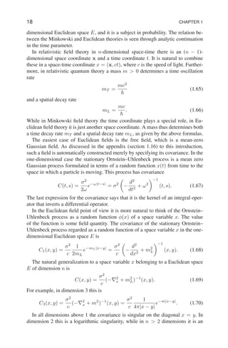
![INTRODUCTION 19
inverse n−2 power. This means that a random function with this covariance would
have to have an infinite variance. Finiteness is restored by having random variables
that are Schwartz distributions (generalized functions). That is, they are defined not
on points but on test functions. A test function is a function that is smooth and
sufficiently rapidly decreasing. The random variable is then
φ(f) =
Z
φ(x)f(x) dn
x, (1.71)
where the right-hand side is only a formal expression. The field φ(x) is only a
formal expression. It fails to exist as a function because it oscillates too much on
small distance scales, The averaged object φ(f) is defined because the oscillations
are cancelled by averaging with a smooth weight function.
The covariance of φ(f) with φ(g) is
C(f, g) =
Z Z
f(x)C(x, y)g(y) dn
x dn
y. (1.72)
This is well defined, since the integral on the right is finite. In particular, the vari-
ance of φ(f) is
C(f, f) =
Z Z
f(x)C(x, y)f(y) dn
x dn
y. (1.73)
All we need to know about the covariance is that this variance is finite. Then we
automatically have mean zero Gaussian random variables that are Schwartz distri-
butions.
Let µ be the probability measure defining the random Schwartz distributions
that constitute the Euclidean free field. The natural analogy with the Feynman–Kac
formula might lead us to define non-Gaussian measures by
µ̂[F] =
1
ZΛ
µ
F(φ) exp
−
Z
Λ
V (φ(x)) dn
x
. (1.74)
Here Λ is a large box, and the φ(x) is conditioned to be zero on the boundary of the
box. This is the analog in higher dimensions of the stationary process started at a
fixed time and conditioned to survive and return to the starting point at a later fixed
time. In that case the exponential factor describes the survival in the face of possible
killing in regions of space with large potential V , and the delta function enforces the
return. In the field theory case the exponential factor penalizes field configurations
with large values of the potential V , and the zero boundary condition pins the field
values on the sides of the box.
The problem is that it is a delicate matter to define nonlinear functions of
Schwartz distributions. A naive attempt would be to define V (φ)(f) to be V (φ(f)).
The calculation
Z
V (φ(x))f(x) dn
x 6= V
Z
φ(x)f(x) dn
x
(1.75)
shows that this is misguided. The right-hand side V (φ(f)) is defined. But it obvi-
ously does not give a good definition of the left-hand side. Therefore it is striking
that there are situations where it is possible to define a polynomial in the field,](https://image.slidesharecdn.com/17375049-250528112950-e20c26f6/85/Diffusion-Quantum-Theory-And-Radically-Elementary-Mathematics-Mn47-William-G-Faris-34-320.jpg)
![20 CHAPTER 1
in fact, a Wick power. As explained in the appendix (section 1.16), the kth Wick
power : φ(x)k
: of a Gaussian field φ(x) looks formally like a polynomial of de-
gree k in φ(x). It may exist even when the ordinary power φ(x)k
does not exist.
The reason is that the expectation of the product of the Wick power : φ(x)k
: with
the Wick power : φ(y)k
: is k!C(x, y)k
. The covariances C(x, x) and C(y, y) do
not enter into the expectation.
PROPOSITION 1.6 (Wick powers of the Gaussian free field) Suppose that for
some integer power k ≥ 1 the integral
Z Z
g(x)C(x, y)k
g(y) dn
x dn
y ∞ (1.76)
for each test function g. Then the kth Wick power : φk
(x) : exists as a random
distribution.
Here is a quick calculation to show that the integral condition (1.76) is just what
is needed. To say that the formal expression : φ(x)k
: exists as a random distribution
is to say that for each test function g the integral
: φk
: (g) =
Z
: φk
(x) : g(x) dn
x (1.77)
is a well-defined random variable. Compute the variance of such a Wick power by
µ[(: φk
: (g))2
] =
Z Z
g(x)µ[: φk
(x) : : φk
(y) :]g(y) dn
x dn
y
=
Z Z
g(x)C(x, y)k
g(y) dn
x dn
y. (1.78)
The integral condition (1.76) on the kth power of the covariance implies that the
corresponding kth Wick power (1.77) random variable exists and has finite vari-
ance.
The Wick powers of Euclidean free fields exist when the dimension n of the
Euclidean space is 2. In that case C(x, y) has only a logarithmic singularity at x =
y, and so the the integrals are finite. This insight led eventually to the construction
of interacting non-Gaussian random fields on two-dimensional Euclidean space.
For more than two dimensions the singularities are considerably worse, and more
intricate renormalizations are required.
1.9 QUANTUM FIELD THEORY
The transition from Euclidean stochastic field theory to Minkowski quantum field
theory is also discussed in the contributions by Brydges and by Simon. Here we
supply some background and introduce logarithmic Sobolev inequalities, a subject
which is explored in much greater detail in the contribution by Gross.
The transition from a stationary (translation invariant) field to a dynamical de-
scription in terms of operators is by a process of conditioning on initial conditions](https://image.slidesharecdn.com/17375049-250528112950-e20c26f6/85/Diffusion-Quantum-Theory-And-Radically-Elementary-Mathematics-Mn47-William-G-Faris-35-320.jpg)
![INTRODUCTION 21
at time zero. The formulas for the free Euclidean field are explicit. The logarith-
mic Sobolev inequality is a first step toward controlling the dynamical operator for
interacting fields, at least for the case of fields defined on the plane.
The covariance (1.69) for the Euclidean free field has a singularity on the diago-
nal that is logarithmic when n = 2 and that is an inverse n − 2 power when n 2.
Think of x = (x, ct) as having a space part and an imaginary time part. Then this
singularity is integrable when one only integrates over (n − 1)-dimensional space.
For each test function f0 on (n − 1)-dimensional space, define the sharp-time field
as the integral
φt(f0) =
Z
φ(x, t)f0(x) dn−1
x. (1.79)
This field is a well-defined Gaussian random variable with finite covariance
µ[φs(f0)φt(g0)] =
Z Z
f0(x)C(x, s; y, t)g0(y) dn−1
x dn−1
y. (1.80)
The sharp-time fields φt(f0) for fixed values of t belong to a certain Hilbert space
of Schwartz distributions; this is a space in which diffusion can take place.
Again consider Euclidean space-time with coordinates x = (x, ct) and condition
on the fields φ(x, 0) at time zero. Write
C = σ2
−
∂2
∂t2
+ ω2
−1
, (1.81)
where ω is the positive square root of the partial differential operator
ω2
= −c2
∇2
x + m2
T . (1.82)
Then, in analogy with equation (1.67), the time dependence of the covariance is
C(s, t) =
1
2
σ2
ω−1
e−ω|t−s|
, (1.83)
so the covariance of the time zero fields is C00 = (1/2)σ2
ω−1
, which is invertible
with inverse C−1
00 = (2/σ2
)ω. According to the general results in the appendix
(section 1.16), the conditional mean operator is Kt = C0tC−1
00 . This is Kt =
e−ω|t|
. The conditional mean of the time t field given the time zero field φ0 is
µ∗
[φt(f0)] = hf0, Ktφ0i. In short,
µ∗
(φt) = Ktφ0 = e−ω|t|
φ0, (1.84)
where φ0 is the given time zero field. Again, from the general results the conditional
covariance is the covariance minus the covariance of the conditional means. This
gives
C∗
(s, t) =
1
2
σ2
ω−1
(e−ω|t−s|
− e−ω(|t|+|s|)
). (1.85)
In particular, the equal-time conditional covariance is
C∗
(t, t) =
1
2
σ2
ω−1
(1 − e−2ω|t|
). (1.86)
Choose a sufficiently small Hilbert space H+
0 of moderately smooth test func-
tions on (n − 1)-dimensional Euclidean space with a sufficiently large dual Hilbert](https://image.slidesharecdn.com/17375049-250528112950-e20c26f6/85/Diffusion-Quantum-Theory-And-Radically-Elementary-Mathematics-Mn47-William-G-Faris-36-320.jpg)
![22 CHAPTER 1
space H−
0 of moderately rough distributions. These are chosen so that C∗
(t, t) is of
trace class from H+
0 to H−
0 . For test functions f0 in H+
0 the corresponding fixed-
time fields φt(f0) live in H−
0 . Define a diffusive dynamics on the fixed-time fields
by taking conditional expectations given the time zero fields. Then for the time t
fields the conditional mean is e−ωt
φ0 and the conditional covariance is the C∗
(t, t)
given above.
PROPOSITION 1.7 (Gaussian free field: Mehler formula) Let γt be the Gaussian
measure with mean zero and covariance C∗
(t, t). Consider a bounded continuous
real function F on the Hilbert space H−
0 of fixed-time fields. Then the conditional
expectation of F evaluated on the field at time t 0 given the field at time zero is
implemented by an infinite-dimensional Mehler formula
(e−tĤ
F)(φ0) =
Z
F(e−ωt
φ0 + χ) dγt(χ). (1.87)
The theory of the infinite-dimensional Ornstein–Uhlenbeck semigroup with its
Mehler formula is available from several sources; one brief account is [1]. The field
χ(t) diffuses in the field space H−
0 with diffusion constant σ2
and drift given by
the −ω from equation (1.82) acting on the field. Since ω ≥ mT 0 the action
of exp(−tω) on H−
0 is stabilizing and produces a stationary process, the Euclidean
free field. The Mehler formula yields the expectation of this process at time t, given
the time-zero field.
Suppose a construction produces a random field on Euclidean space E of dimen-
sion n. One can think of the Euclidean space as having coordinates x = (x, ct),
where x is an ordinary space coordinate and t is imaginary time. Do we then have
a quantum field on Minkowski space M of dimension n? The strategy would be
to replace t by it and leave the space variables x alone. It turns out that there is
such an analytic continuation, but it is a subtle matter. The case of the free field is
relatively simple. The replacement leads from the Ornstein–Uhlenbeck semigroup
exp(−tĤ) in the case of the free Euclidean field to the harmonic oscillator evolu-
tion exp(−itĤ) in the case of the free Minkowski quantum field. For non-Gaussian
interacting fields the passage from Euclidean probability to Minkowski field theory
requires more work. At the outset one needs estimates on the interaction for the
Euclidean fields.
The logarithmic Sobolev inequality (or equivalently, the hypercontractivity con-
dition) gives such an estimate. The classic logarithmic Sobolev inequality is for
the generator Ĥ of the Ornstein–Uhlenbeck process or, equivalently, the quantum
mechanical harmonic oscillator. As explained in the contribution by Gross, a log-
arithmic Sobolev inequality is equivalent to a lower bound for certain Schrödinger
operators. The following lower bound is a consequence of this equivalence and of
the existence of a logarithmic Sobolev inequality for Gauss measure.
PROPOSITION 1.8 (Semiboundedness of Hamiltonians) Consider a real Hilbert
space H+
0 and a covariance operator ω−1
: H+
0 → H−
0 from it to its dual space.
Suppose that the time decay operators e−tω
for t ≥ 0 act in H−
0 as a strongly
continuous semigroup of operators. Let σ2
0 be a diffusion constant, and let γt](https://image.slidesharecdn.com/17375049-250528112950-e20c26f6/85/Diffusion-Quantum-Theory-And-Radically-Elementary-Mathematics-Mn47-William-G-Faris-37-320.jpg)
![INTRODUCTION 23
be the Gaussian measure with mean zero and covariance (σ2
/2)(1 − e−2ωt
)ω−1
.
Suppose that the covariance ω−1
is trace class, so that γt is supported on H−
0 .
Define the Ornstein–Uhlenbeck generator Ĥ by the Mehler formula
(e−tĤ
F)(φ) =
Z
F(e−ωt
φ + χ) dγt(χ). (1.88)
This acts in the space L2
of functions on H−
0 that are square integrable with re-
spect to γ∞. Suppose that there is a constant mT with ω ≥ mT 0. Consider a
real function V on H−
0 such that e
− V
mT is in L2
. Then the sum of the Ornstein–
Uhlenbeck generator with V is bounded below. That is,
Ĥ + V ≥ −mT log(ke
− V
mT k2) (1.89)
as quadratic forms.
The function V may be unbounded below, but the operator Ĥ + V is bounded
below. At first this result looks incredibly weak, since it holds only if the negative
singularity of V is extremely mild. The remarkable fact is that it is independent
of dimension. It even holds in infinitely many dimensions, and this makes possible
the application to quantum field theory. The contribution to this volume by Simon
explains Nelson’s application of this result to Wick powers [5] as a step in the con-
struction of random fields on two-dimensional Euclidean space. The contribution
by Brydges goes on to show how another idea of Nelson led to the construction
of the quantum field from the Euclidean field. An exposition by Nelson himself is
found in [10].
1.10 INTERSECTING PATHS AND LOCAL TIMES
The particle picture describes particles moving in space as a function of time. The
field picture describes fields defined on Euclidean space E (space and imaginary
time) or Minkowski space-time M (space and real time). There is a strong analogy,
but it is mainly through the mathematics. It is striking that there is another way
of describing fields in terms of a sea of particles (paths defined as functions of an
auxiliary parameter) moving in space E or space-time M. This auxiliary parame-
ter is a kind of artificial time; it should not be identified with ordinary time. The
ultimate result is a picture of fields represented in terms of diffusing particles in
space (functions of the artificial time). Each particle diffuses up to an exponentially
distributed random “time” τ (depending on the particle), at which point it vanishes.
Furthermore, each particle has a random ± “charge.” The field value φ(y) repre-
sents a “charge”-weighted sum involving the total amount of “time” each particle
in the sea spends at y.
There are several variants of this theory. The one described here is an early ver-
sion due to Wolpert. His first article [19] describes the theory of Wiener path in-
tersections and local times, and his second article [18] gives the particle picture
for Euclidean field theory. The idea behind these representations is that the central
limit theorem causes a weighted sum of the local times of many particles to be-
come a Gaussian field. In the contribution of Brydges there is some discussion of](https://image.slidesharecdn.com/17375049-250528112950-e20c26f6/85/Diffusion-Quantum-Theory-And-Radically-Elementary-Mathematics-Mn47-William-G-Faris-38-320.jpg)
![24 CHAPTER 1
a different mechanism whereby the sum of local times is related to the square of a
Gaussian field.
Consider a Wiener process in Euclidean space starting at a point x; for conve-
nience take the diffusion constant to be σ2
= 2. This process describes random
continuous paths t 7→ w(t) with values in E = Rn
, defined for t ≥ 0 and with
w(0) = x. It is interpreted as describing the path of a particle diffusing in space (or
Euclidean space-time) as a function of the auxiliary time parameter. The transition
density of w(t) is Gaussian; that is,
gt(y − x) = µx[δ(w(t) − y)] (1.90)
as a function of y is a Gaussian density with mean x and with covariance 2tIn,
where In denotes the identity matrix. The connection with field theory is that the
covariance of the free Euclidean field (1.69) on E = Rn
is proportional to
G(y − x) =
Z ∞
0
e−m2
t
gt(y − x) dt. (1.91)
The role of the exponential factor e−m2
t
is to represent the probability that the
particle has not yet vanished at “time” t.
Define the local time by
T(w, y) =
Z τ
0
δ(w(t) − y) dt. (1.92)
This measures the “time” spent at y by a particle that diffuses from x and vanishes
at random “time” τ. The rate of vanishing is the constant rate m2
0. This is a
formal expression, but it can be interpreted in the sense of distributions. Multiply by
a weight function that depends on y and then integrate over y; the result is a well-
defined random variable. For instance, if the weight function were the indicator
function of a region in space, this would represent the “time” that the particle spent
in this region until its death at “time” τ. The relation between the covariance and
the local time is
G(y − x) = µx[T(w, y)]. (1.93)
This is the covariance of the free Euclidean field. The expectation of a quantity
quadratic in the field is expressed in terms of an expectation linear in the local
time.
Consider a large box of volume V . Let N be a Poisson random variable with
mean α. Consider a random number N of independent Wiener processes wi(t)
starting at random points xi chosen independently and uniformly in the box. This
is the sea of diffusing particles. Each particle has a positive or negative random sign
σi = ±1, for i = 1, . . . , N, also chosen independently and with equal probability
for the two signs. (This might be thought of as a kind of charge.) Furthermore, each
of the particles diffuses according to a Wiener process with killing at the rate m2
.
The “time” the ith particle vanishes is τi.
Define a parameter λ by
1
λ
=
2
m2
α
V
. (1.94)](https://image.slidesharecdn.com/17375049-250528112950-e20c26f6/85/Diffusion-Quantum-Theory-And-Radically-Elementary-Mathematics-Mn47-William-G-Faris-39-320.jpg)
![INTRODUCTION 25
The α/V factor describes the average density of the starting points for the particles,
while the 1/m2
time factor represents how long the particle lives on the average.
For each particle there is a local time
T(wi, y) =
Z τi
0
δ(wi(t) − y) dt. (1.95)
Define the field
φλ(y) = λ
1
2
N
X
i=1
σiT(wi, y). (1.96)
For large expected number α of particles this is a small constant times a sum with
many terms, each of which is a sum of the local times of the particles at y, weighted
by the corresponding signs. As usual in the theory of Schwartz distributions this
makes sense if we cancel fluctuations by averaging:
φλ(f) =
Z
φλ(y)f(y) dy (1.97)
is a well-defined random variable.
PROPOSITION 1.9 (Local time and the free field (Wolpert)) The joint probability
distribution of the random variables φλ(f) defined in terms of the local times with
random signs converges as λ → 0 to the joint probability distribution of the random
Euclidean free fields φ(f).
His proof proceeds by computing moments. The computation of the covariance
helps explain the choice of the coefficient λ
1
2 . Since the random signs produce
considerable cancellation, the computation soon leads to the expression
µ[φλ(x)φλ(y)] = λαµ[T(w1, x)T(w1, y)]. (1.98)
The contribution to the expectation of the product of local times is twice the con-
tribution from the situation where x is visited before y. The particle starts off uni-
formly at x1 and diffuses until it reaches x and then continues to diffuse until it
reaches y and then eventually vanishes. The contribution from the diffusion from
x1 to x is 1/V times 1/m2
, since it has to get from the random x1 to x before it
vanishes. The contribution from the diffusion from x to y is G(y − x). So the final
result for the covariance is
µ[φλ(x)φλ(y)] = λα
2
V m2
G(y − x) = G(y − x). (1.99)
Wolpert proved that for diffusion in two-dimensional space one can define prod-
ucts of local times. In other words, for k independent diffusions in two dimensions
it is meaningful to consider
T(w1, y) · · · T(wk, y) =
Z τ1
0
· · ·
Z τk
0
δ(w1(t1) − y) · · · δ(wk(t) − y) dt1 · · · dtk.
(1.100)
Again this is interpreted by multiplying by a weight function depending on y and
integrating over y. The result is a well-defined random variable. It measures the](https://image.slidesharecdn.com/17375049-250528112950-e20c26f6/85/Diffusion-Quantum-Theory-And-Radically-Elementary-Mathematics-Mn47-William-G-Faris-40-320.jpg)
![26 CHAPTER 1
amount of “time” that each of the k independently diffusing particles are simulta-
neously at the same point in the plane.
Wolpert’s construction of φλ(y) as a weighted sum of local times does not lead
to a definition of the power φλ(y)k
. The trouble is this power measures the amount
of “time” wi1
(t) = wi2
(t) = · · · = wik
(t) for each sequence i1, . . . , ik. However,
this will be infinite when two of the indices coincide.
The Wick power is obtained by writing the power of the sum as a sum of products
according to the usual distributive law, but retaining only the products involving
distinct paths. Thus it is
: φλ(y)k
: = λ
k
2
X
i1,...,ik
σi1
· · · σik
T(wi1
, y) · · · T(wik
, y), (1.101)
where the indices are required to be distinct.
PROPOSITION 1.10 (Local time and Wick powers (Wolpert)) Consider the spe-
cial case of two-dimensional Euclidean space. The joint distribution of the Wick
powers : φk
λ : (g) defined in terms of the local times with random signs converges
as λ → 0 to the Euclidean free field joint distribution of the usual Wick powers
: φk
: (g).
This result shows that intersections of diffusion paths are relevant to field theory.
The definition of the time that several diffusing particles are at the same point leads
to an alternate definition of nonlinear functions of random fields.
1.11 STOCHASTIC MECHANICS
It is already a remarkable fact that there is a diffusion process associated with the
ground state of a quantum mechanical system. However, there is a diffusion pro-
cess associated with an arbitrary solution of the Schrödinger equation (1.102). This
picture of quantum mechanics is stochastic mechanics. The contribution of Eric
Carlen in this volume gives an introduction to this subject. Nelson’s book [7] is the
classic source.
Throughout the following discussion the function V (x) has inverse time units.
Thus it is the usual potential energy function divided by Planck’s constant ~. As
usual σ2
= ~/m is the diffusion constant associated with mass m. Suppose that ψ
satisfies the time-dependent Schrödinger equation
∂ψ
∂t
= i
1
2
σ2 ∂2
ψ
∂x2
− V (x)ψ
. (1.102)
Let
ψ = ReiS
, (1.103)
and define the position density
ρ = R2
, (1.104)](https://image.slidesharecdn.com/17375049-250528112950-e20c26f6/85/Diffusion-Quantum-Theory-And-Radically-Elementary-Mathematics-Mn47-William-G-Faris-41-320.jpg)
![INTRODUCTION 27
the osmotic velocity
u = σ2 1
R
∂R
∂x
, (1.105)
and the current velocity
v = σ2 ∂S
∂x
. (1.106)
PROPOSITION 1.11 (Stochastic mechanics: Stochastic differential equation)
Suppose a solution of the time-dependent Schrödinger equation has osmotic and
current velocity fields u and v. Consider the diffusion process defined by the quan-
tum mechanical position density ρ at the initial time and by the stochastic differen-
tial equation
dx(t) = [u(x(t), t) + v(x(t), t)] dt + dw(t). (1.107)
Then this process has the correct quantum mechanical position density ρ at all
times.
Equation (1.107) defines the diffusion process for stochastic mechanics. This
should be distinguished from Bohmian mechanics, which is obtained by dropping
the osmotic velocity and the diffusion and solving only dx(t) = v(x(t), t) dt.
Since the vector fields u and v depend on space and time in a complicated way,
one must solve equations equivalent to the Schrödinger equation in order to define
the process. These equations are worth a closer inspection. The equation for u may
be written
uρ =
σ2
2
∂ρ
∂x
. (1.108)
This is the detailed balance condition, but only for the osmotic part of the velocity.
In the R and S variables the Schrödinger equation (1.102) takes the form
∂R
∂t
= −σ2
∂R
∂x
∂S
∂x
+ R
∂2
S
∂x2
(1.109)
and
∂S
∂t
=
1
2
σ2
1
R
∂2
R
∂x2
−
∂S
∂x
2
#
− V (x). (1.110)
Since ρ and u are defined in terms of R and v in terms of S this gives the following
result.
PROPOSITION 1.12 (Stochastic mechanics: Conservative diffusion) The
Schrödinger equation in the variables S and ρ takes the form
∂ρ
∂t
= −
∂vρ
∂x
(1.111)
and
∂S
∂t
=
1
2
∂u
∂x
+
1
2σ2
(u2
− v2
) − V (x). (1.112)](https://image.slidesharecdn.com/17375049-250528112950-e20c26f6/85/Diffusion-Quantum-Theory-And-Radically-Elementary-Mathematics-Mn47-William-G-Faris-42-320.jpg)
![28 CHAPTER 1
The first equation (1.111) is the equation of continuity. The second equa-
tion (1.112) is the dynamical equation that completes the determination of R and
S. From the equation (1.108) for u and the equation of continuity (1.111) for v we
get
∂ρ
∂t
=
1
2
σ2 ∂2
ρ
∂x2
−
∂((u + v)ρ)
∂x
. (1.113)
This is the forward equation for diffusion with diffusion constant σ2
and drift u+v.
It is curious how it comes from combining two separate equations.
1.12 VARIATIONAL PRINCIPLES AND MASS TRANSPORT
In mathematical physics there are two famous variational principles:
• Classical mechanics: The principle of stationary action.
• Quantum mechanics: The Rayleigh–Ritz principle for the ground state.
The Guerra–Morato variational principle includes both as special cases. This sec-
tion gives a brief introduction to this story. The contributions to this volume by
Carlen and Villani provide more information on the context of this and other varia-
tional principles. The book of Nelson [12] presents the connection with stochastic
mechanics. The present introductory account is partly suggested by Lafferty’s work
[4].
In section 1.11 the solution ψ of the time-dependent Schrödinger equa-
tion (1.102) was written in the form ψ = ReiS
. Furthermore, the osmotic veloc-
ity variable u was defined in equation (1.105) as σ2
times the spatial logarithmic
derivative of R, and the current velocity variable v was defined in equation (1.106)
as σ2
times the spatial derivative of S. The equations for R and S satisfy a varia-
tional principle. That is, there is an action functional such that these equations are
the Euler–Lagrange equations that express stationary action. This Guerra–Morato
action is
A =
Z T
0
Z ∞
−∞
1
2σ2
(v2
− u2
) − V (x)
ρ dx dt. (1.114)
The convention is the same as before; the function V (x) has inverse time units.
This action is a precise quantum mechanical analog of the usual action in classical
mechanics. In the form here it is dimensionless, but when it is multiplied by ~ it
has the dimensions of an action.
In Lafferty’s approach this action is regarded as a function of the probability den-
sity ρ = R2
. The variables u and v are determined in terms of ρ by the definitions
via equation (1.108) and by the equation of continuity (1.111). It is assumed that ρ
as a function of x is specified at the initial time t = 0 and the final time t = T.
The problem is to find a stationary point of a functional of a time-dependent
probability density ρ with its values specified at initial and final times. This is in
the spirit of the more general class of mass transport problems described by Villani.](https://image.slidesharecdn.com/17375049-250528112950-e20c26f6/85/Diffusion-Quantum-Theory-And-Radically-Elementary-Mathematics-Mn47-William-G-Faris-43-320.jpg)
![INTRODUCTION 29
PROPOSITION 1.13 (Stochastic mechanics: Action principle) Consider the
Guerra–Morato action as a function of a time-dependent probability density ρ with
its values specified at initial and final times. Then the stationary points of this action
satisfy the time-dependent Schrödinger equation.
The derivation is not difficult, but it is worth going through in order to understand
the role of the fixed initial and final conditions on the density. The differential δA
in terms of δρ, δu, and δv is
δA =
Z T
0
Z ∞
−∞
1
2σ2
(2vρ δv − 2uρ δu + v2
δρ − u2
δρ) − V (x)δρ
dx dt.
(1.115)
From the equation (1.108) we get
σ2
2
∂δρ
∂x
= ρ δu + u δρ. (1.116)
From the continuity equation (1.111) we get
∂δρ
∂t
= −
∂(ρ δv + v δρ)
∂x
. (1.117)
Insert these into the differential of the action. Then integrate by parts in the x vari-
able. This gives
δA =
Z T
0
Z ∞
−∞
S
∂δρ
∂t
+
1
2
∂u
∂x
+
1
2σ2
(u2
− v2
) − V (x)
δρ
dx dt.
(1.118)
If we fix ρ at times 0 and T, so that δρ = 0 at these times, then we may also
integrate by parts in the t variable and neglect the boundary terms. This gives the
final answer
δA =
Z T
0
Z ∞
−∞
−
∂S
∂t
+
1
2
∂u
∂x
+
1
2σ2
(u2
− v2
) − V (x)
δρ dx dt. (1.119)
The point at which δA vanishes is the solution of the Schrödinger equation.
1.13 PROBABILITY WITH INFINITESIMALS
The traditional framework for mathematical probability is an infinite sequence
ξ1, . . . , ξk, . . . of random variables, indexed by the natural numbers. Results are
stated in terms of a complicated limiting process. The nonstandard analysis of
Abraham Robinson gives an alternative model. For a brief account of its applica-
tion to probability, see the book by Nelson [13].
Nonstandard analysis is a theory in which each mathematical object is deter-
mined to be either standard or nonstandard. For instance, there is a theory of natural
numbers in which each natural number is either standard or nonstandard. The num-
ber 0 is standard, the number 1 is standard, the number 2 is standard, the number
3 is standard, and so on. If m is standard and n is nonstandard, then it follows that
m n. There are nonstandard natural numbers.](https://image.slidesharecdn.com/17375049-250528112950-e20c26f6/85/Diffusion-Quantum-Theory-And-Radically-Elementary-Mathematics-Mn47-William-G-Faris-44-320.jpg)
![INTRODUCTION 31
still consists of the copy of N and the copies of Z, but now N must be followed by
the copies of Z in some linear order.
These results already give a rather clear picture of what the nonstandard natu-
ral number system N∗
must be. It is a copy of N (the standard natural numbers)
followed by copies of Z lined up in some order.
There is an apparent conflict with mathematical practice: The induction princi-
ple seems to be violated. The induction principle states that every nonempty subset
has a least element. A perverse application to the subset of nonstandard elements
would give a contradiction. But induction is applied in ordinary mathematical prac-
tice only to subsets defined independently of the concepts “standard” and “nonstan-
dard.” Thus a cautious mathematician need not fear conflict.
It gets more interesting when one looks at arithmetic. The structure of addition
is reasonably clear. Suppose that N∗
is a set with two distinguished points 0 and 1
and with a function + from N∗
× N∗
to N∗
. Suppose that this defines an operation
that is associative and commutative and that has 0 as an additive identity element.
Define m ≤ n by the existence of k with m + k = n. Suppose that this defines a
linear order on N∗
. Suppose also that m ≤ 1 implies m = 0 or m = 1. Finally,
suppose that every number is even or odd. That is, suppose that for every n either
there exists k with k + k = n or there exists k with (k + k) + 1 = n. Then the
linearly ordered set N∗
consists of N followed by a number of copies of Z. These
copies of Z are themselves arranged in a dense linear order without least or greatest
element.
This makes the picture even more specific, especially if it is assumed that the set
N∗
is countable. Then the nonstandard natural number system N∗
is a copy of N
(the standard natural numbers) followed by copies of Z. The copies are themselves
lined up according to the same linear order as that of the rational numbers Q. See
[14] for more on the theory of addition.
The proof that a model of the theory of addition has its Z copies in a dense linear
order without least or greatest element follows from our knowing that each number
is either even or odd. Say that m n, that m is in one of the copies of Z, and that
n is in another copy of Z. By adding 1 if necessary we can arrange that m + n is
even. Then m+n = k +k, where k is also a natural number. We have m k n,
so it is clear that k cannot be standard. Furthermore, n − k = k − m. If k were in
the same copy of Z as m, then k − m would be standard, so n − k would also be
standard, and so also n = m + (k − m) + (n − k) would be in the same copy. This
is a contradiction. So k cannot be in the same copy of Z as m. In the same way, k
cannot be in the same copy as n. So there must be a copy of Z between the copy
associated with m and that associated with n. This proves that the copies are in a
dense linear order. In a similar way, one can prove that if n is nonstandard, then
n + n is in different copy of Z from that of n. This proves that there is no greatest
copy. Finally, one can prove that if n is nonstandard and even with n = k + k, then
k is nonstandard and is in a copy of Z that is different from that of n. This proves
that there is no least copy.
To summarize the external point of view, there is a system N of standard natu-
ral numbers and a larger system N∗
of natural numbers augmented by nonstandard
elements that are each larger than every standard natural number. The remarkable](https://image.slidesharecdn.com/17375049-250528112950-e20c26f6/85/Diffusion-Quantum-Theory-And-Radically-Elementary-Mathematics-Mn47-William-G-Faris-46-320.jpg)
![32 CHAPTER 1
thing is that the properties of these two natural number systems that may be stated in
elementary terms (i.e., in terms of 0, s, +, ·) are the same. In that sense, it is difficult
to distinguish between N and N∗
. The multiplicative structure of N∗
is extraordi-
narily complicated, since a lot of information about prime numbers is included. Of
course this is already true of N.
Return to the probability model of a sequence ξ1, . . . , ξn of random variables,
where n is nonstandard. Look more closely at the index set 1, . . . , n from the ex-
ternal point of view. It consists of all the standard natural numbers, followed by a
large number of copies of Z, concluding with a partial copy of Z ending in n. This
partial copy looks in its order structure like the natural numbers in reverse. Notice
that there is both a first element and a last element in this index set. Contrast this
with the conventional model for a large number of trials, which is an infinite se-
quence with a starting point but no end point. The nonstandard model might at first
appear to be more complicated. However, from the internal point of view, explained
below, it is no more complicated than any other finite sequence.
In the internal point of view [11] there is a natural number system N. (This would
be N∗
in the external point of view.) One recognizes that in this system there are
certain natural numbers that are standard and others that are nonstandard. This is a
discovery about the natural numbers rather than the creation of a new system. The
internal point of view leads to a particularly simple formulation of nonstandard
analysis. All that is needed is to augment set theory with one new predicate.
A common formalization of mathematics is Zermelo–Frankel set theory with
choice, or ZFC. The only primitive nonlogical symbol of ZFC is the ∈ symbol
that represents set membership. Everything else is defined in terms of this. Internal
Set Theory, or IST, consists of ZFC with a new predicate “standard.” The ZFC
set-building axioms are only used with expressions that do not involve this new
predicate. This is no restriction on conventional mathematics; every set that can be
defined in ZFC can also be defined in IST.
In IST there is a set N of natural numbers. A natural number n ∈ N is either
standard or nonstandard. There is no set of standard natural numbers. On the other
hand, there is a new kind of set formation that builds a standard set with specified
standard elements. Thus, for example, the standard set whose standard elements are
the standard natural numbers is N.
The syntactical formulation of nonstandard analysis has the advantage of sim-
plicity. One does not need to change the notions of natural numbers or real numbers.
The additional axioms only describe new aspects of them.
Return again to the probability model of the sequence ξ1, . . . , ξn of independent
±1 random variables, where n is nonstandard. From the internal point of view the
index set {1, . . . , n} is just a finite sequence of natural numbers, even though n is
nonstandard. And the fact that the variance of (ξ1 + · · · + ξn)/n is 1/n is the usual
calculation for a finite probability space. This variance 1/n is a fraction like any
other, though infinitesimal.
Axioms for set theory like ZFC thus do not give a clear intuition for mathemat-
ical systems, even those as seemingly elementary as the natural number system N.
Consider one mathematician who thinks that there are nonstandard elements of N
and another mathematician who has never considered this possibility. In all their in-](https://image.slidesharecdn.com/17375049-250528112950-e20c26f6/85/Diffusion-Quantum-Theory-And-Radically-Elementary-Mathematics-Mn47-William-G-Faris-47-320.jpg)
![34 CHAPTER 1
Let V be a vector space with a quadratic form having signature with a single +
(time) and the rest − (space). (This quadratic form is a pseudo-Riemannian metric;
see [8].) Let V act freely and transitively on a set M. Then M is Minkowski space,
consisting of events in space-time. If x 6= y are events, then y − x is timelike,
lightlike, or spacelike depending on whether the quadratic form is strictly positive,
zero, or strictly negative on this vector.
If y − x is timelike or lightlike, the time between x and y is the square root of
the value of the quadratic form and is denoted |y − x|. In the Minkowski case there
is an antitriangle inquality.
PROPOSITION 1.15 (Antitriangle inequality for Minkowski space) If x, y, z are
distinct events in M, if z − y and y − x are timelike, and if the unit vector (z −
y)/|z − y| minus the unit vector (y − x)/|y − x| is spacelike, then z − x is timelike
and
|z − x| |z − y| + |y − x|. (1.122)
The antitriangle inequality underlies the “twin brother paradox.” The event x is
the parting of two brothers. One brother continues in his state of uniform motion.
The other brother is more active; the event y is his change from one uniform motion
to another with the purpose of arranging a reunion. The event z is their reunion. The
passive brother has aged by |z − x|. The active brother has aged by |y − x| + |z −
y|, which is less. At the reunion the active brother not only looks younger, he is
younger. The disparity is no paradox; it is a consequence of the geometry of space-
time.
A possibly more sinister application of the antitriangle inequality is to
momentum-energy vectors. If u is a (timelike) momentum-energy vector of a
moving particle, then its length |u| = mc2
, which is the mass of the particle
given in energy units. Say that the particle splits into two moving particles, so
u = v+w, by conservation of momentum-energy. The antitriangle inequality gives
|u| |v| + |w|. In effect, mass is converted to relative motion. One hopes this has
benign consequences.
Replace Minkowski space M by Euclidean space E. Then quantum field theory
becomes Euclidean field theory, that is, a stochastic process in the framework of
ordinary probability theory. When all events are spacelike related, then the intricate
causal structure of the world is replaced by mere random fluctuation. This would
seem to wipe out most of what is interesting about quantum field theory. It is there-
fore remarkable that one can, in principle, recover the Minkowski quantum field
theory from the Euclidean stochastic field theory, as described in the contribution
to this volume by Brydges.
This mathematical framework for geometry may be generalized. Let G be an
abelian group. Let S be a set on which G acts freely and transitively. Thus if x is in
S and v is in G, then x + v is in S. Furthermore, given x, y in S, there is a unique
difference element y − x in G. Everything works the same in this more general
context, except that the combinations ax + by with a + b = 1 only make sense
when a, b are integers. Thus ax + by = x + b(y − x) is defined because y − x is
an element of an abelian group, and so it or its inverse may be repeatedly added to
itself to produce the integer multiple b(y − x).](https://image.slidesharecdn.com/17375049-250528112950-e20c26f6/85/Diffusion-Quantum-Theory-And-Radically-Elementary-Mathematics-Mn47-William-G-Faris-49-320.jpg)

![36 CHAPTER 1
new experimental number F(x).
For each subset A of S there is a corresponding indicator function 1A that is 1
on A and 0 on the complement of A. A subset A is said to be a measurable subset
if its indicator function is a measurable function. Many expositions of the concept
of measurable space take the notion of measurable subset as fundamental; this is
equivalent to the approach in the present exposition.
The third concept is that of expectation. Let F+ be the class of positive mea-
surable functions, that is, of measurable functions F such that F(x) ≥ 0 for all
x in S. The expectation µ : F+ → [0, ∞] is a function that is required to satisfy
certain linearity and continuity properties (monotone convergence). These are the
usual properties of the abstract Lebesgue integral; however, it is also required that
for each constant function c we have µ[c] = c. Let L1
be the class of all measurable
functions F such that µ[|F|] +∞. There is a natural definition of the expectation
as a linear function µ : L1
→ R. If F is in F+ or if F is in L1
, then the expectation
of F is well defined and is written µ[F]. When the set S, the class of measurable
functions F, and the expectation µ are given, then each measurable function F is
called a random variable. In general discussions an expectation is sometimes called
a probability measure; in concrete situations the expectation of a random variable
is often called its mean or sometimes average. A measurable space with a given
probability measure is called a probability space.
The word probability is often used in a narrower context. A measurable subset
A of a probability space is called an event. The probability of an event A is the
expectation of the indicator function of A and is written µ[A]. Many expositions of
probability begin with the probabilities of events as the fundamental concept; this is
equivalent to (actually a special case of) the present approach based on expectations
of random variables.
1.16.2 Conditional expectation
Let L2
⊂ L1
be the class of all real measurable functions with µ[F2
] ∞. This
is the class of random variables with finite variance. This class of functions forms
a natural real Hilbert space. The inner product of F and G is µ[FG].
The variance of F in L2
is
Var[F] = µ[(F − µ[F])2
]. (1.123)
If F and G are each in L2
, then they have a covariance. This is
Cov[F, G] = µ[(F − µ[F])(G − µ[G])]. (1.124)
The covariance is just the inner product of the components orthogonal to the con-
stant functions. The variance is a special case of covariance, since it is given by
Var[F] = Cov[F, F].
Consider a random variable F in L2
. Say that G1, . . . , Gk are random variables.
The conditional expectation of the random variable F given the random variables
G1, . . . , Gk is a random variable
µ[F | G1, . . . , Gk] = φ(G1, . . . , Gk). (1.125)](https://image.slidesharecdn.com/17375049-250528112950-e20c26f6/85/Diffusion-Quantum-Theory-And-Radically-Elementary-Mathematics-Mn47-William-G-Faris-51-320.jpg)
![INTRODUCTION 37
It is defined as the orthogonal projection of F onto the subspace of all L2
of the
form ψ(G1, . . . , Gk), where ψ is a Borel function. That is, φ is the Borel function
such that φ(G1, . . . , Gk) best approximates F in the L2
sense.
Sometimes it is nice to have a name for the Borel function φ from Rk
to R such
that the random variable φ(G1, . . . , Gk) from S to R best approximates F. The
usual notation is that the value of φ on t in Rk
is
φ(t1, . . . , tk) = µ[F | G1 = t1, . . . , Gk = tk]. (1.126)
This is the conditional expectation of F given that the random variables G1, . . . , Gk
have the particular values t1, . . . , tk.
Fix random variables G1, . . . , Gk. Consider the space G ⊂ F of all functions
ψ(G1, . . . , Gk), where ψ : Rk
→ R is a Borel function. Then G is a class of
functions that satisfies all the properties required to be a collection of measurable
functions. The functions in G compute those experimental numbers that can be
derived from knowing the experimental values of G1, . . . , Gk.
This leads to a more general concept of conditional expectation. Let G ⊂ F be
a class of measurable functions satisfying the properties of containing the constant
functions, being closed under composition with Borel functions, and being closed
under pointwise limits. Consider a random variable F in L2
. The conditional ex-
pectation of the random variable F given the class G of random variables is the
random variable µ[F | G] in L2
that is the orthogonal projection of F onto those
elements of L2
that are in G.
To compute with this definition, one needs only the concept of orthogonal pro-
jection. Consider F in L2
. To say that µ[F | G] is the orthogonal projection onto the
L2
functions in G is to say that µ[F | G] is in G, and that F −µ[F | G] is orthogonal
to G. This last condition says that for every L2
function G in G the identity
µ[FG] = µ[µ[F | G]G] (1.127)
is satisfied. Since this works in particular for G = 1, it follows that the expectation
µ[F] may be computed in stages: first the average based on the given extra informa-
tion µ[F | G] (which depends on the values of the functions in G), then the average
µ[µ[F | G]] over all possibilities for what that extra information might be. Typically
the two stages are the future prediction given the present, then all possibilities for
the present.
In many expositions of conditional expectation the role of the given class of
random variables G is played by a given class of events. The present definition is
equivalent to this, but gets directly to the point: the conditional expectation of a
random variable is a random variable, not an event.
The concept of conditional probability is a special case of the concept of condi-
tional expectation. The conditional probability P[A | G] of an event A given a class
G of measurable functions is the conditional expectation of the indicator function
of A given this class. Even in this case it is the concept of random variable that is
fundamental. The conditional probability of an event is not an event, or even the
indicator function of an event. It is a random variable.
The definition of conditional covariance is
Cov[F, G | G] = µ[(F − µ[F | G])(G − µ[G | G]) | G]. (1.128)](https://image.slidesharecdn.com/17375049-250528112950-e20c26f6/85/Diffusion-Quantum-Theory-And-Radically-Elementary-Mathematics-Mn47-William-G-Faris-52-320.jpg)
![38 CHAPTER 1
There is an identity
Cov[F, G] = µ[Cov[F, G | G]] + Cov[µ[F | G], µ[G | G]]. (1.129)
It says that the covariance is the expectation of the conditional covariance plus
the covariance of the conditional expectation. The obvious specialization says that
the variance is the expectation of the conditional variance plus the variance of the
conditional expectation.
1.16.3 Gaussian processes: Wick products
If F1, . . . , Fk are random variables, then they map the probability measure µ de-
fined as an expectation for functions on S to a probability measure µ∗ defined for
functions on Rk
. This measure µ∗ is called the distribution (or joint distribution) of
F1, . . . , Fk. It is defined for each Borel function φ ≥ 0 by
µ∗(φ) = µ[φ(F1, . . . , Fk)]. (1.130)
A stochastic process (or random process) is a family of random variables φ(x)
indexed by x in some set I. It is a Gaussian process if for each finite subset of I
the corresponding random variables have a joint Gaussian distribution.
A Gaussian process is defined by its mean function and its covariance function.
Consider an index set I. Consider a function M : I → R and a symmetric function
C : I × I → R with the positive definiteness property. (This means that on each fi-
nite subset of the index set it is ≥ 0 as a quadratic form.) Then there is a probability
measure µ and a family of random variables φ(x) indexed by x in I with mean
µ[φ(x)] = M(x) (1.131)
and covariance
µ[(φ(x) − M(x))(φ(y) − M(y))] = C(x, y) (1.132)
and such that the process is Gaussian.
Consider a mean-zero Gaussian process with covariance given by µ[φ(x)φ(y)] =
C(x, y). A nice feature is that it is easy to compute higher moments. The mth
moment µ[φ(x1) · · · φ(xm)] is the sum over all partitions P of {1, . . . , m} into two-
element subsets {i, j} of the product of the covariances C(xi, xj) corresponding to
the elements of the partition. That is,
µ[φ(x1) · · · φ(xm)] =
X
P
Y
{i,j}∈P
C(xi, xj). (1.133)
For example, the fourth moment is
µ[φ(x)φ(y)φ(z)φ(w)] = C(x, y)C(z, w) + C(x, z)C(y, w) + C(x, w)C(y, z).
(1.134)
Let F be the smallest space of measurable functions including all measurable
functions given by the mean zero Gaussian process. Denote the associated space
L2
of functions in F with finite variance by Γ. Then Γ has a natural decomposition.
Let Γ≤k be the closed subspace of Γ spanned by linear combinations of jth degree
monomials φ(x1) · · · φ(xj) with j ≤ k. Let Γk be the orthogonal complement of](https://image.slidesharecdn.com/17375049-250528112950-e20c26f6/85/Diffusion-Quantum-Theory-And-Radically-Elementary-Mathematics-Mn47-William-G-Faris-53-320.jpg)
![INTRODUCTION 39
Γk−1 in Γ≤k. This is the kth Wiener chaos subspace. (In field theory it would be
called the k particle subspace.) Then every random variable in Γ may be uniquely
decomposed as a sum of its projections onto the Γk.
One interesting projection is the simple case of the orthogonal projection of the
monomial φ(x1) · · · φ(xk) onto Γk. The resulting polynomial is the Wick product
: φ(x1) · · · φ(xk) :. Trivial cases include : 1 := 1 and : φ(x) := φ(x). Also, the
quadratic case
: φ(x)φ(y) := φ(x)φ(y) − C(x, y) (1.135)
is very familiar. The cubic case
: φ(x)φ(y)φ(x) := φ(x)φ(y)φ(z) − C(y, z)φ(x) − C(z, x)φ(y) − C(x, y)φ(z)
(1.136)
is more interesting, and the pattern continues.
According to the general rule, the covariance of the monomial φ(x1) · · · φ(xk)
with the monomial φ(xk+1) · · · φ(xm) is the sum over all partitions of {1, . . . , m}
into two-element subsets of the product of the covariance. For Wick products the
formula is different. The covariance of the Wick product : φ(x1) · · · φ(xk) : with
the Wick product : φ(xk+1) · · · φ(xm) : is the sum over a certain restricted class of
partitions of {1, . . . , m} into two-element subsets of the product of the covariances
associated with these subsets. The restriction is that no two-element subset in the
partition can be a subset of {1, . . . , k} or of {k + 1, . . . , m}. For example,
µ[: φ(x)φ(y) : : φ(z)φ(w) :] = C(x, z)C(y, w) + C(x, w)C(y, z). (1.137)
The projection takes out the internal covariances.
A Wick power is a special case of a Wick product. Thus the orthogonal projection
of φ(x)k
onto Γk is the Wick power : φ(x)k
:. For example, the quadratic case is
: φ(x)2
:= φ(x)2
− C(x, x), (1.138)
and the cubic case is
: φ(x)3
:= φ(x)3
− 3C(x, x)2
φ(x). (1.139)
The Wick powers resemble the familiar Hermite polynomials constructed by the
classical Gram–Schmidt orthogonalization process. The reader may be assured that
this is no coincidence.
The covariance of the Wick power : φ(x)k
: with the Wick power : φ(y)k
: is
Cov[: φ(x)k
:, : φ(y) :k
] = k!C(x, y)k
. (1.140)
Neither C(x, x) nor C(y, y) occurs in this formula. The natural nonlinear functions
of Gaussian random fields are not ordinary powers, but instead Wick powers.
1.16.4 Gaussian processes: Conditional expectation and covariance
For some purposes it is useful to take the index set for a Gaussian process to be a
vector space. One way to accomplish this is to define φ(f) =
P
x f(x)φ(x). Then
the index objects f belong to a vector space of functions. In other situations the
Gaussian process φ(f) indexed by f in a vector space can be the natural object
from the outset.](https://image.slidesharecdn.com/17375049-250528112950-e20c26f6/85/Diffusion-Quantum-Theory-And-Radically-Elementary-Mathematics-Mn47-William-G-Faris-54-320.jpg)


![O, Jens, boy, Jens! Truth above all things. Magna est veritas et
prævalebit. The Reverend Peter Nielsen entered, clean, in a
cassock, and with a shovel hat on his head.
The children whom you have seen, said Peter Nielsen, are the
nephews and nieces of my worthy housekeeper, Maria Grubbe. She
is a charitable woman, and as her sister is very poor, and has a large
family, my Maren, I mean my housekeeper, takes charge of some of
the overflow.[15]
It is a great burden to you, said the Canon.
Peter Nielsen shrugged his shoulders. To clothe the naked and give
food to the hungry are deeds of mercy.
I quite understand, quite, said the Canon.
I only mentioned it, continued the parish priest, lest you should
suppose—
I quite understand, said the Canon, interrupting him, with a bow
and a benignant smile.
And now, said Peter Nielsen, I am at your service.
Thereupon the Canon unfolded to his astonished hearer the nature
of his mission. The pastor sat listening attentively with his head
bowed, and his hands planted on his knees. Then, when his visitor
had done speaking, he thrust his left hand into his trouser pocket
and produced a palmful of carraway seed. He put some into his
mouth, and began to chew it; whereupon the whole room became
scented with carraway.
I am fond of this seed, said the priest composedly, whilst he
turned over the grains in his hand with the five fingers of his right.
It is good for the stomach, and it clears the brain. So I understand
that there are three parties?](https://image.slidesharecdn.com/17375049-250528112950-e20c26f6/85/Diffusion-Quantum-Theory-And-Radically-Elementary-Mathematics-Mn47-William-G-Faris-57-320.jpg)
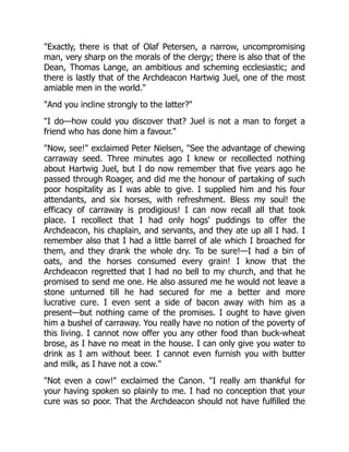

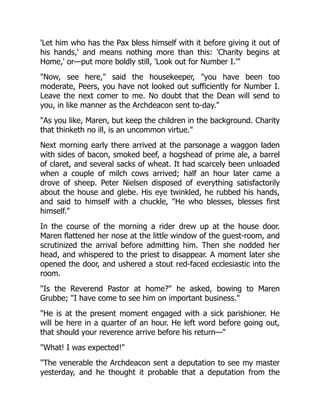
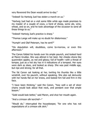


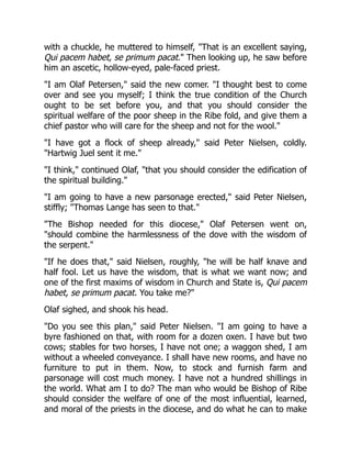
![Then he sat down.
For a moment there was silence, and then a storm broke loose.
Peter sat motionless, with his eyes fixed on the ground, motionless
as a rock round which the waves toss and tear themselves to foam.
Thus it came about that the twenty-ninth bishop of Ribe was Peter
Nielsen.
FOOTNOTE:
[15] In Norway, Denmark, Sweden, and Iceland, clerical celibacy was
never enforced before the Reformation. Now and then a formal
prohibition was issued by the bishops, but it was generally ignored.
The clergy were married, openly and undisguisedly.](https://image.slidesharecdn.com/17375049-250528112950-e20c26f6/85/Diffusion-Quantum-Theory-And-Radically-Elementary-Mathematics-Mn47-William-G-Faris-68-320.jpg)
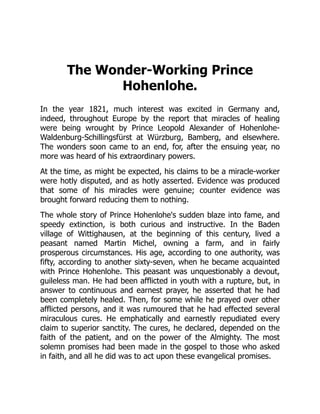
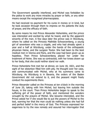
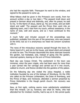
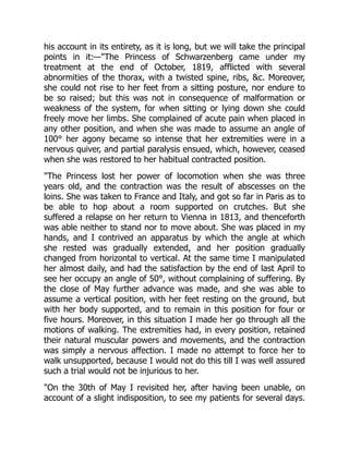
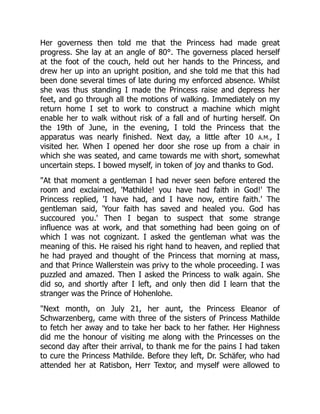
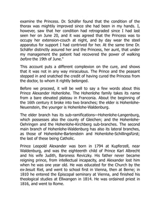
![Dr. Wolff, the father of Sir Henry Drummond Wolff, in his Travels
and Adventures, which is really his autobiography, says (vol i. p.
31):—
Wolff left the house of Count Stolberg on the 3rd April, 1815, and
went to Ellwangen, and there met again an old pupil from Vienna,
Prince Alexander Hohenlohe-Schillingsfürst, afterwards so celebrated
for his miracles—to which so many men of the highest rank and
intelligence have borne witness that Wolff dares not give a decided
opinion about them. But Niebuhr relates that the Pope said to him
himself, speaking about Hohenlohe in a sneering manner, 'Questo far
dei miracoli!' This fellow performing miracles!
It may be best to offer some slight sketch of Hohenlohe's life. His
person was beautiful. He was placed under the direction of Vock, the
Roman Catholic parish priest at Berne. One Sunday he was invited to
dinner with Vock, his tutor, at the Spanish ambassador's. The next
day there was a great noise in the Spanish embassy, because the
mass-robe, with the silver chalice and all its appurtenances, had
been stolen. It was advertised in the paper, but nothing could be
discovered, until Vock took Prince Hohenlohe aside, and said to him,
'Prince, confess to me; have you not stolen the mass-robe?' He at
once confessed it, and said that he made use of it every morning in
practising the celebration of the mass in his room; which was true.
(This was when Hohenlohe was twenty-one years old.) He was
afterwards sent to Tyrnau, to the ecclesiastical seminary in Hungary,
whence he was expelled, on account of levity. But, being a Prince,
the Chapter of Olmütz, in Moravia, elected him titulary canon of the
cathedral; nevertheless, the Emperor Francis was too honest to
confirm it. Wolff taught him Hebrew in Vienna. He had but little
talent for languages, but his conversation on religion was sometimes
very charming; and at other times he broke out into most indecent
discourses. He was ordained priest, and Sailer[16] preached a
sermon on the day of his ordination, which was published under the
title of 'The Priest without Reproach.' On the same day money was
collected for building a Roman Catholic Church at Zürich, and the](https://image.slidesharecdn.com/17375049-250528112950-e20c26f6/85/Diffusion-Quantum-Theory-And-Radically-Elementary-Mathematics-Mn47-William-G-Faris-75-320.jpg)