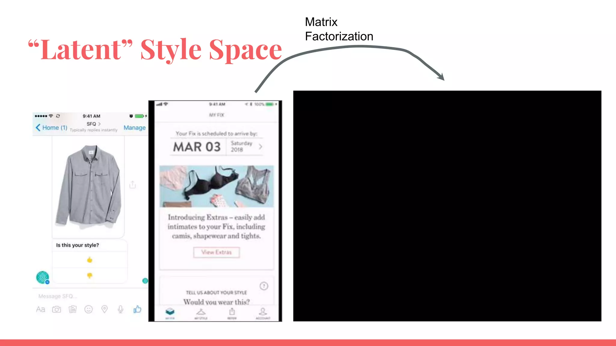
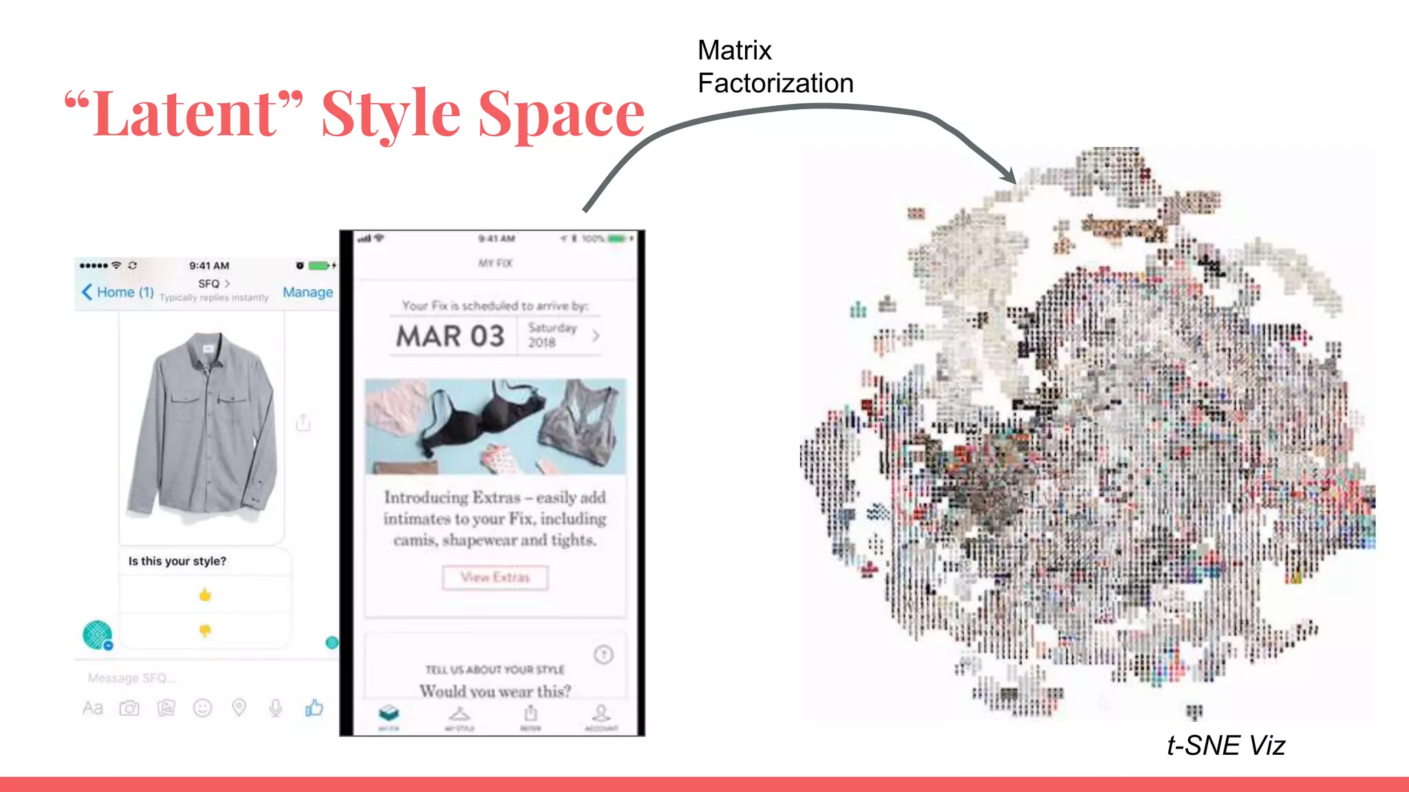
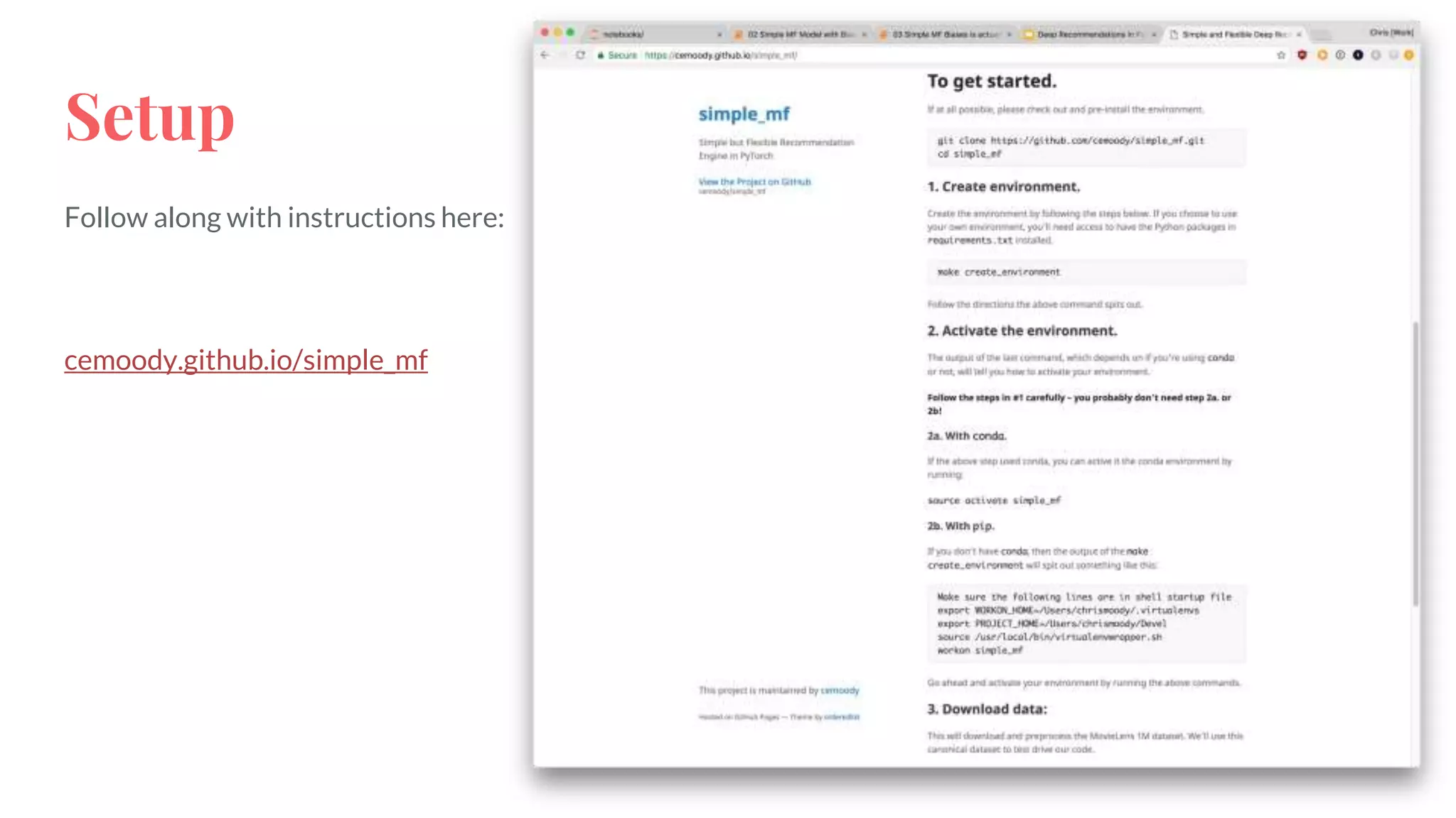
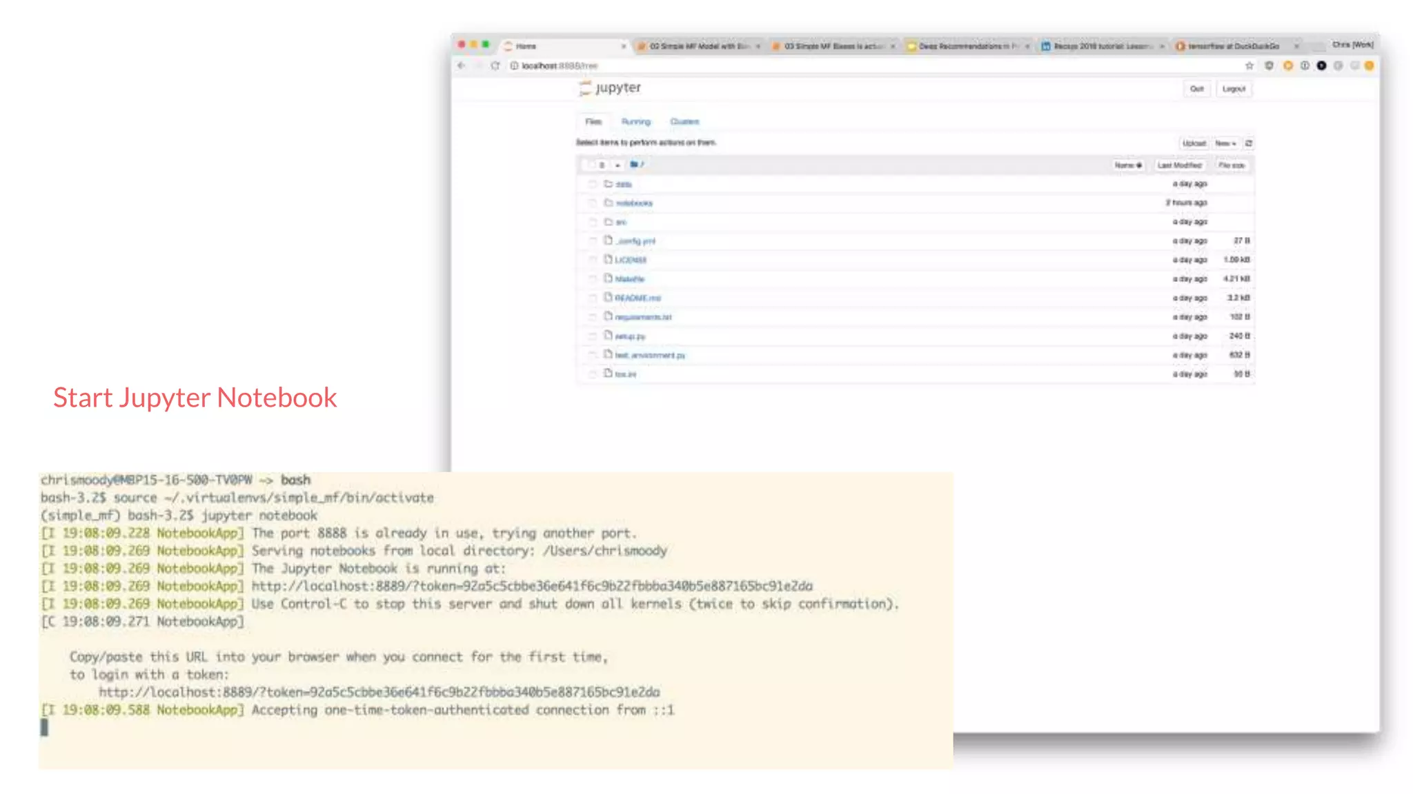
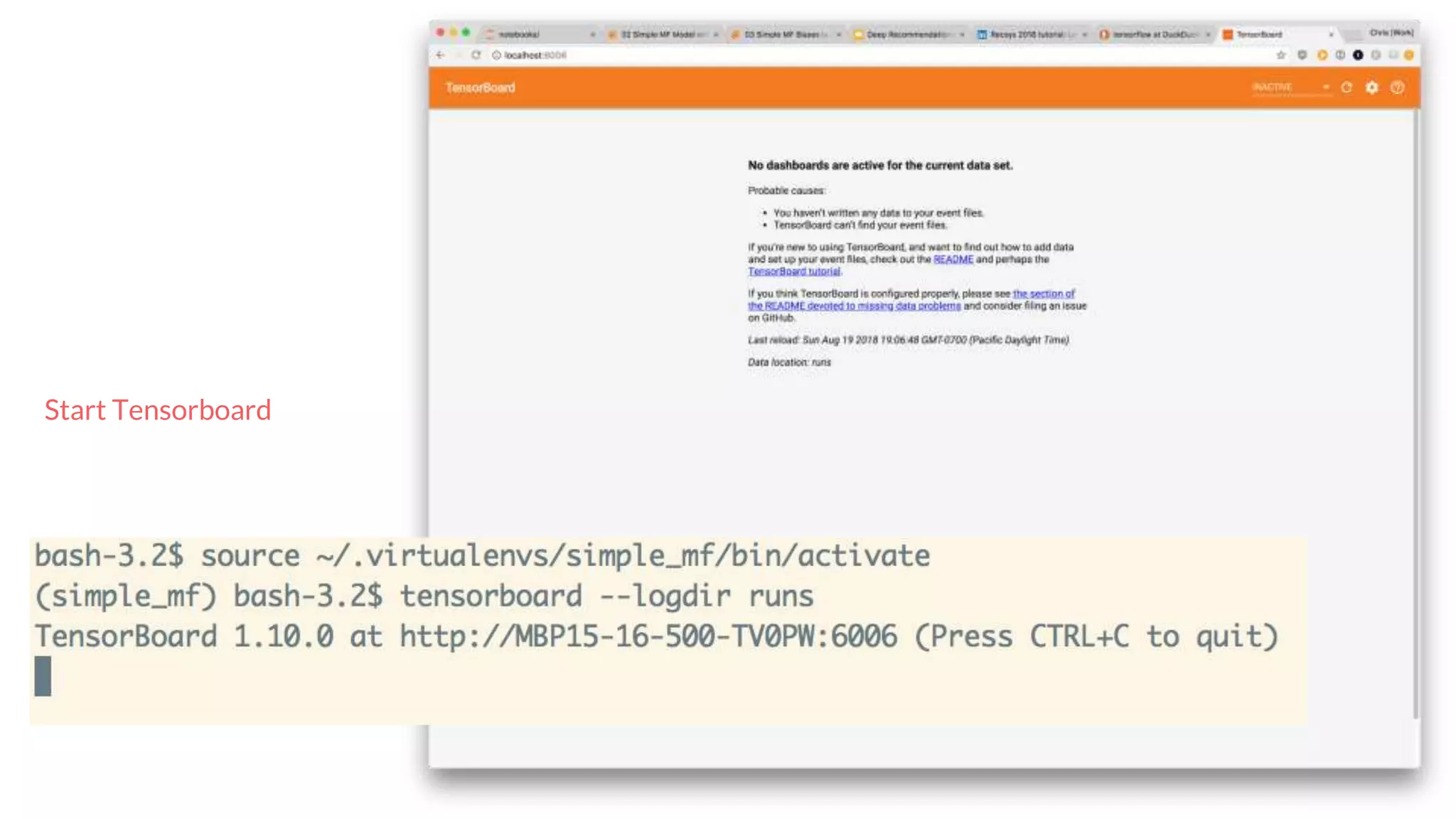
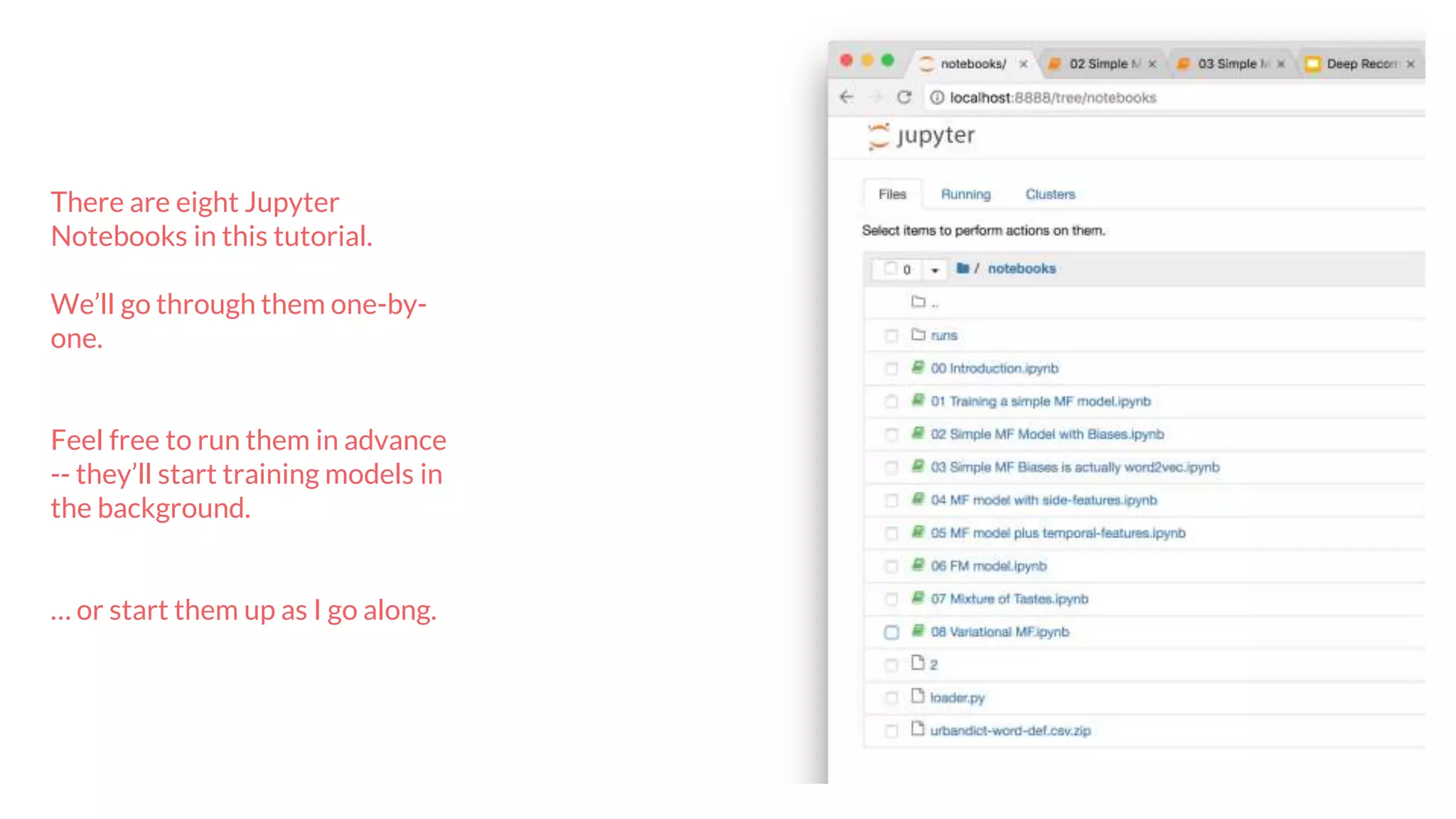
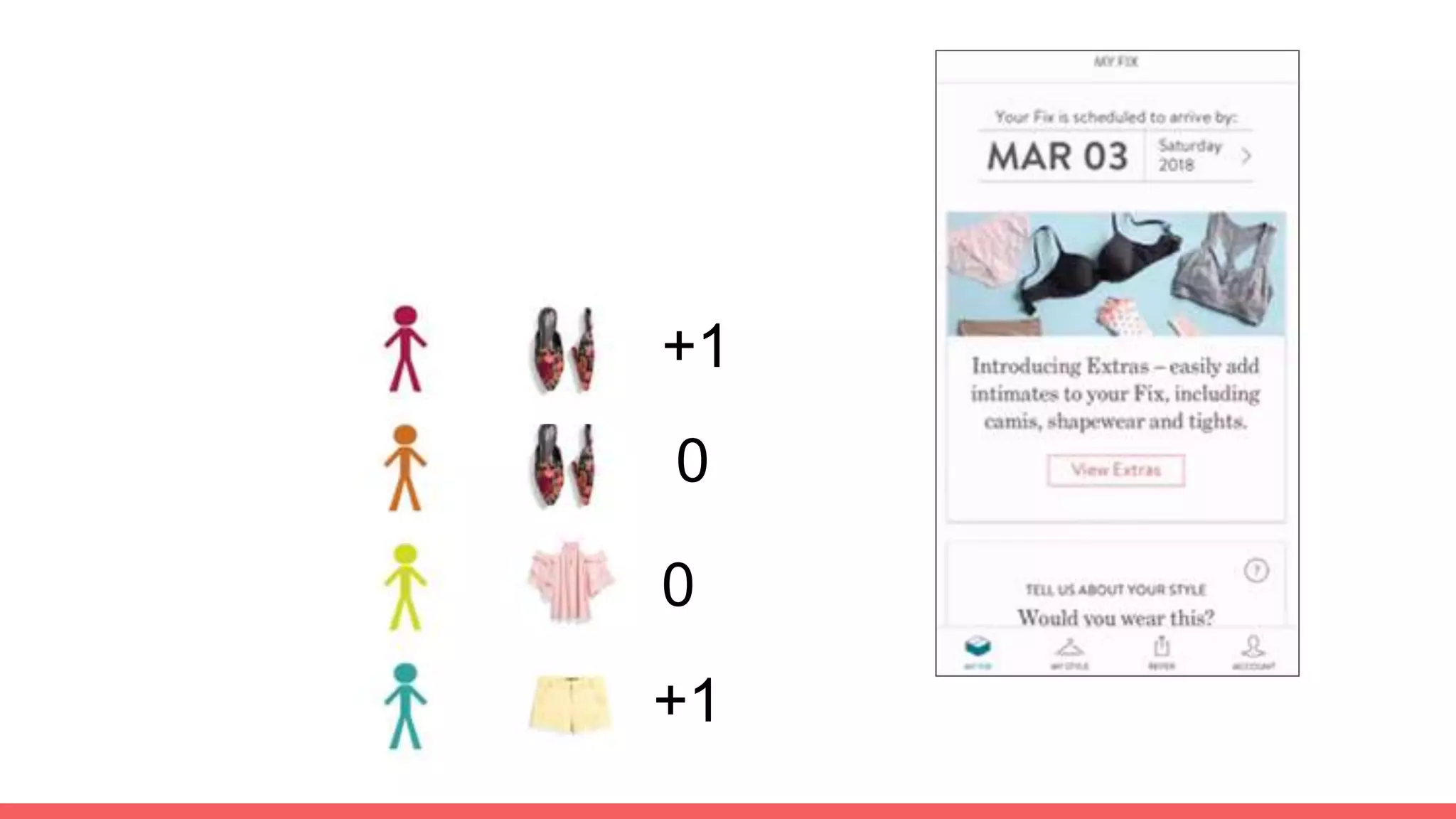
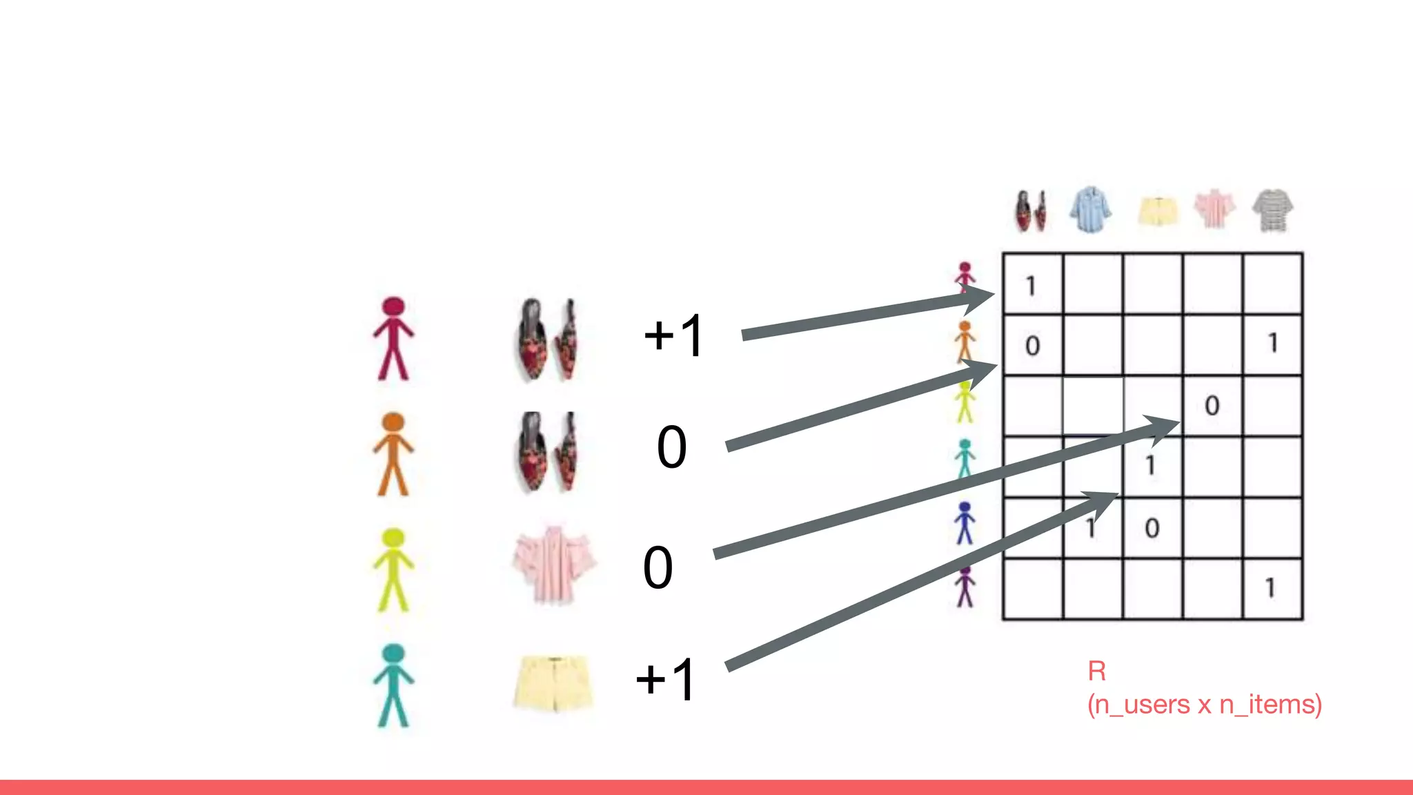
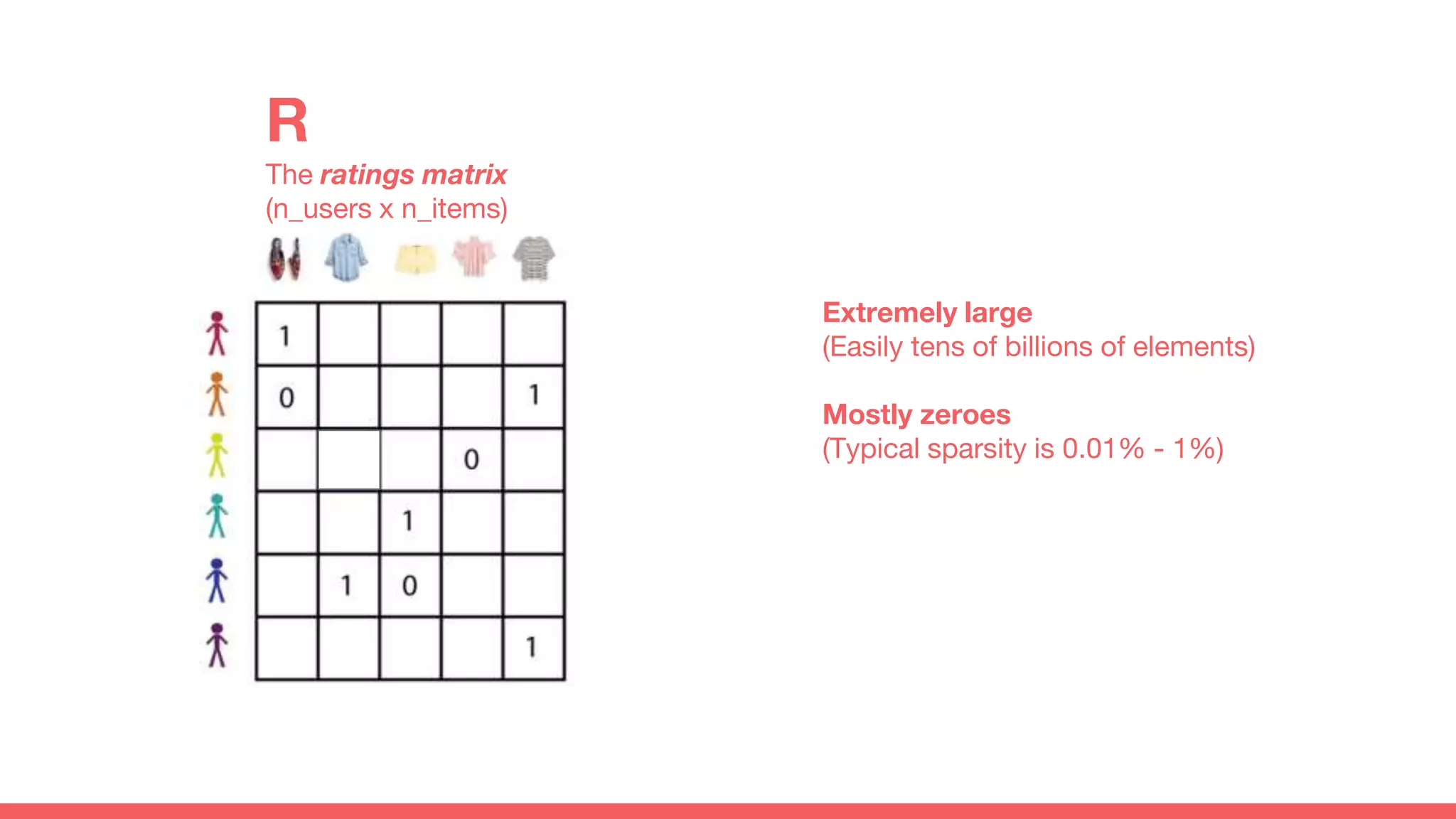
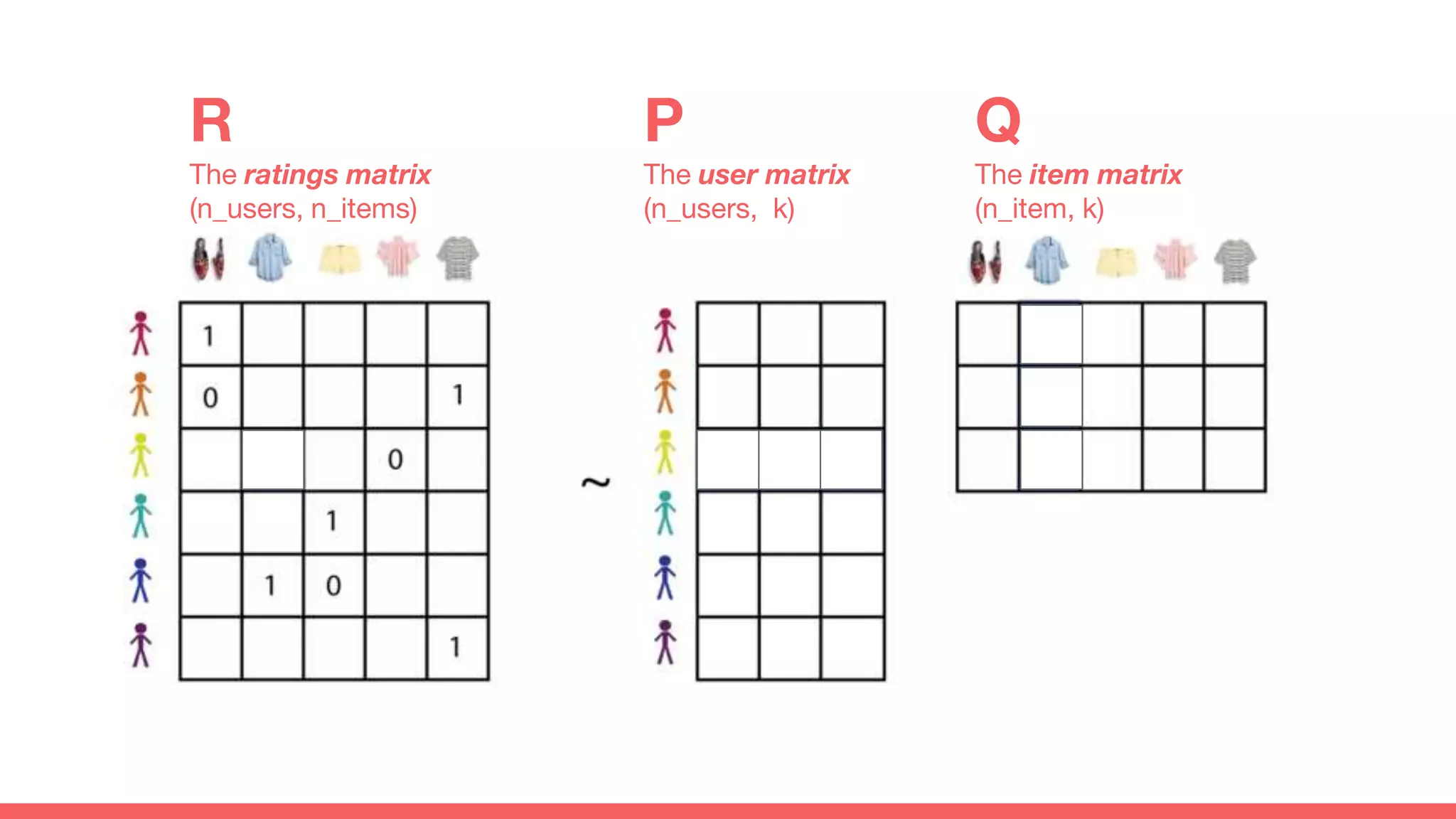
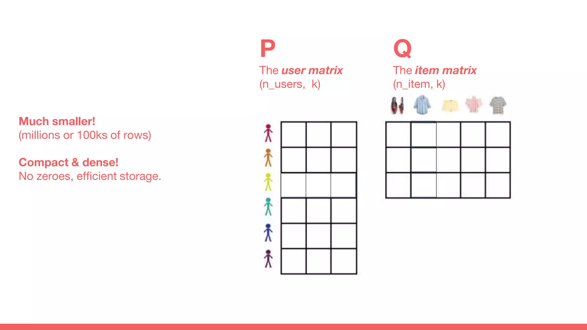
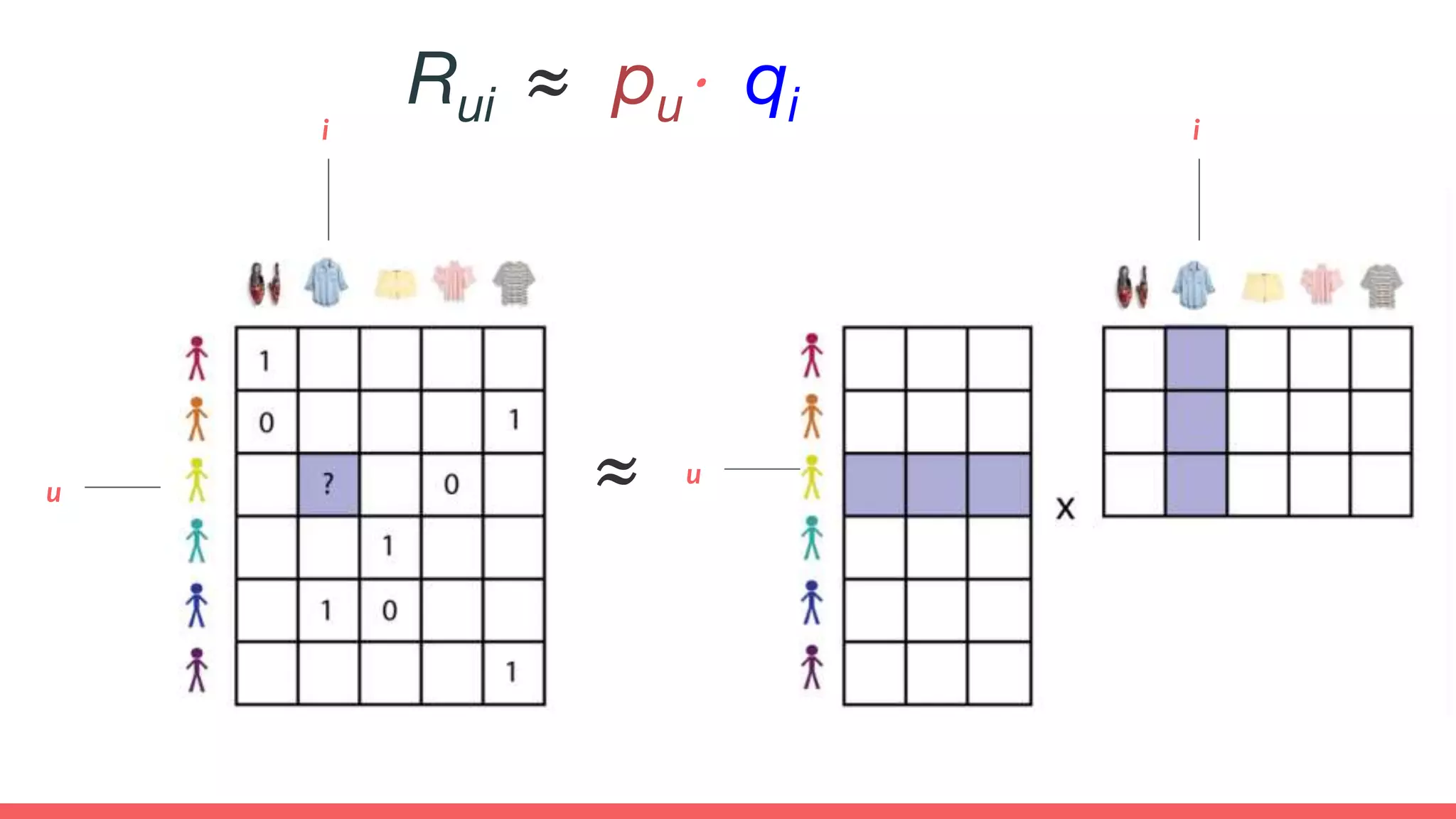
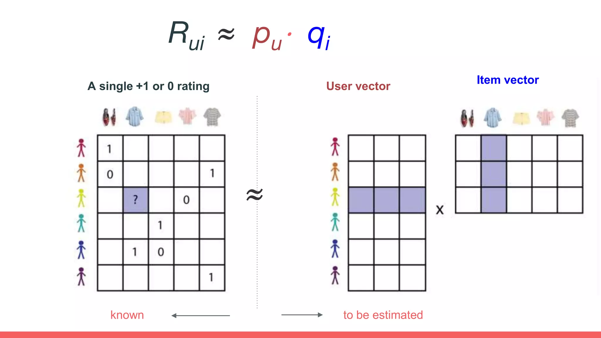
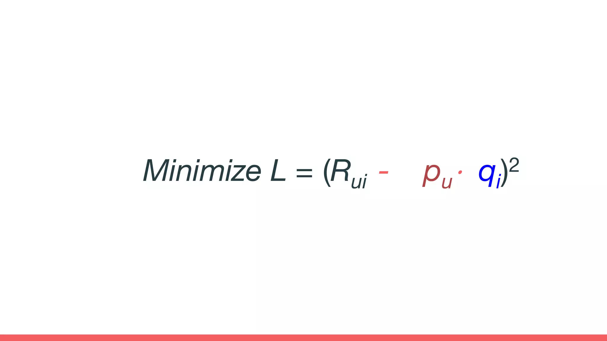
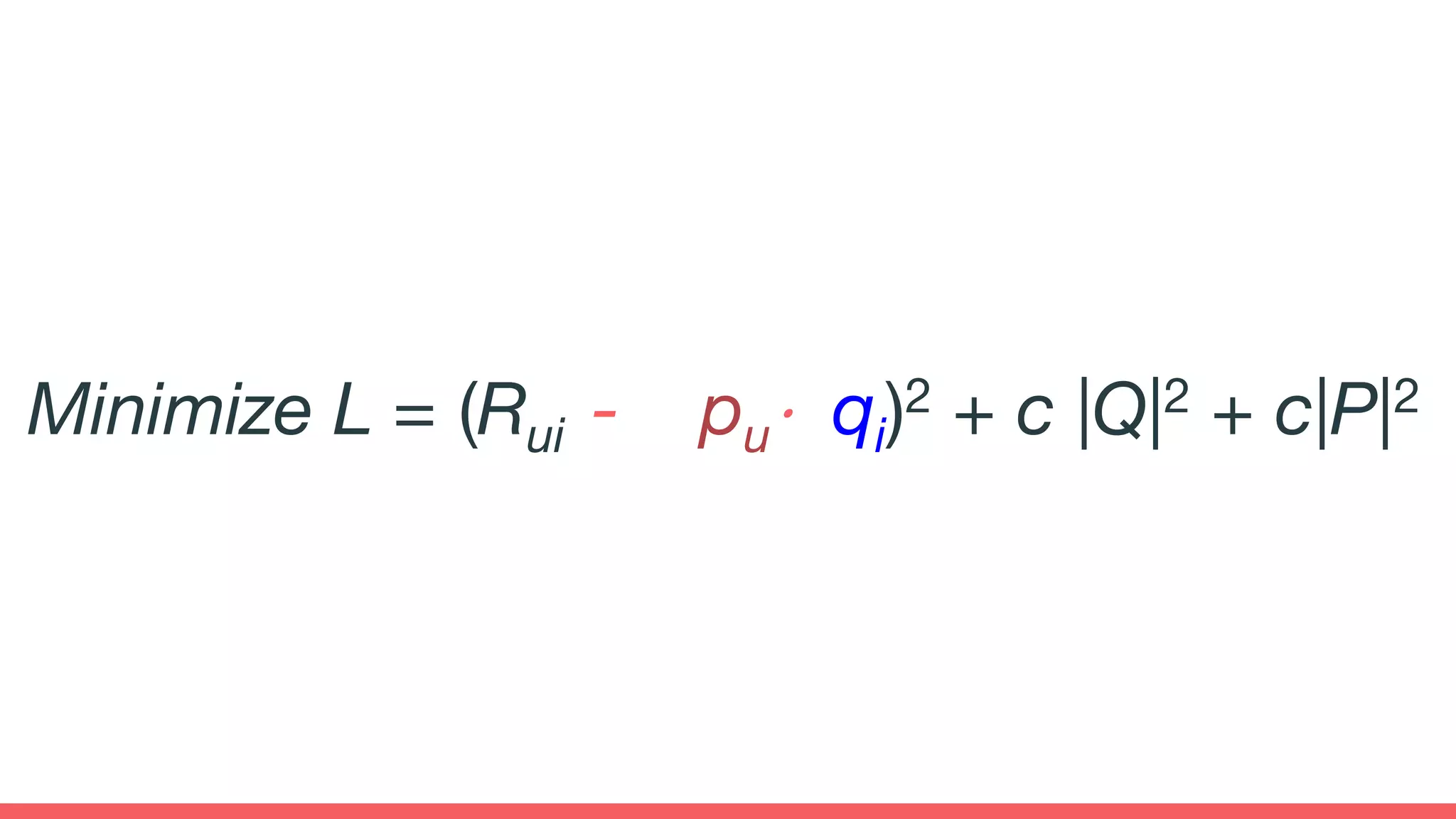
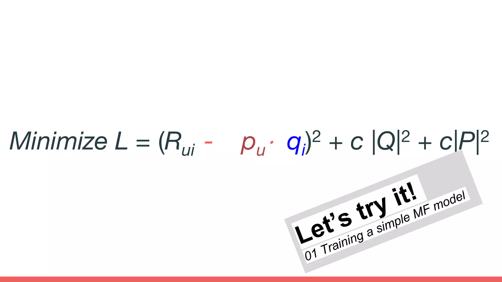
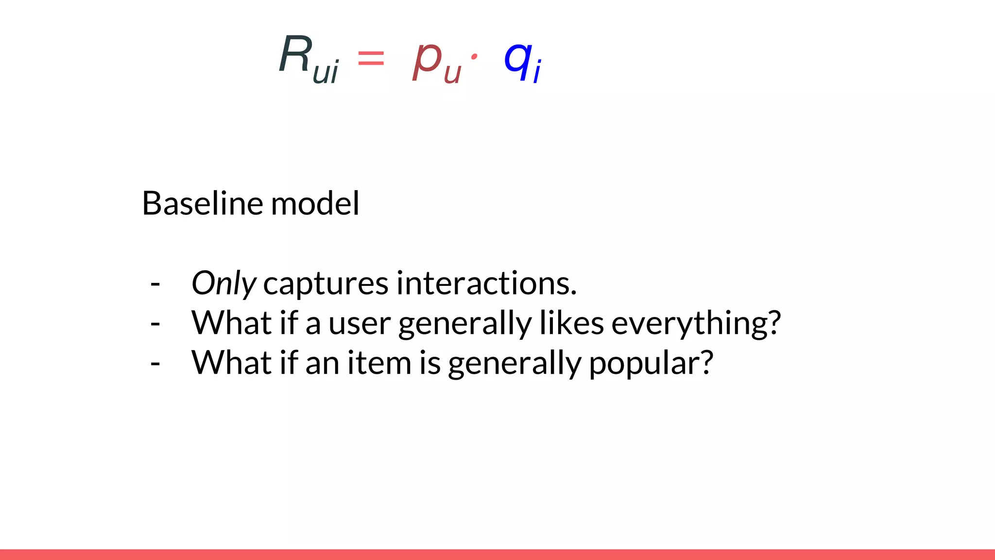
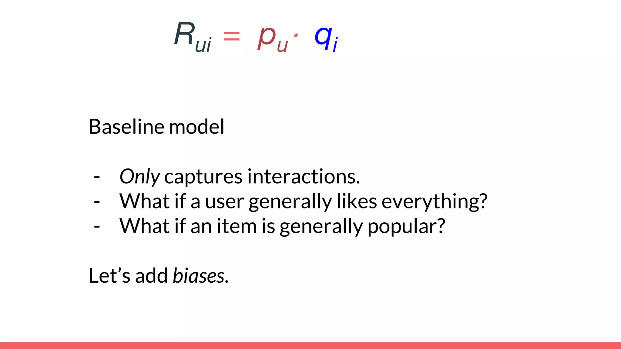
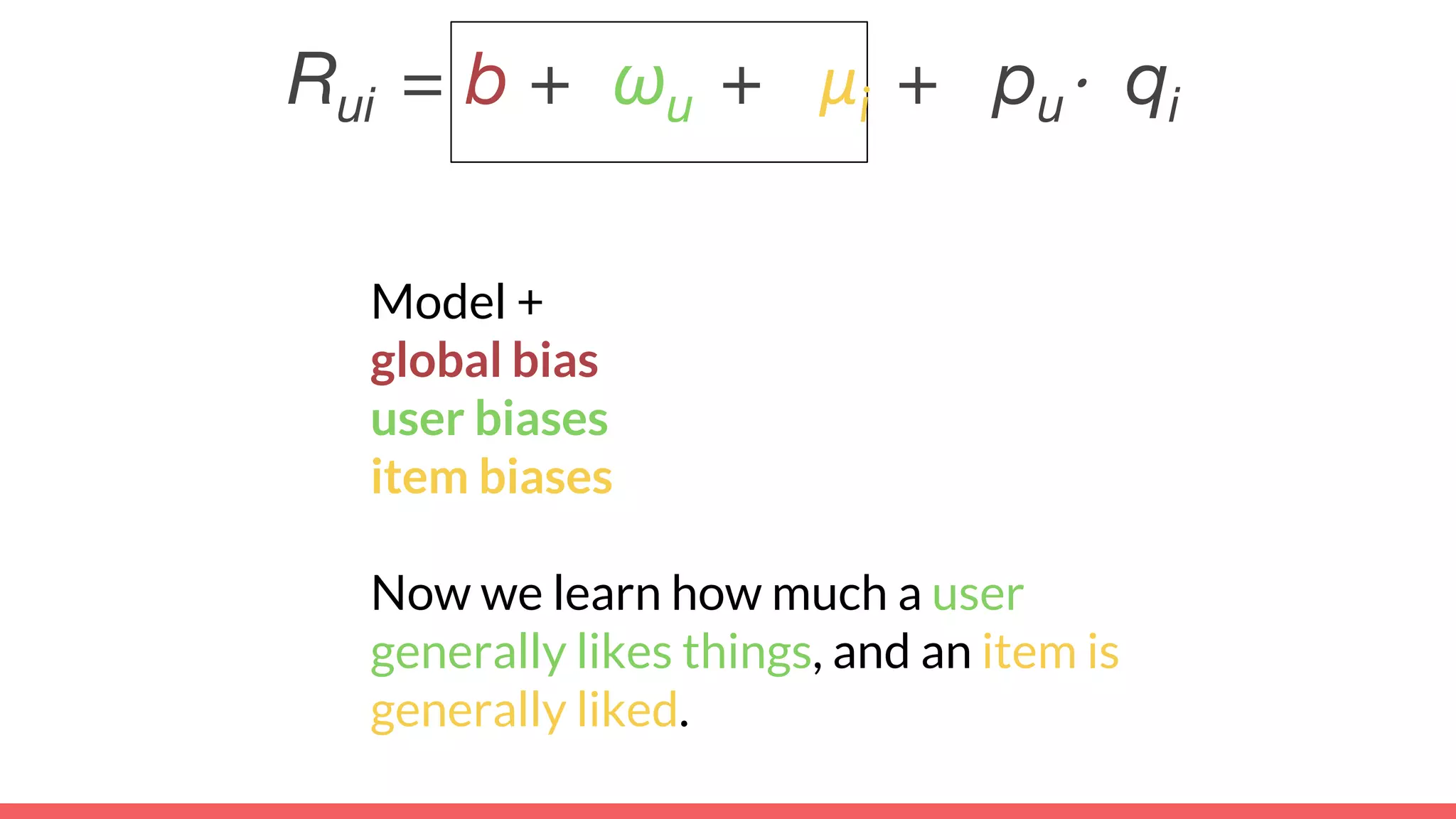
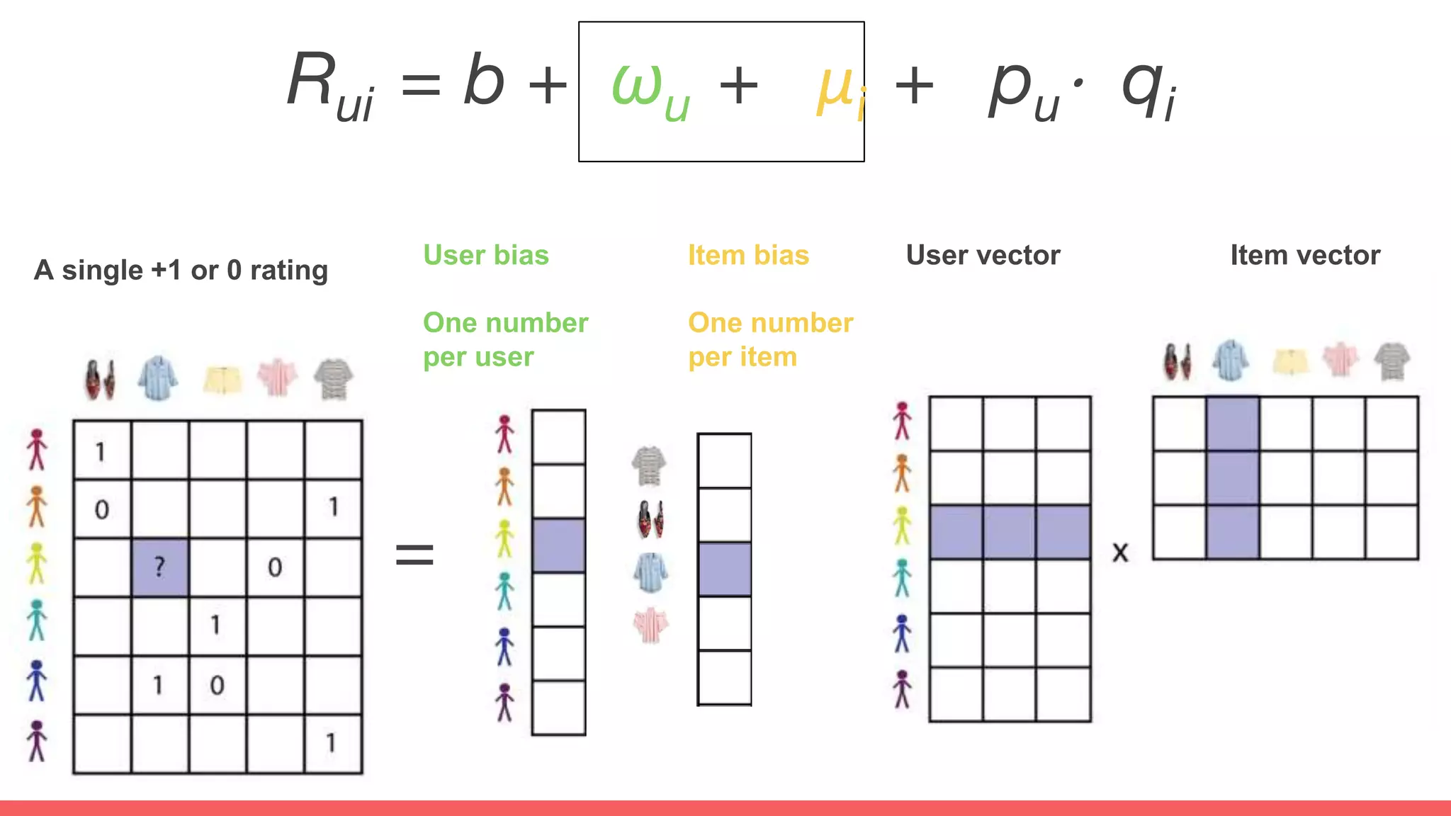
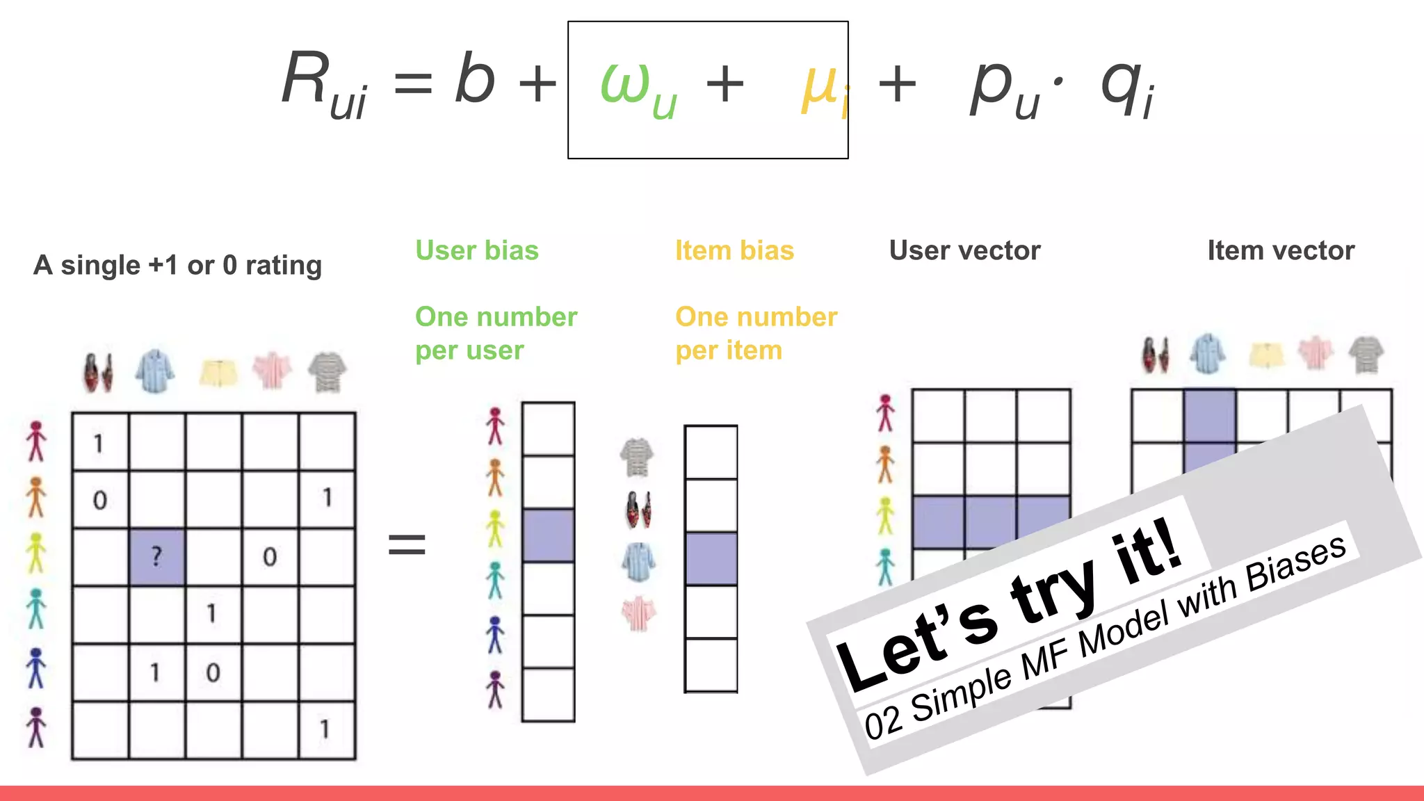
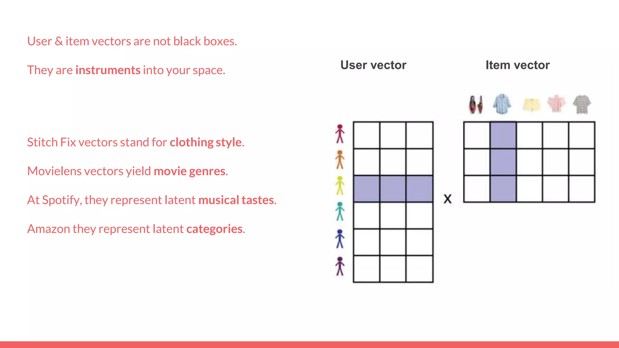
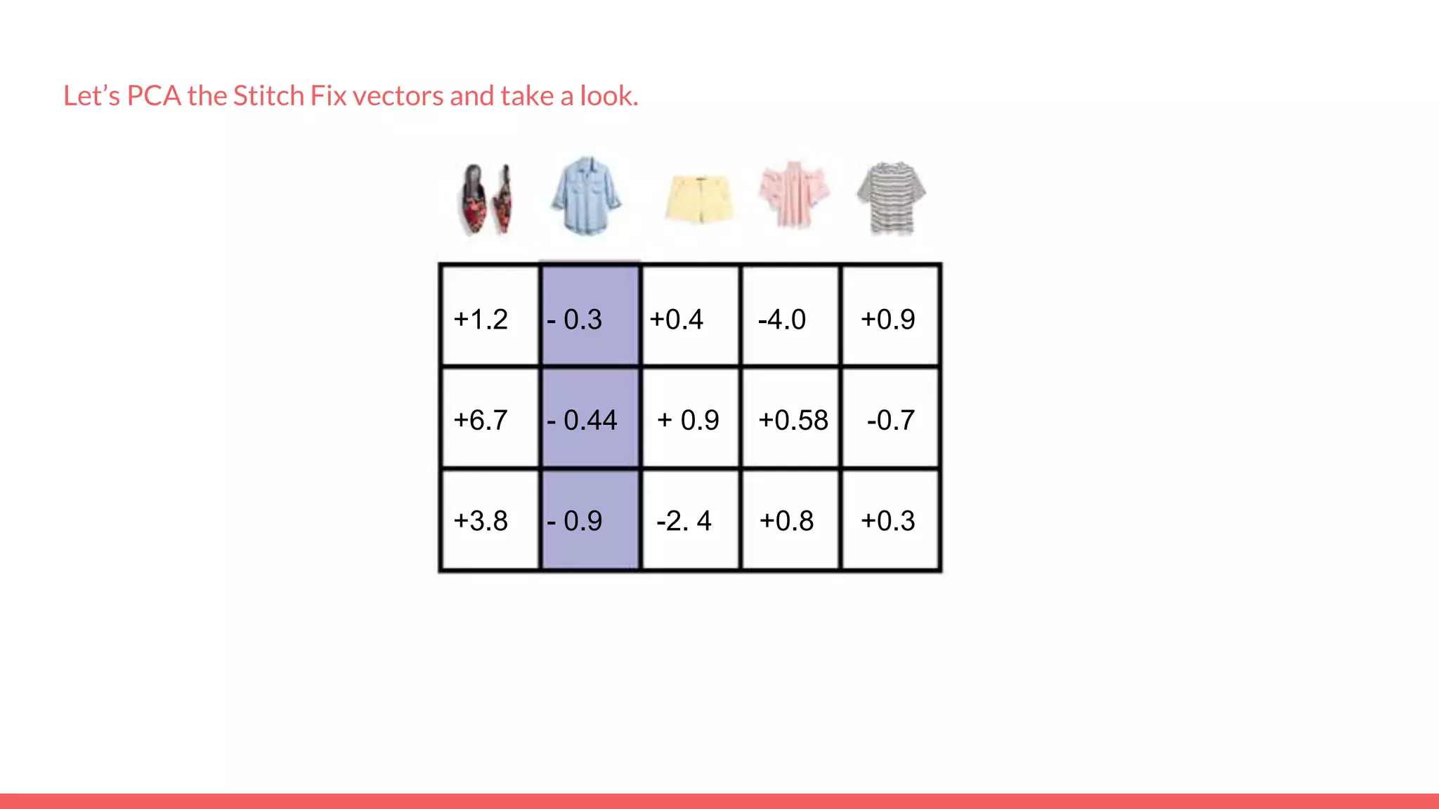
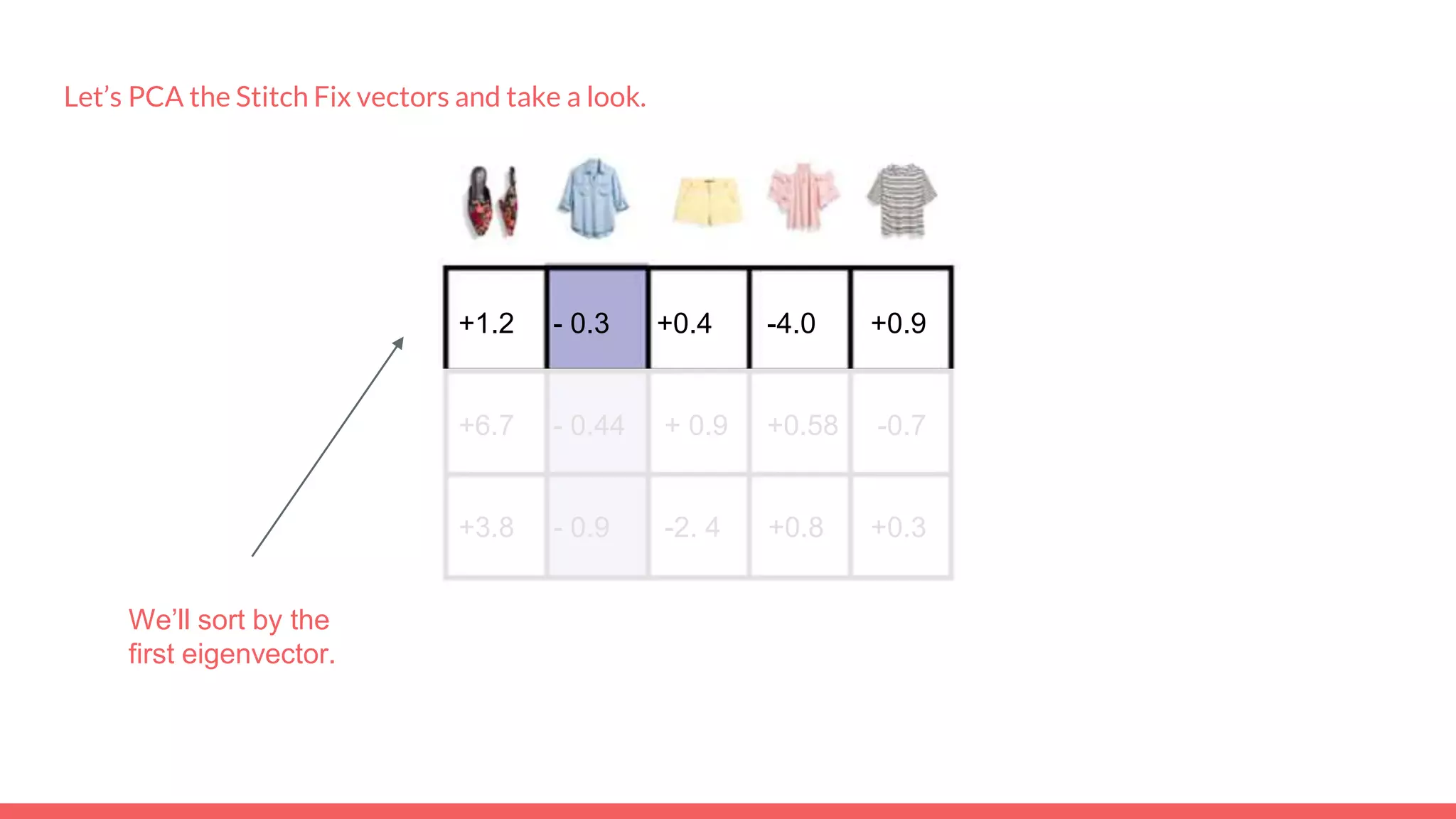
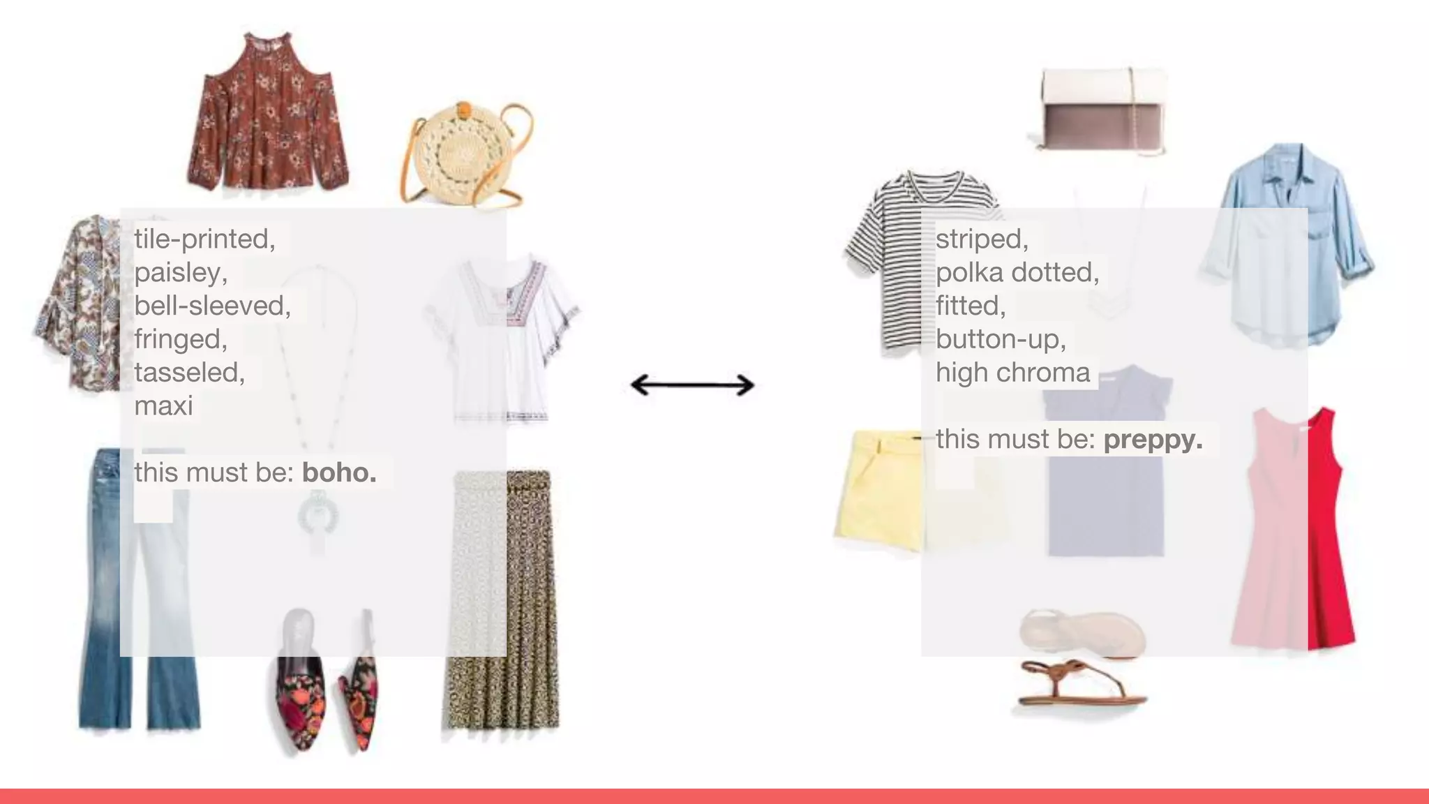
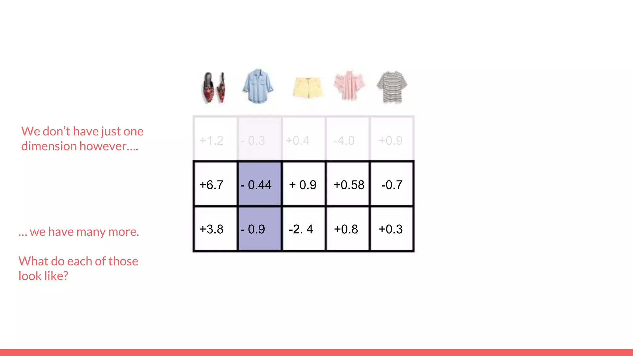
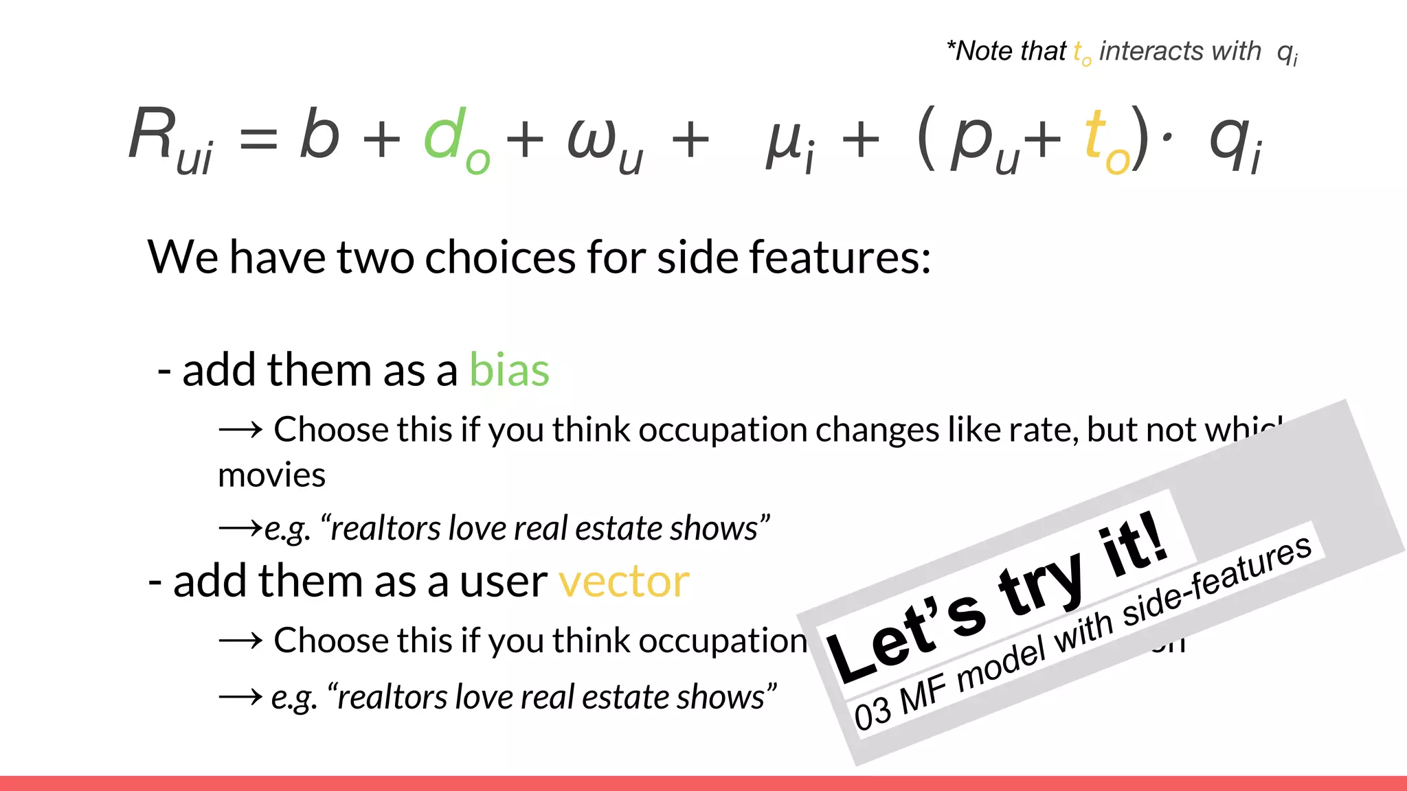
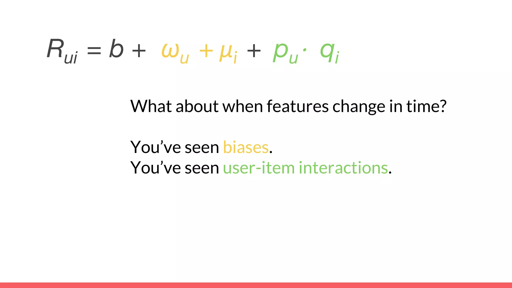
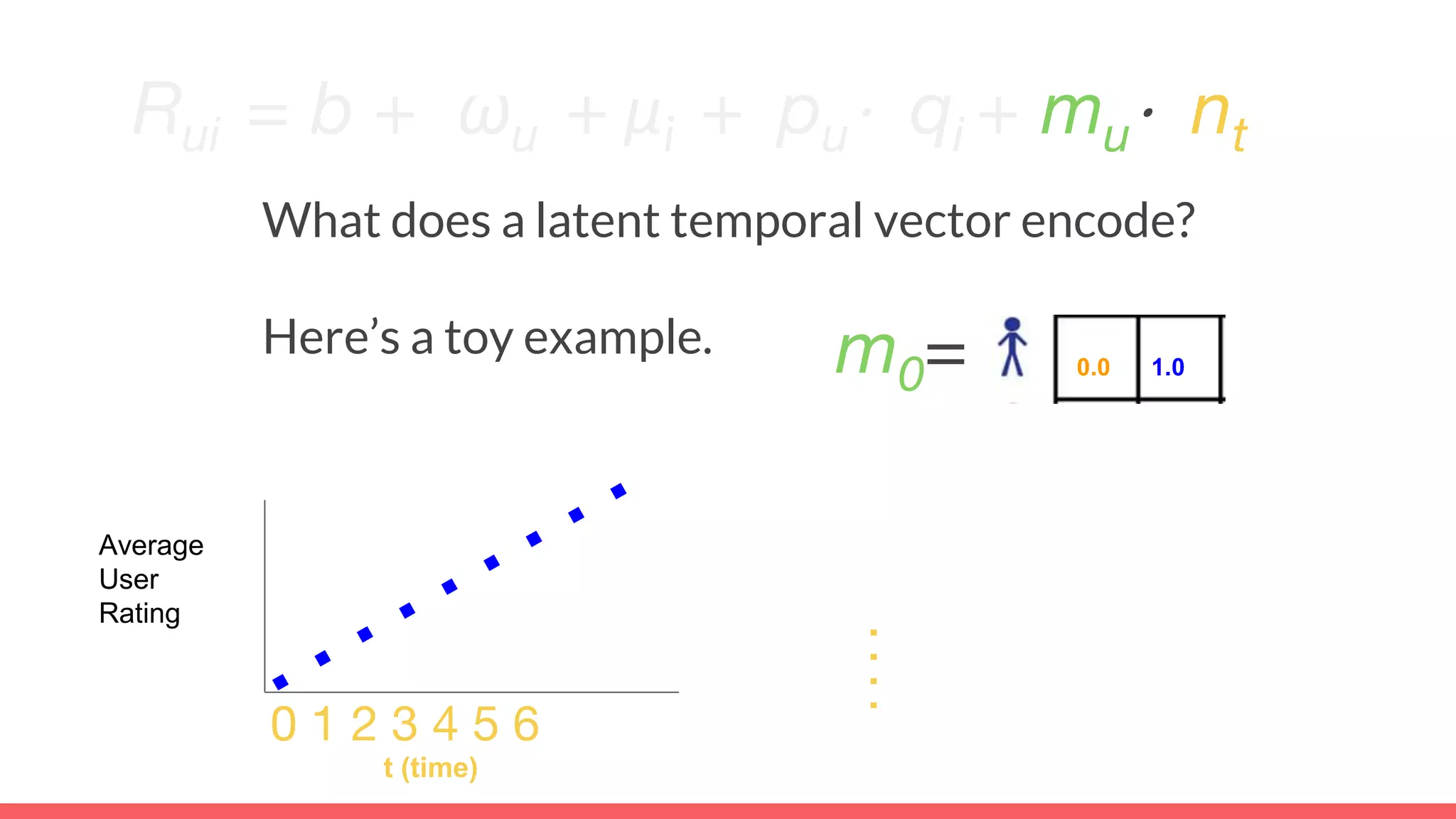
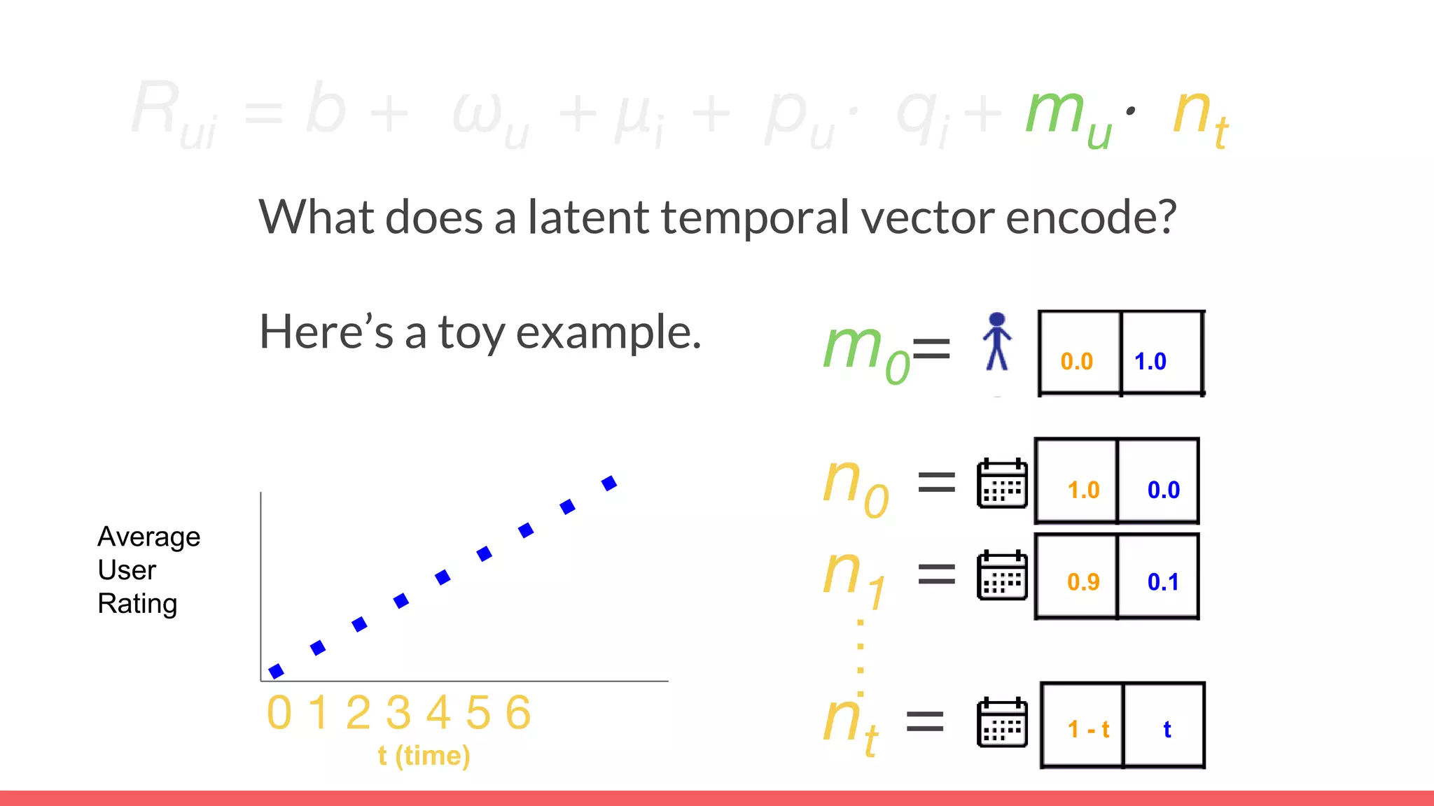
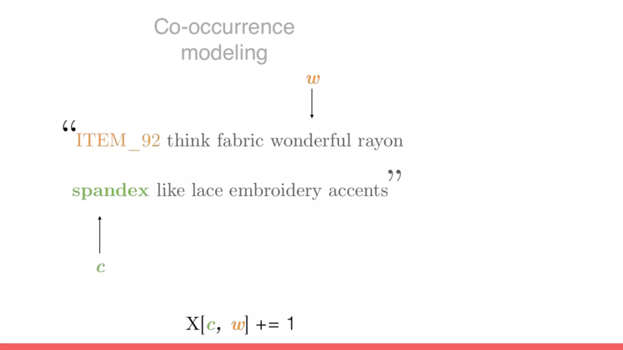
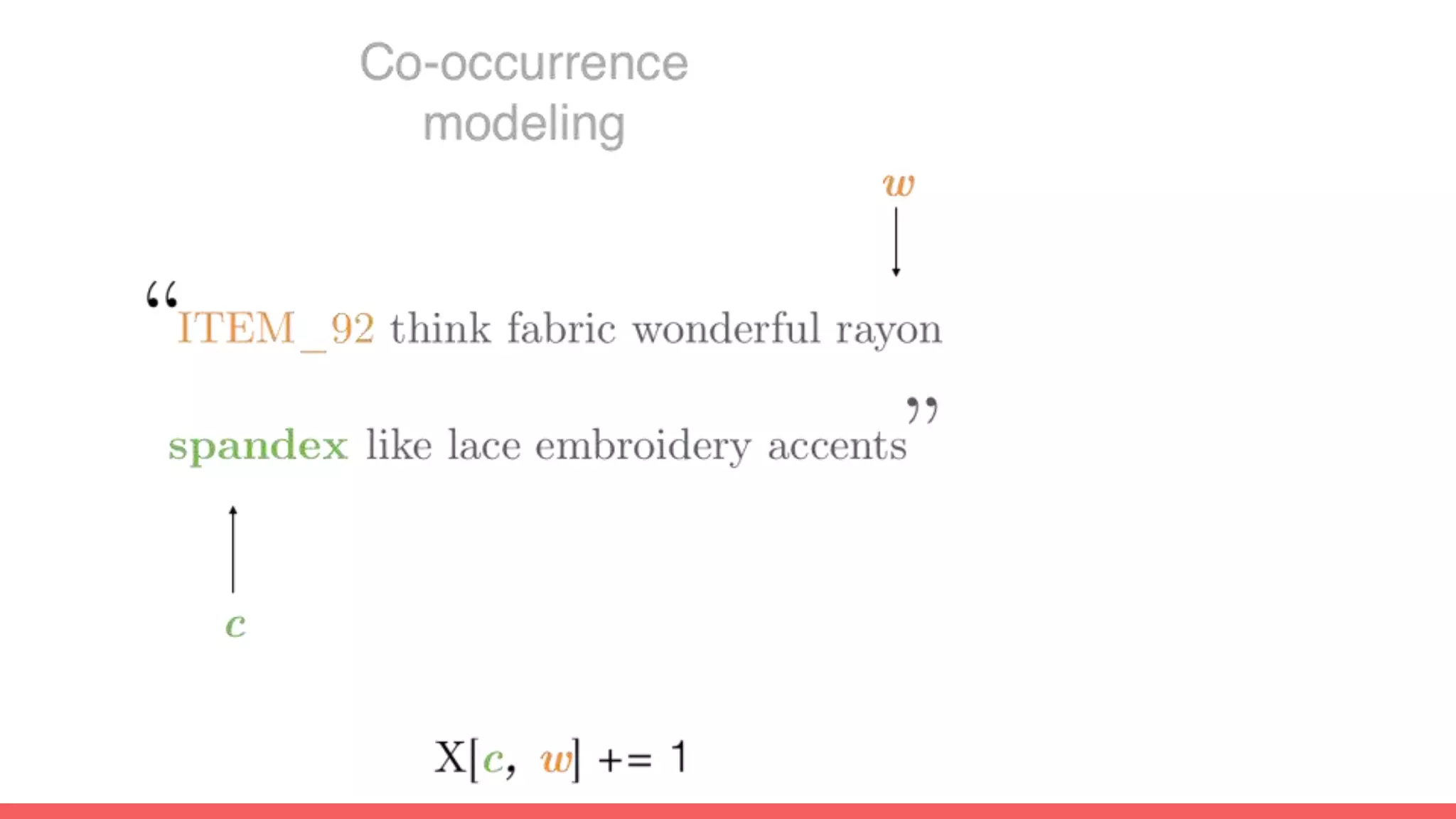
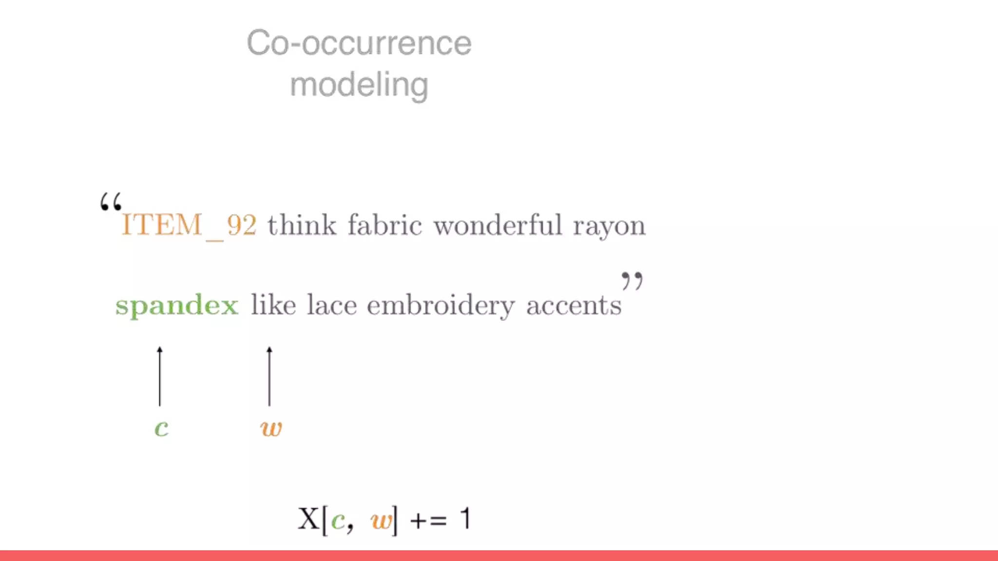
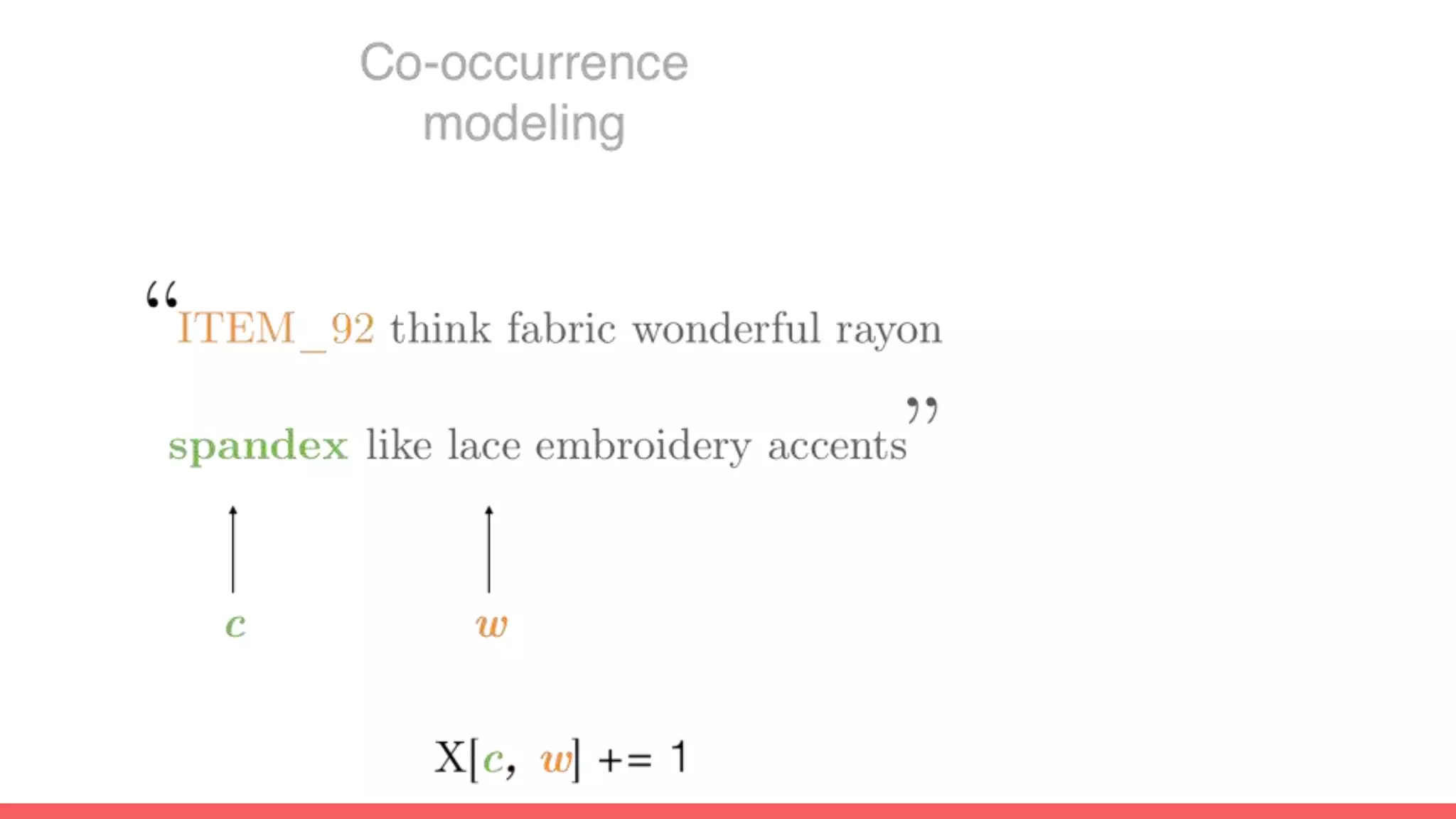
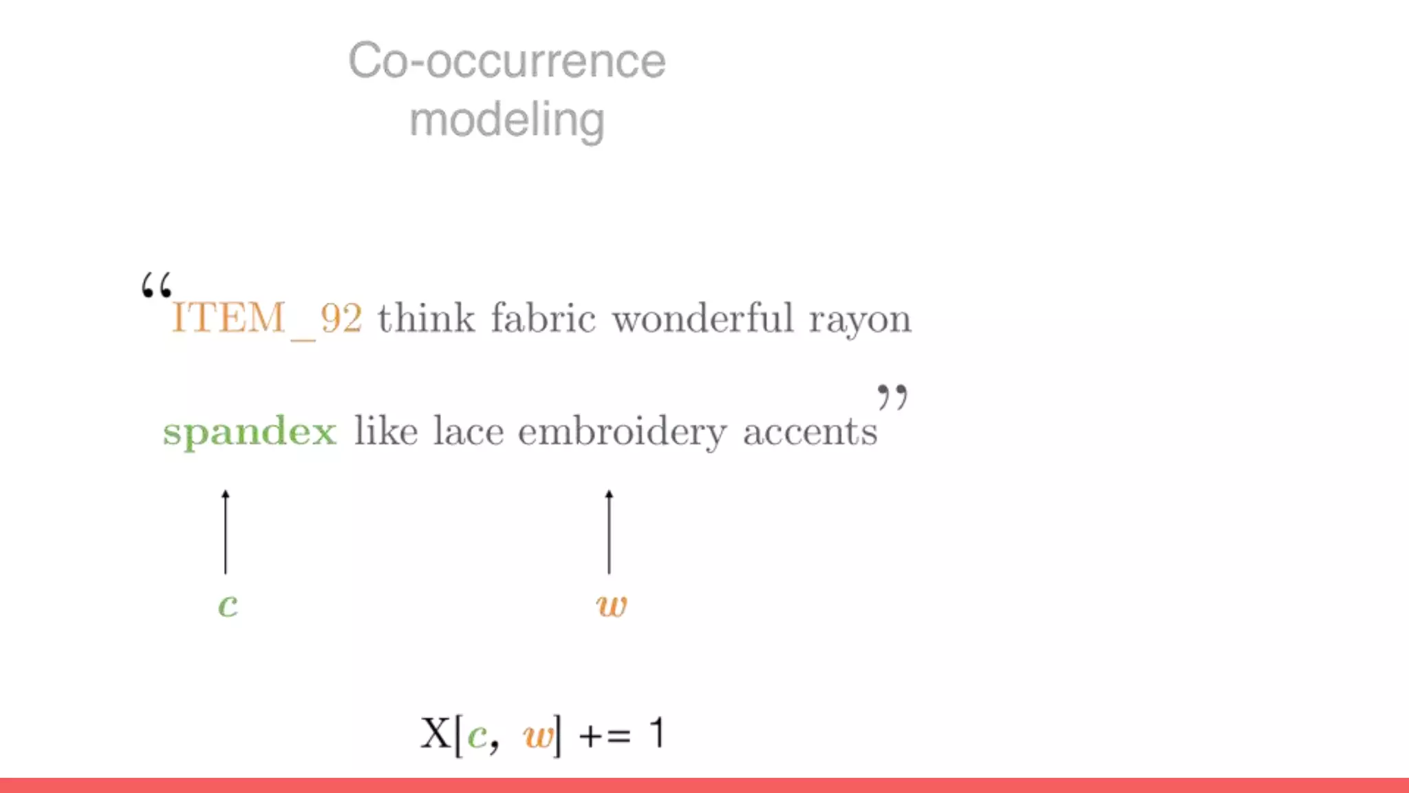
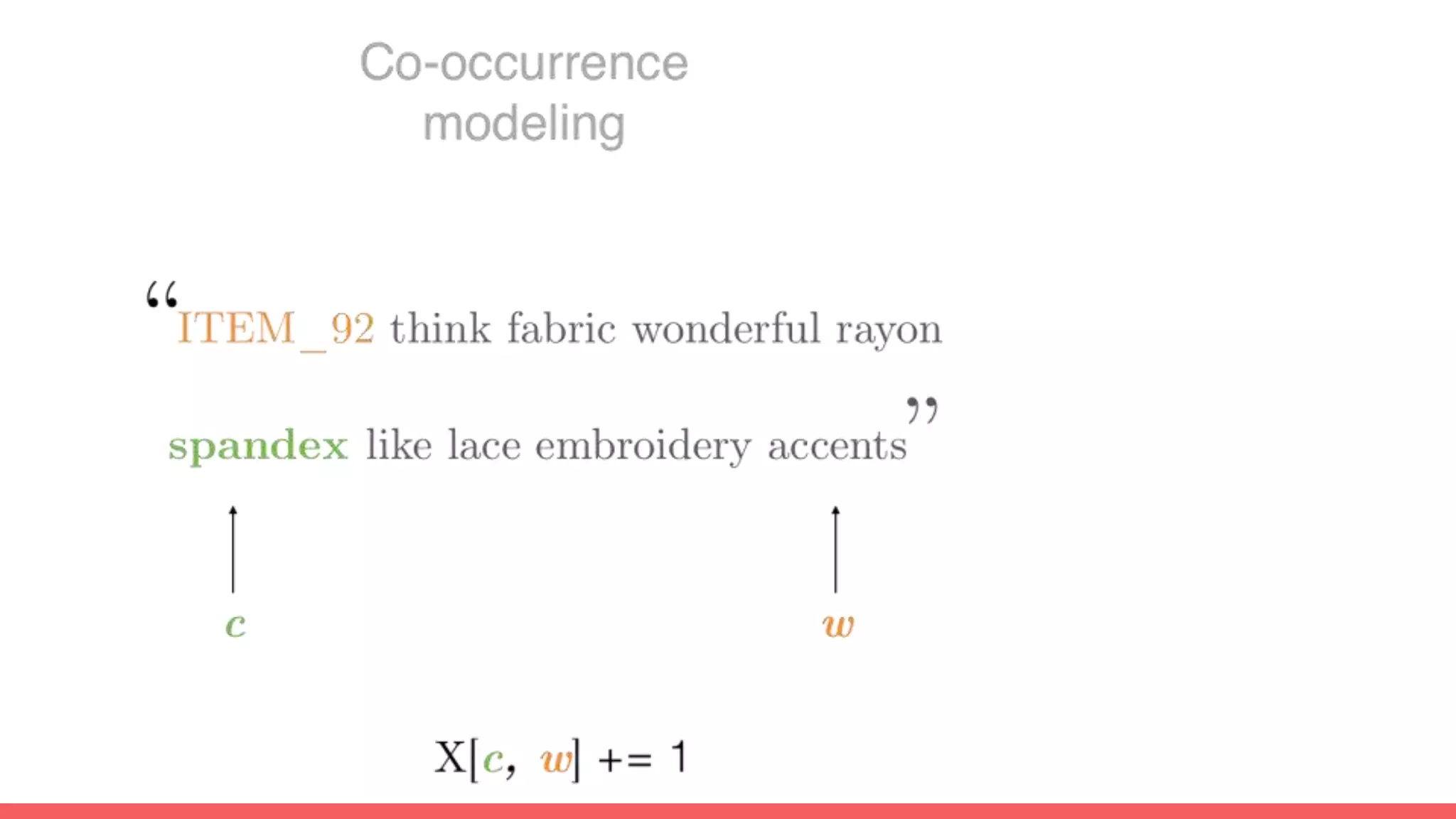
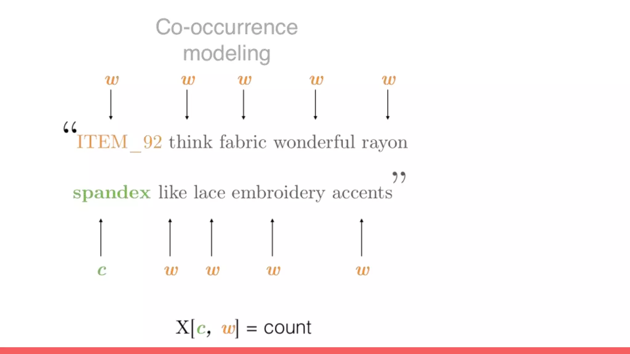
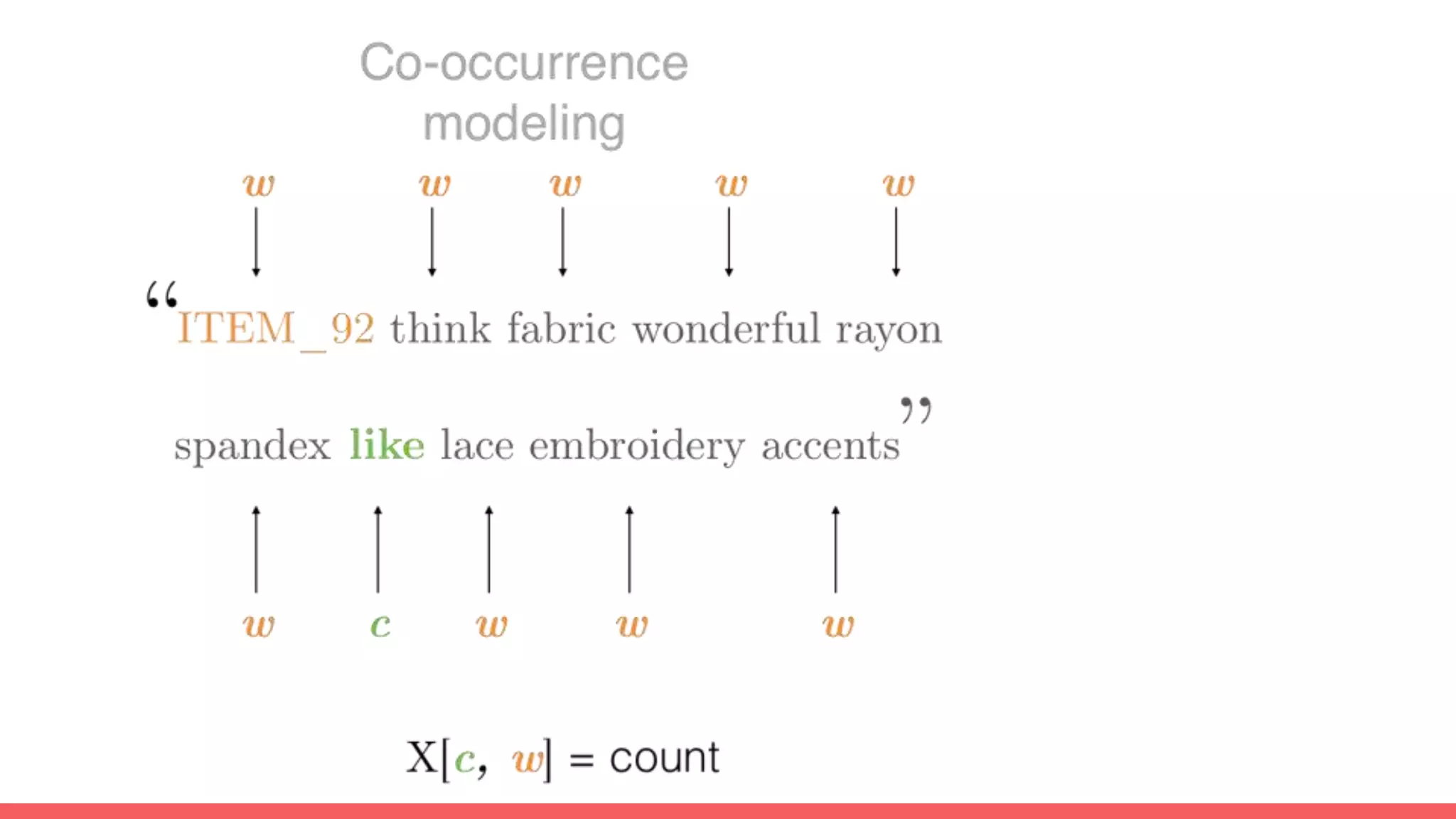
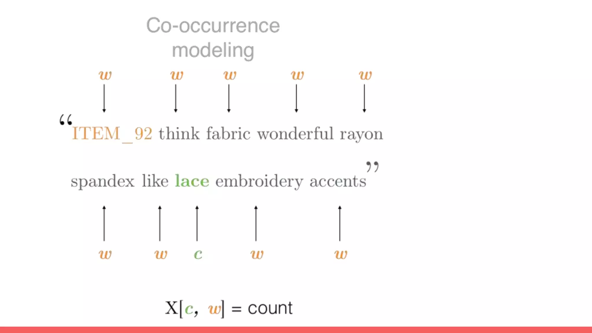
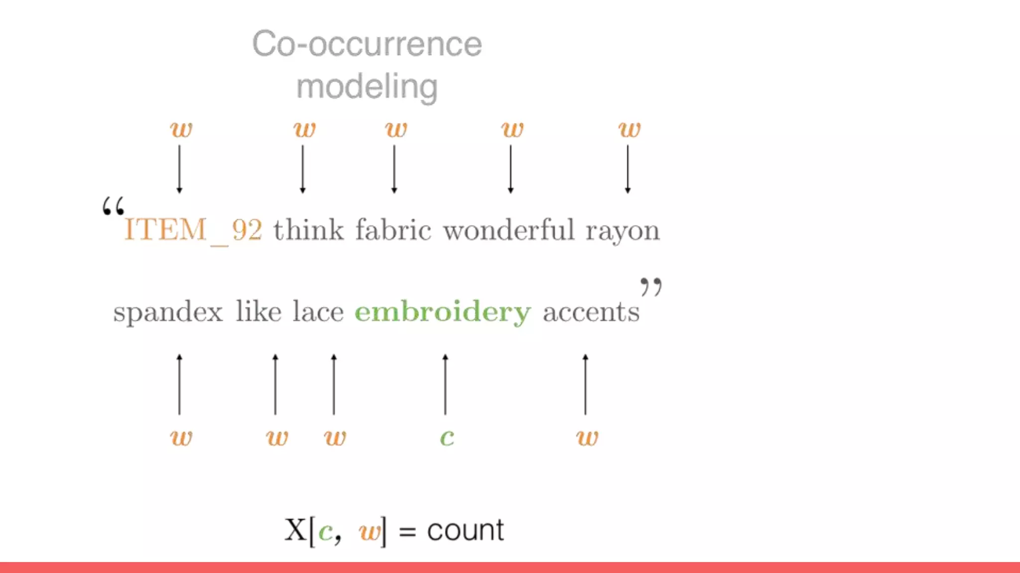
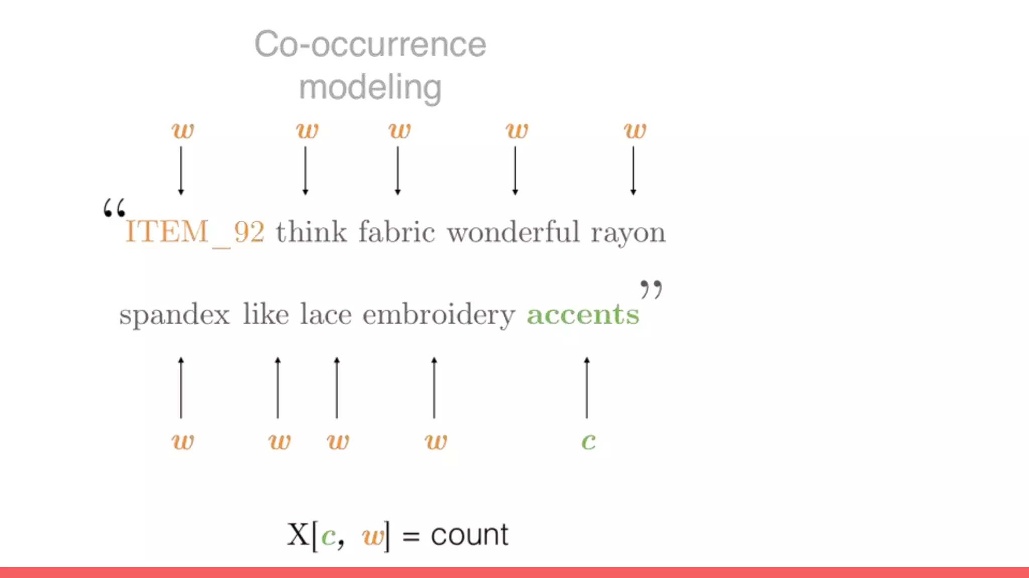
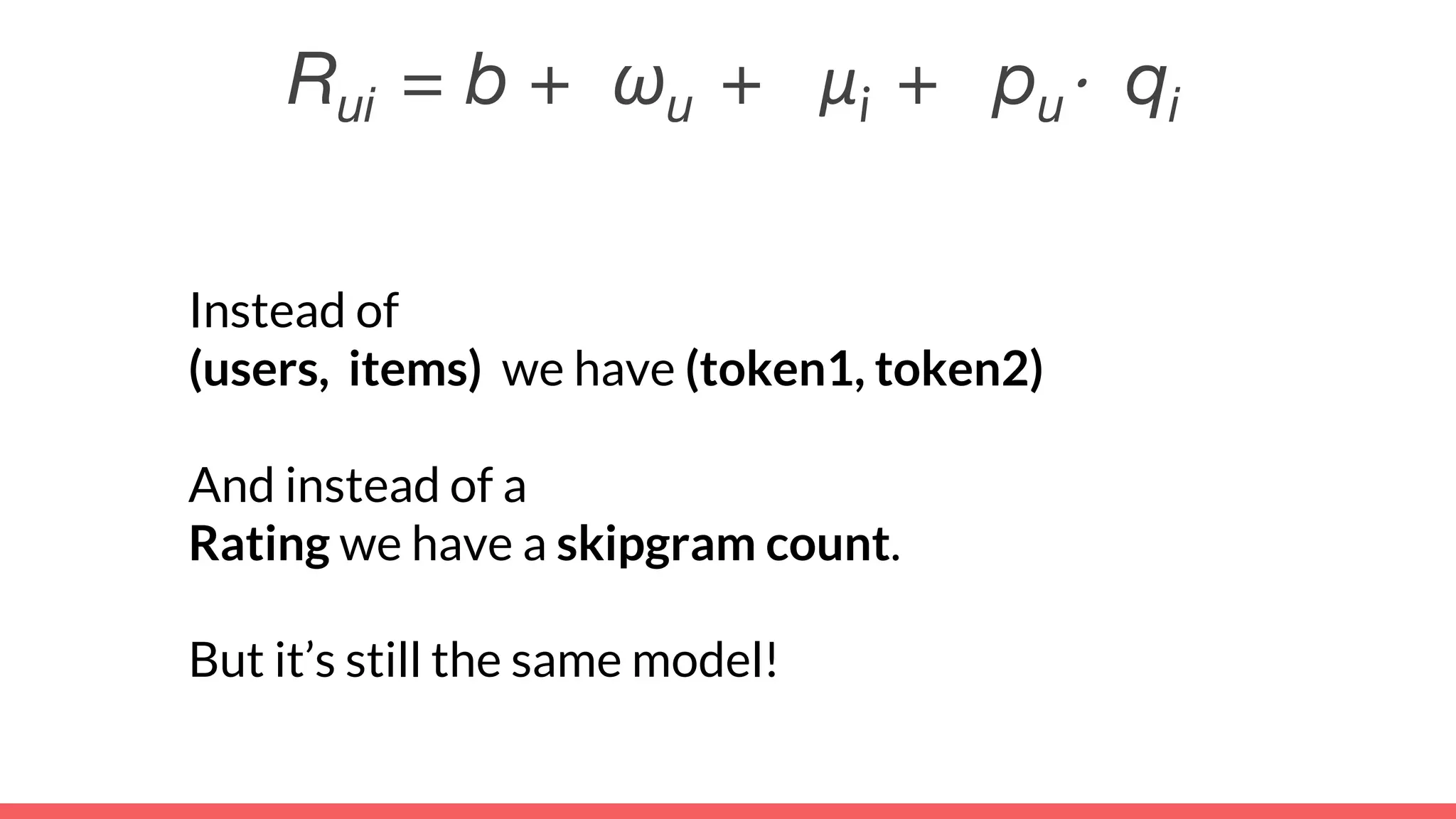
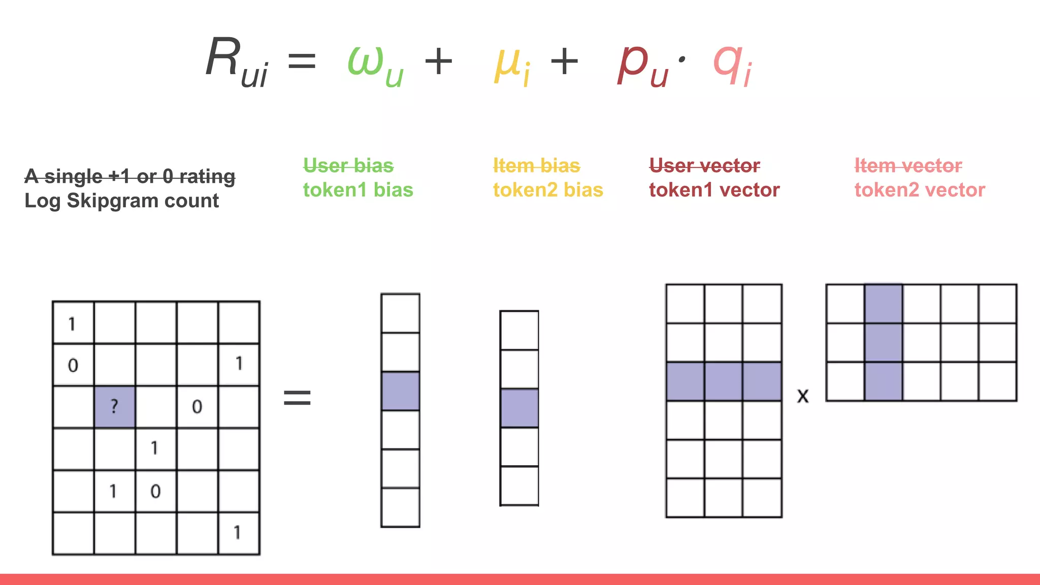
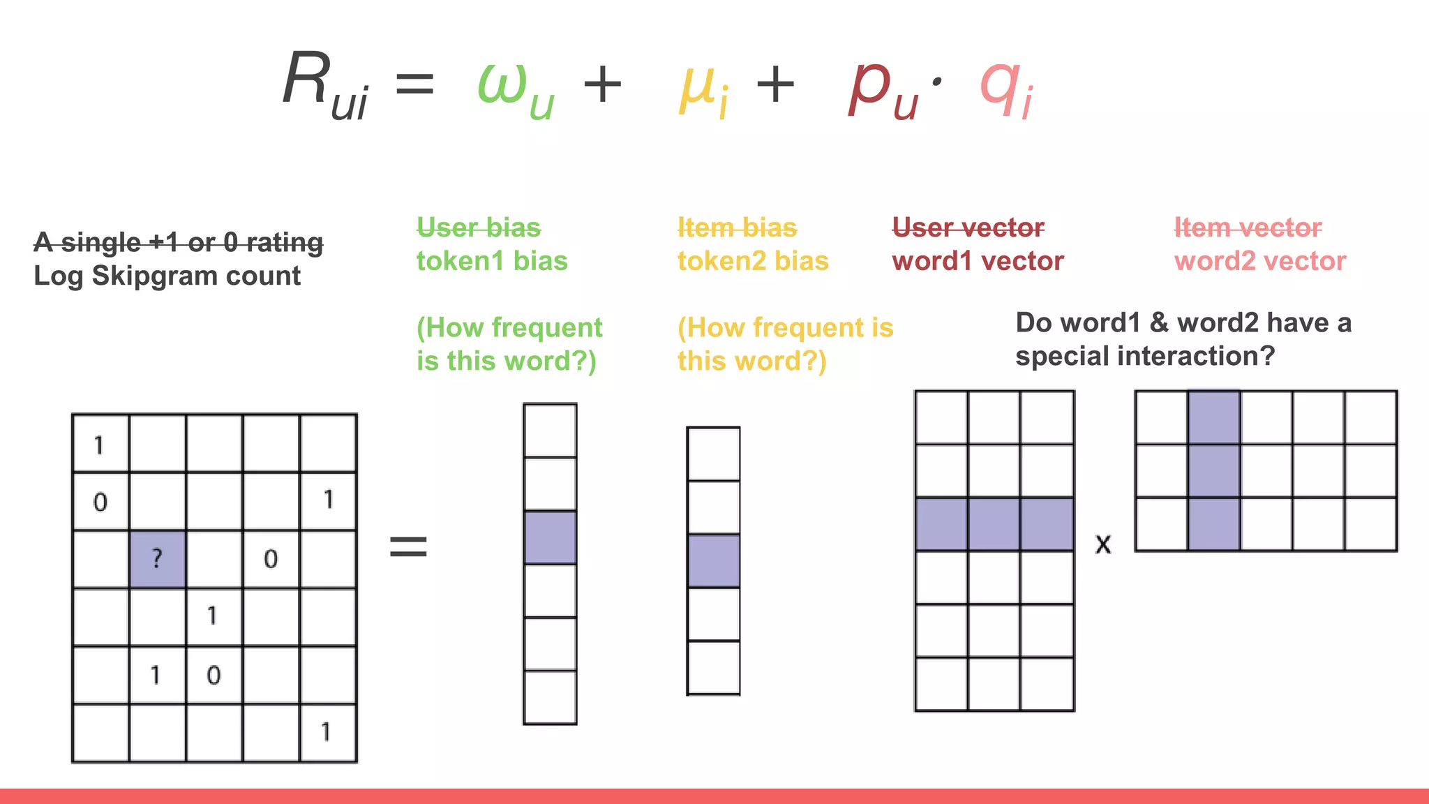
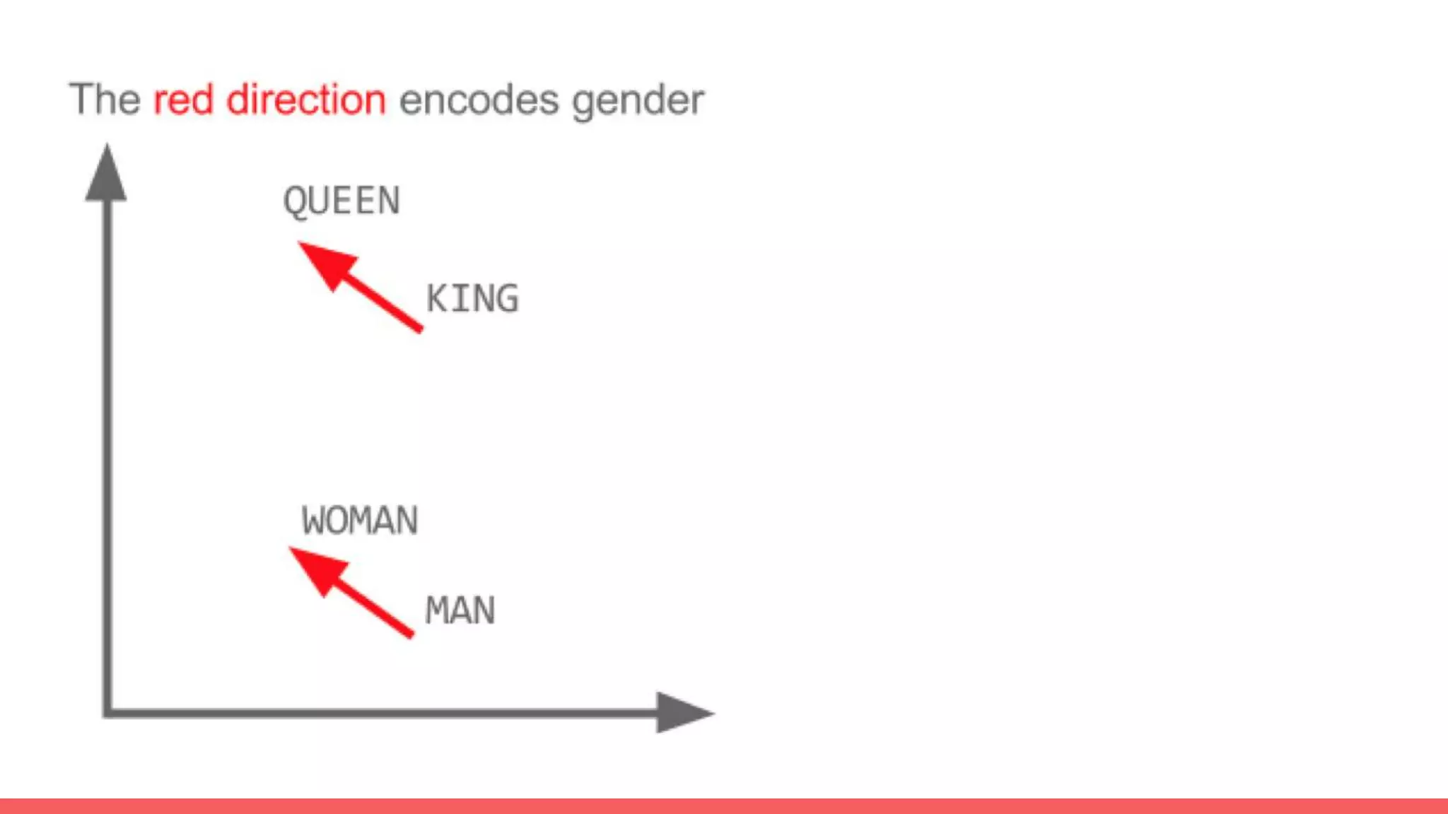
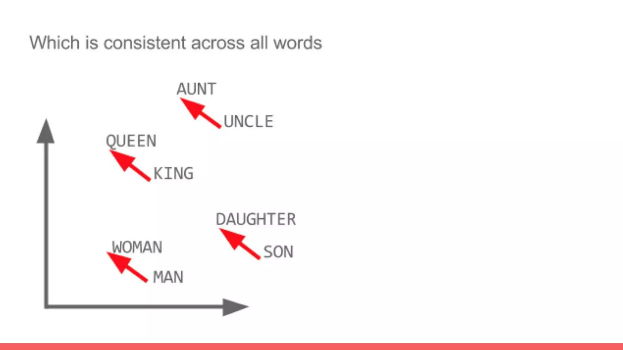
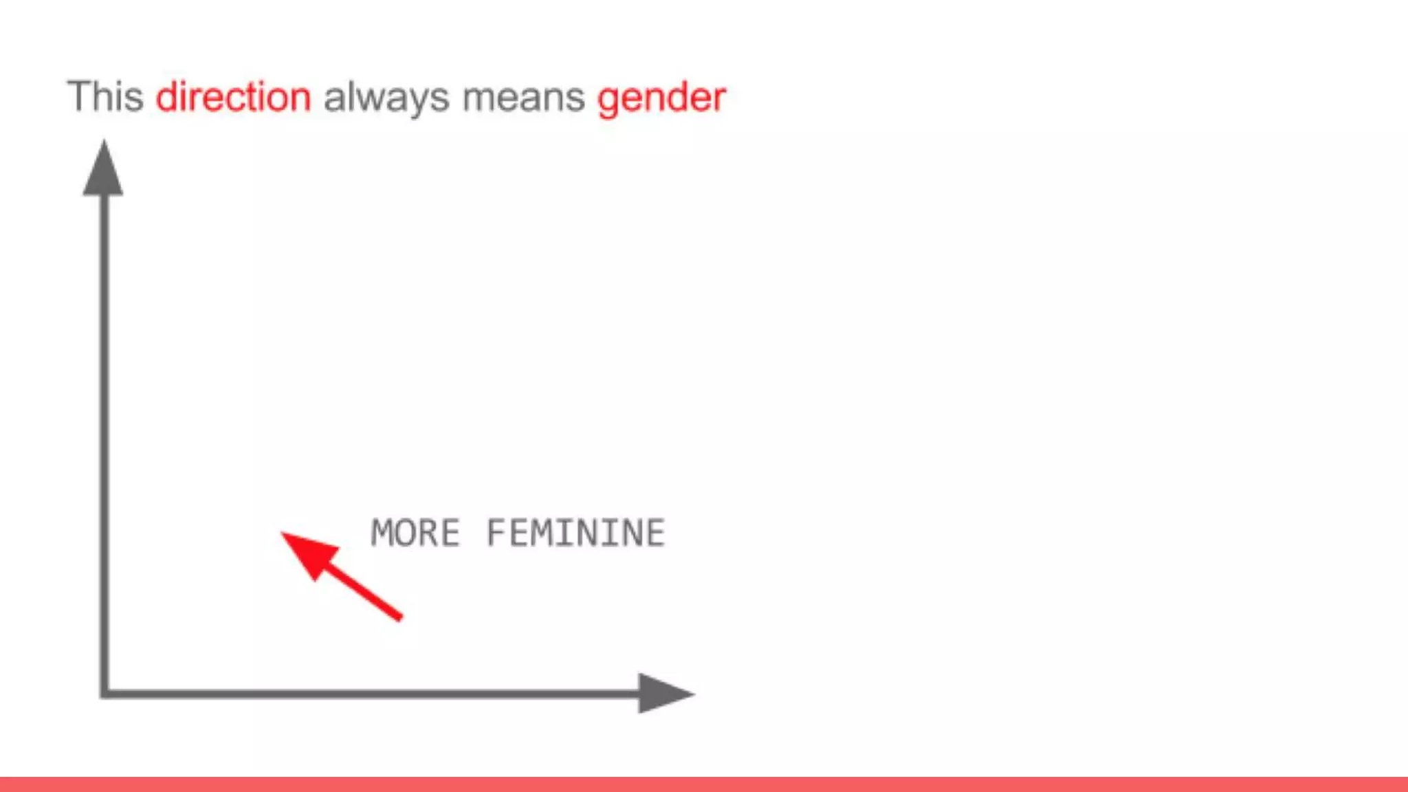
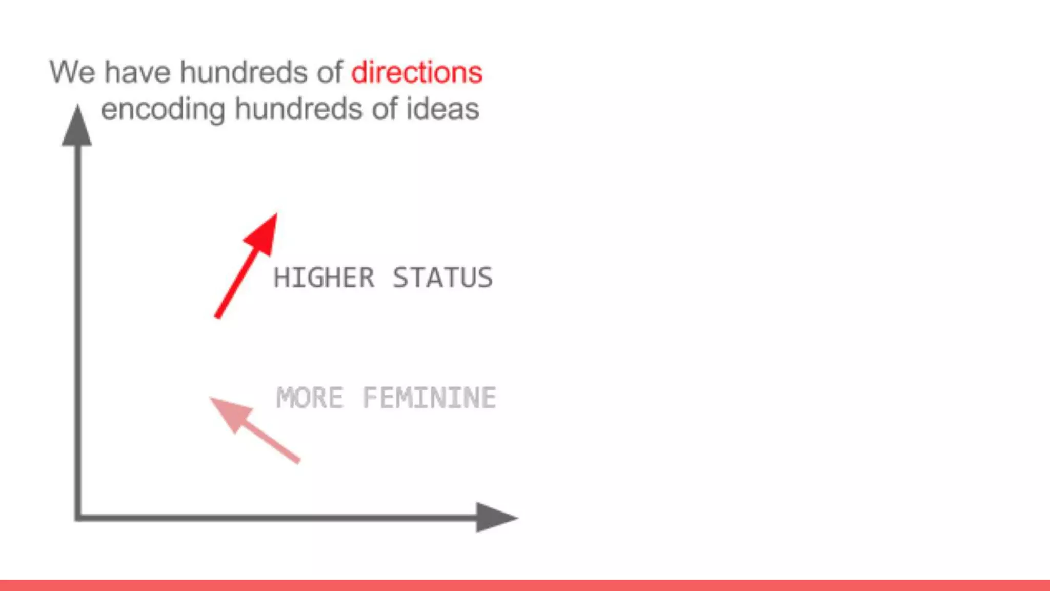
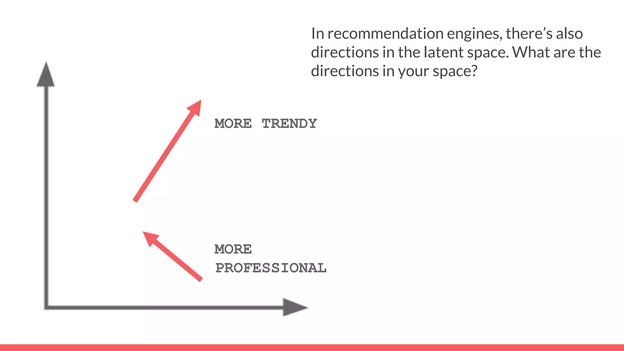
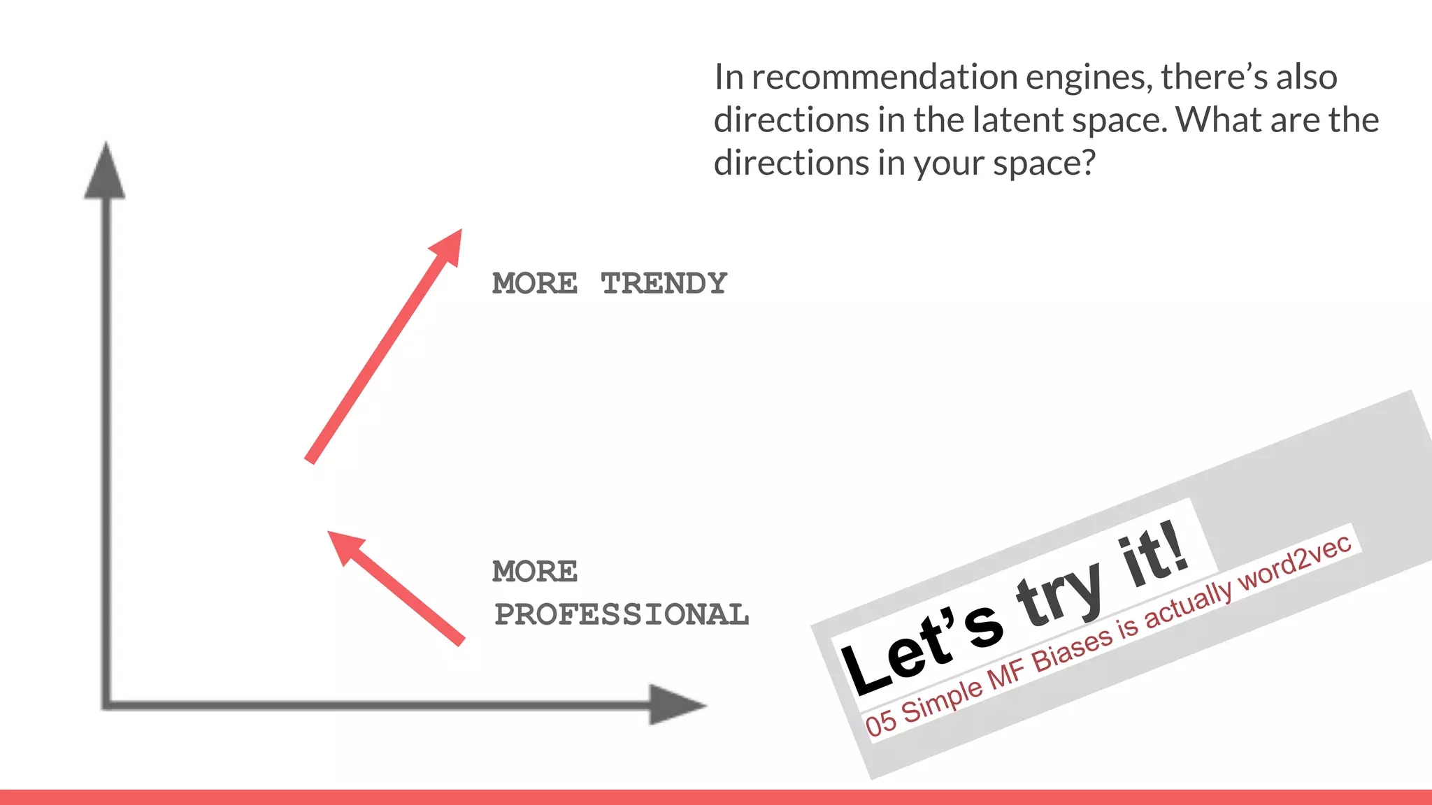
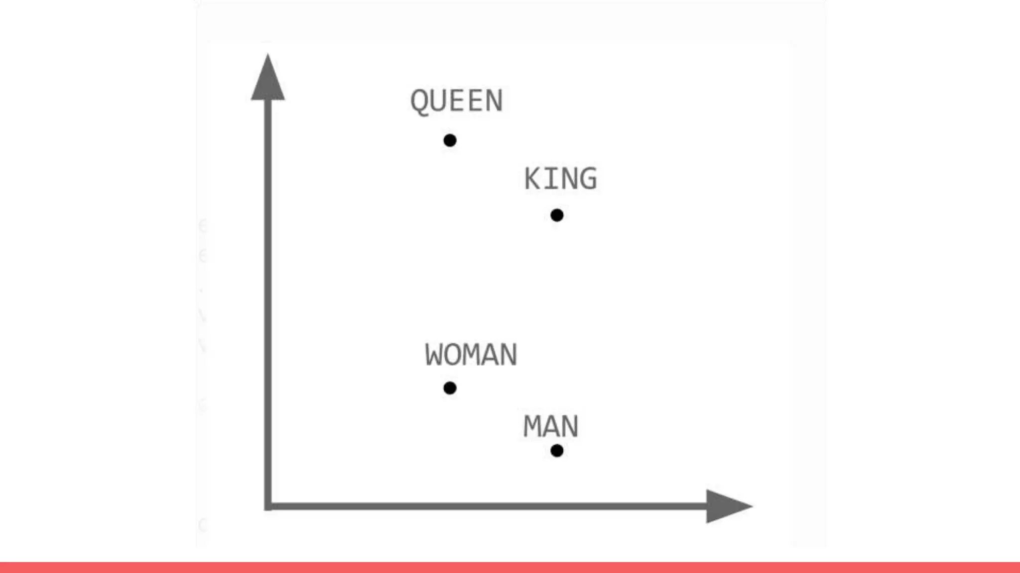
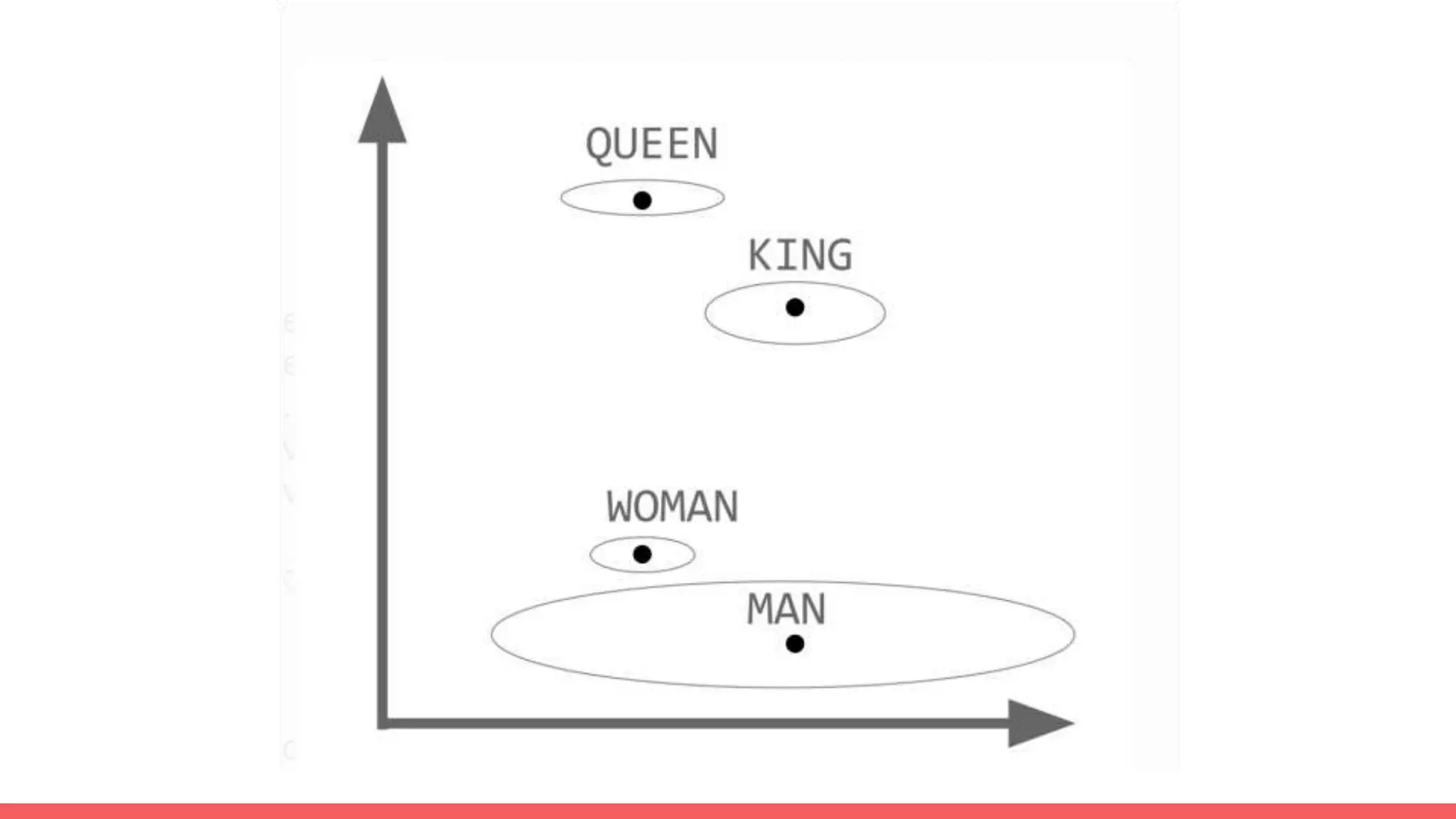
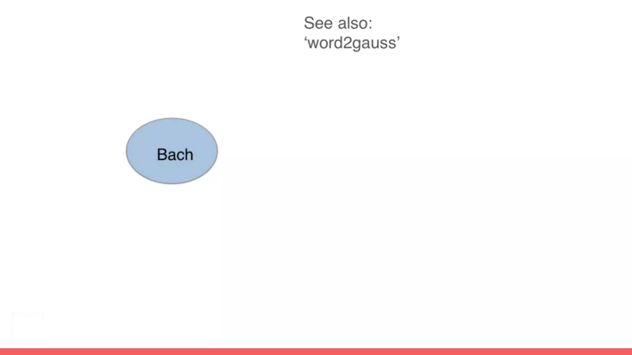
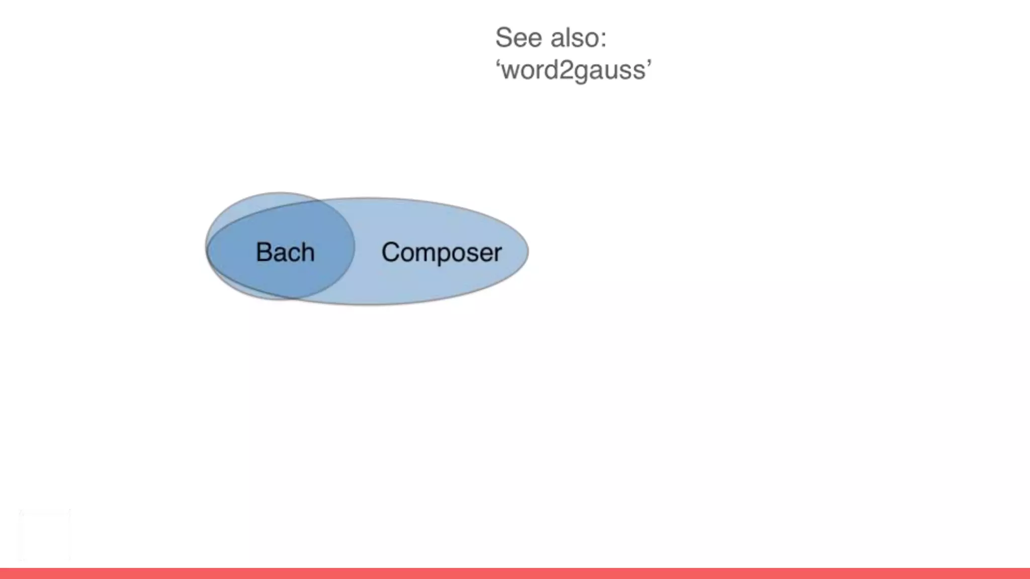
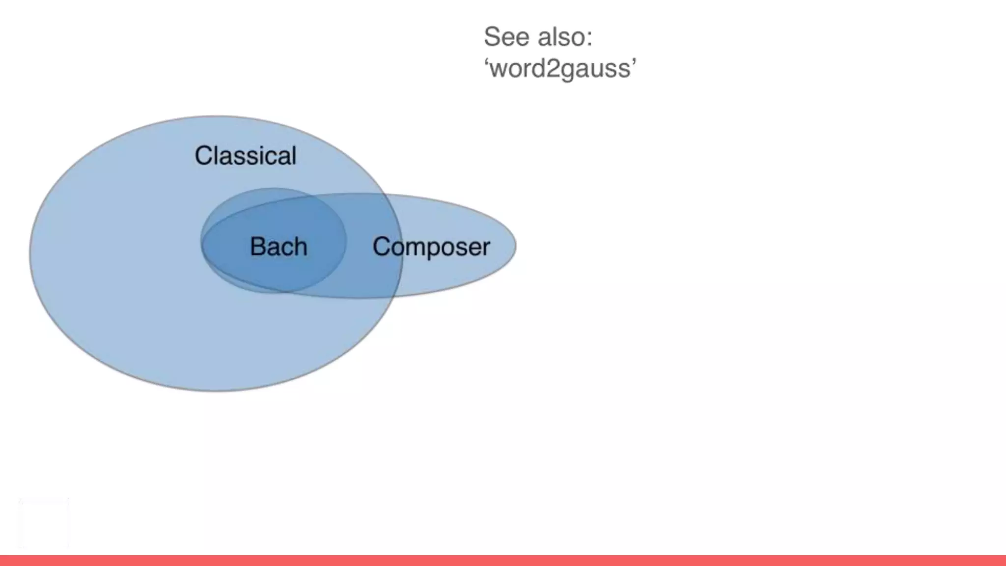
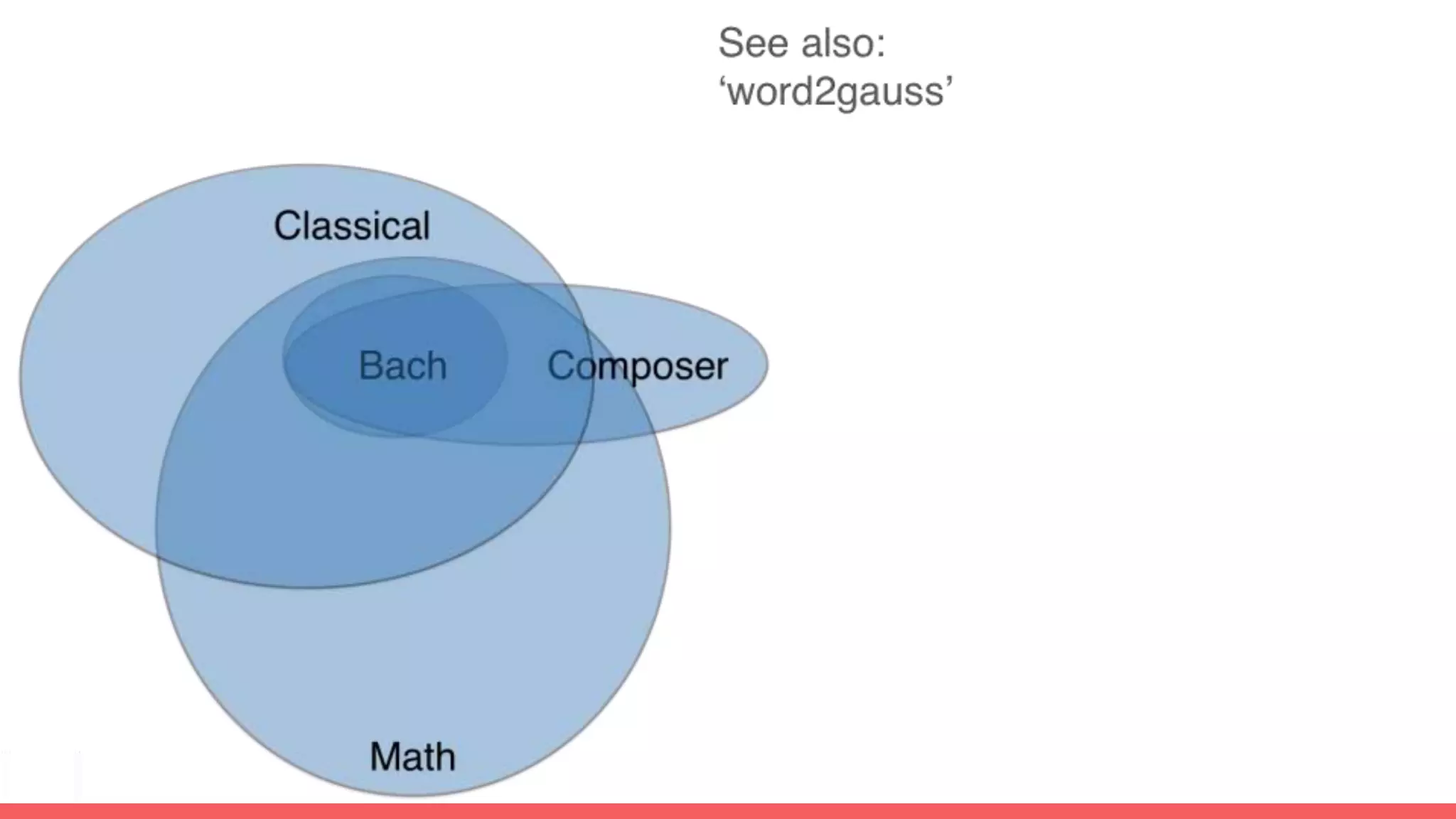
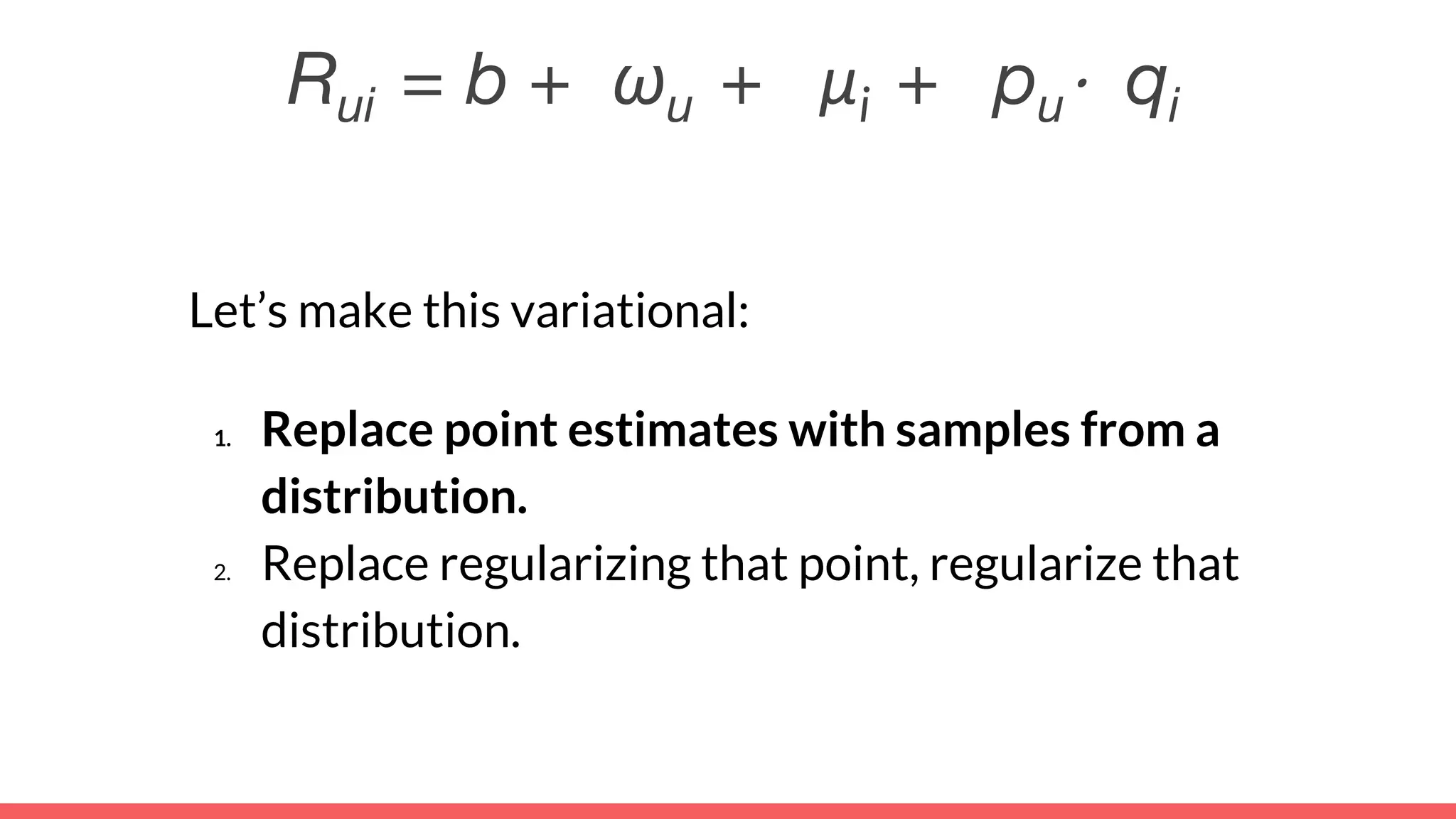
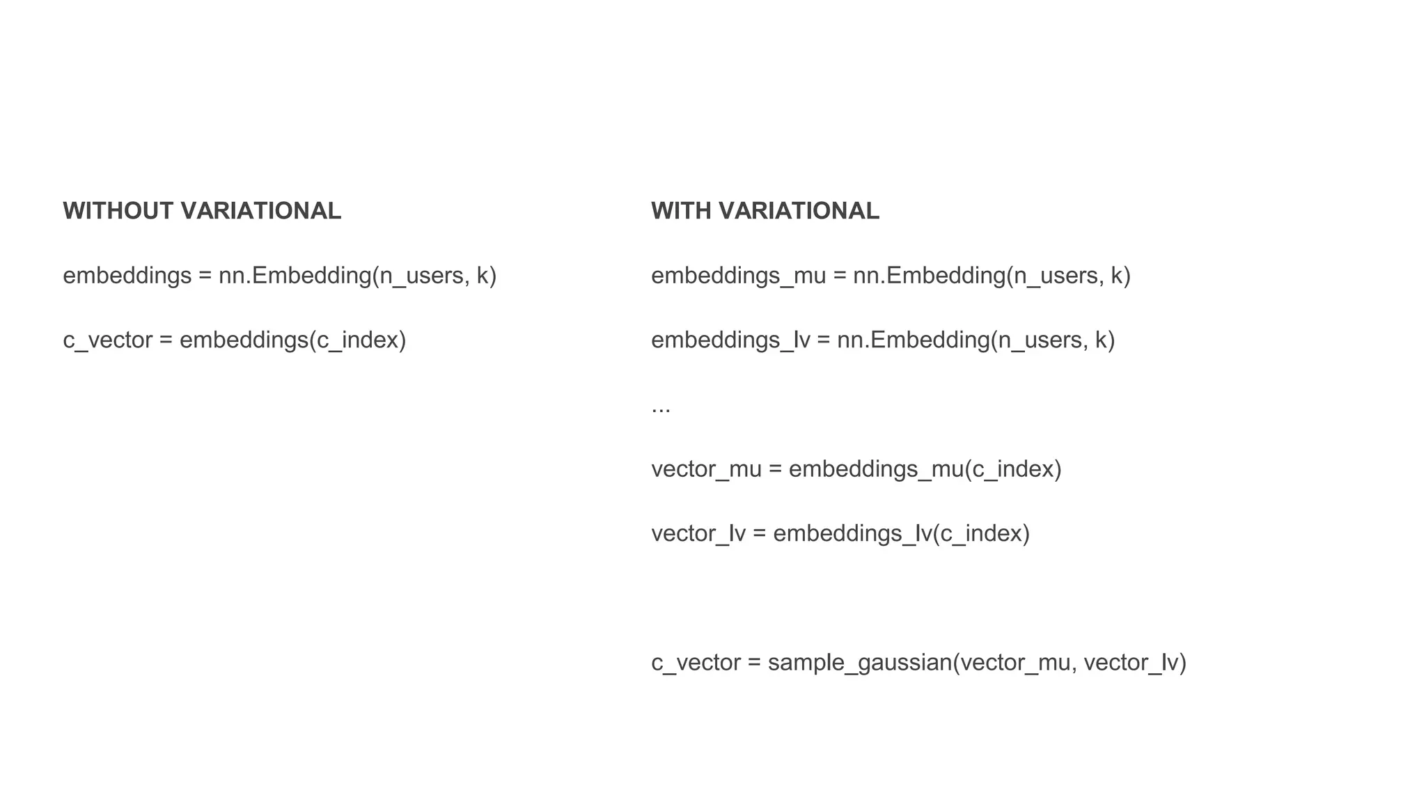
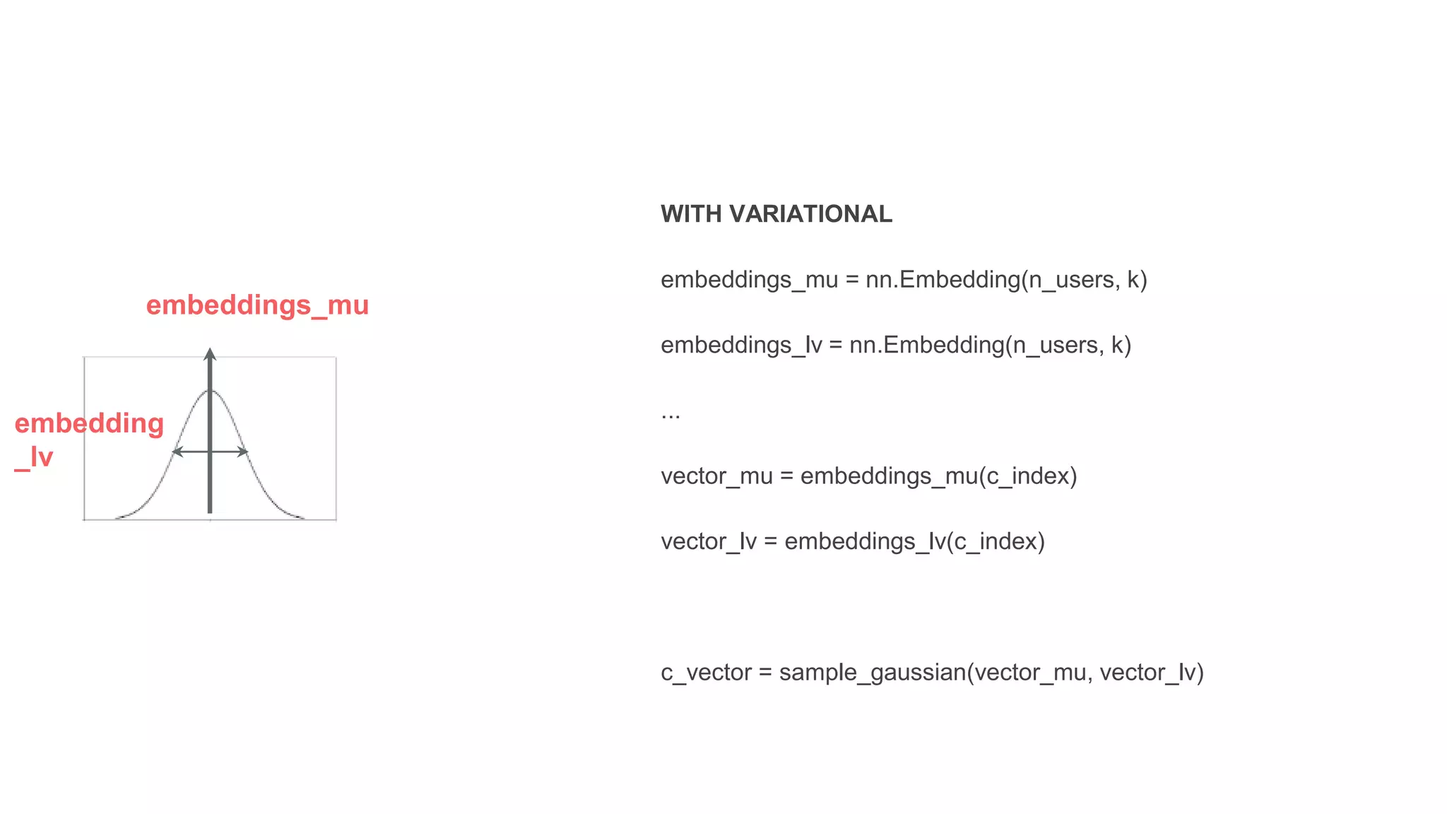
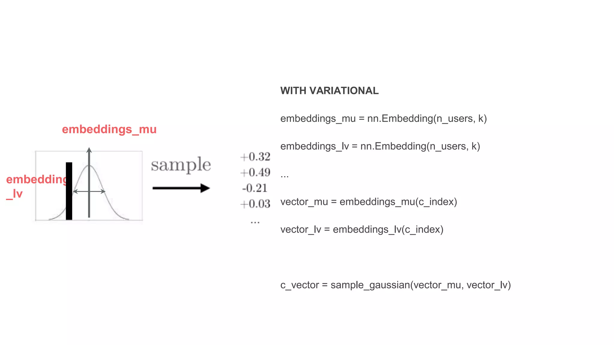
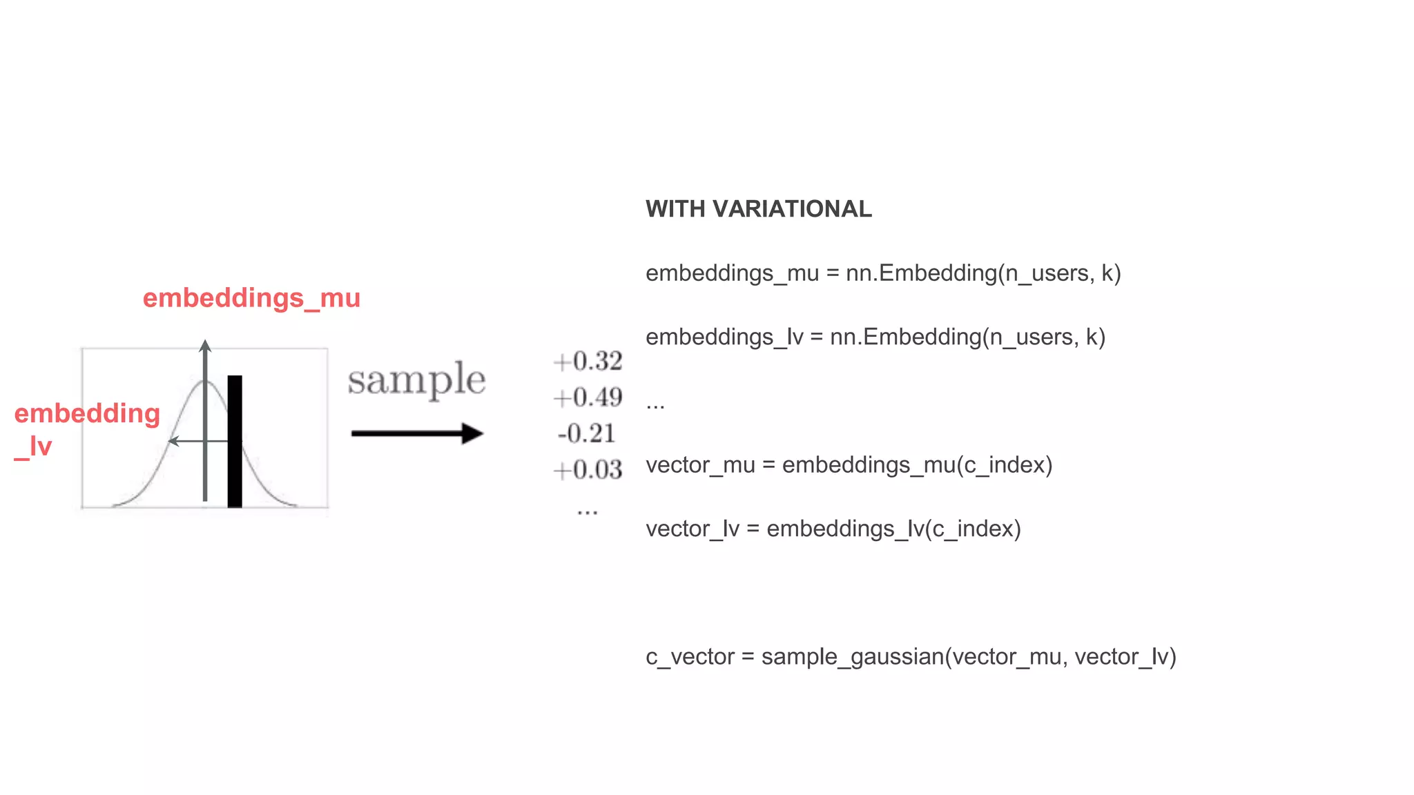
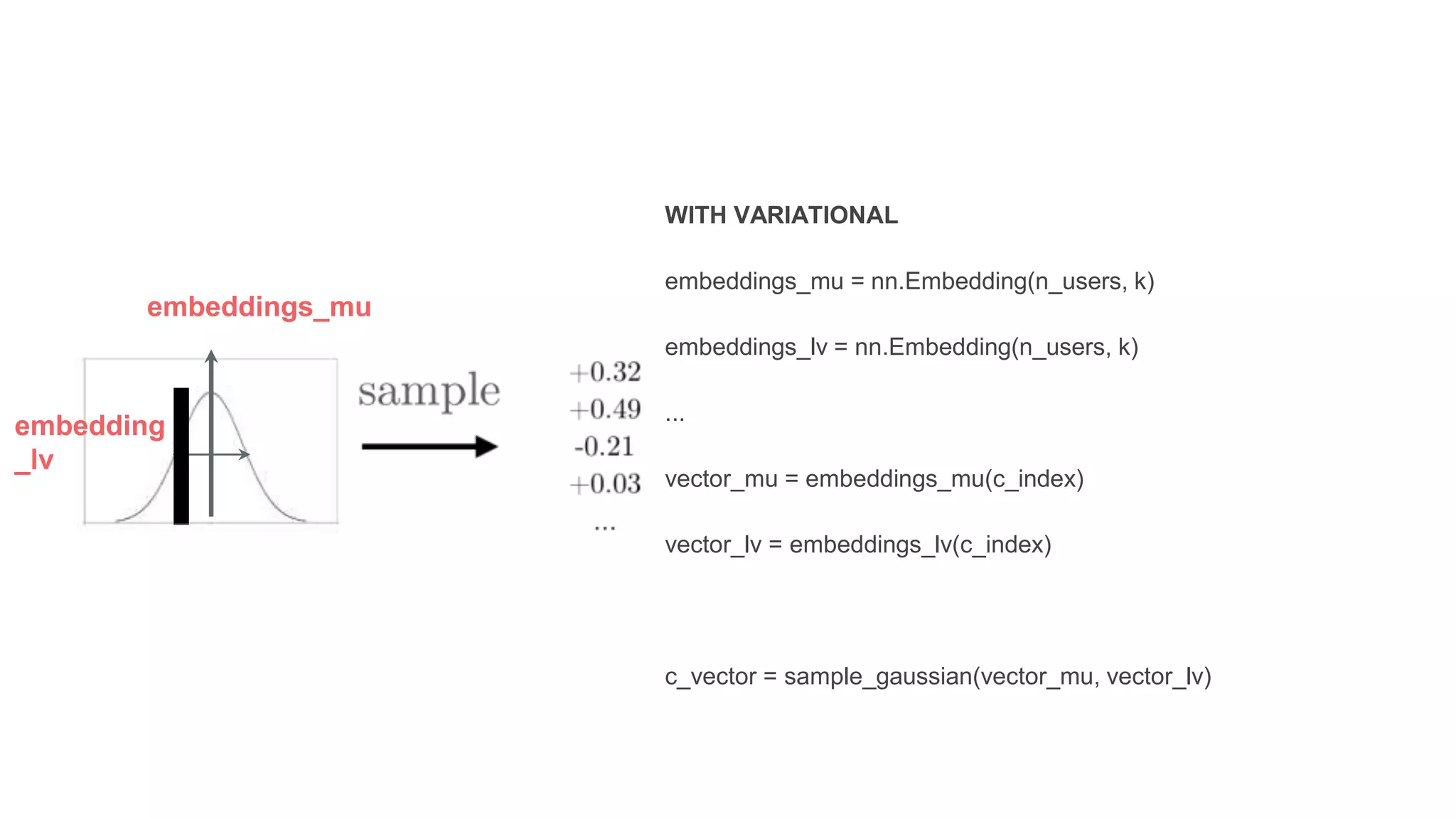
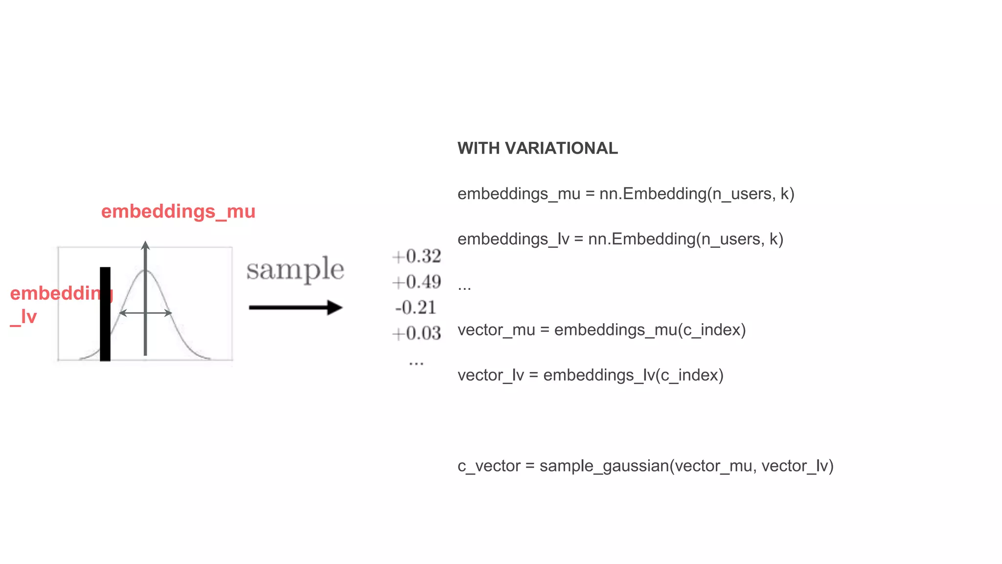
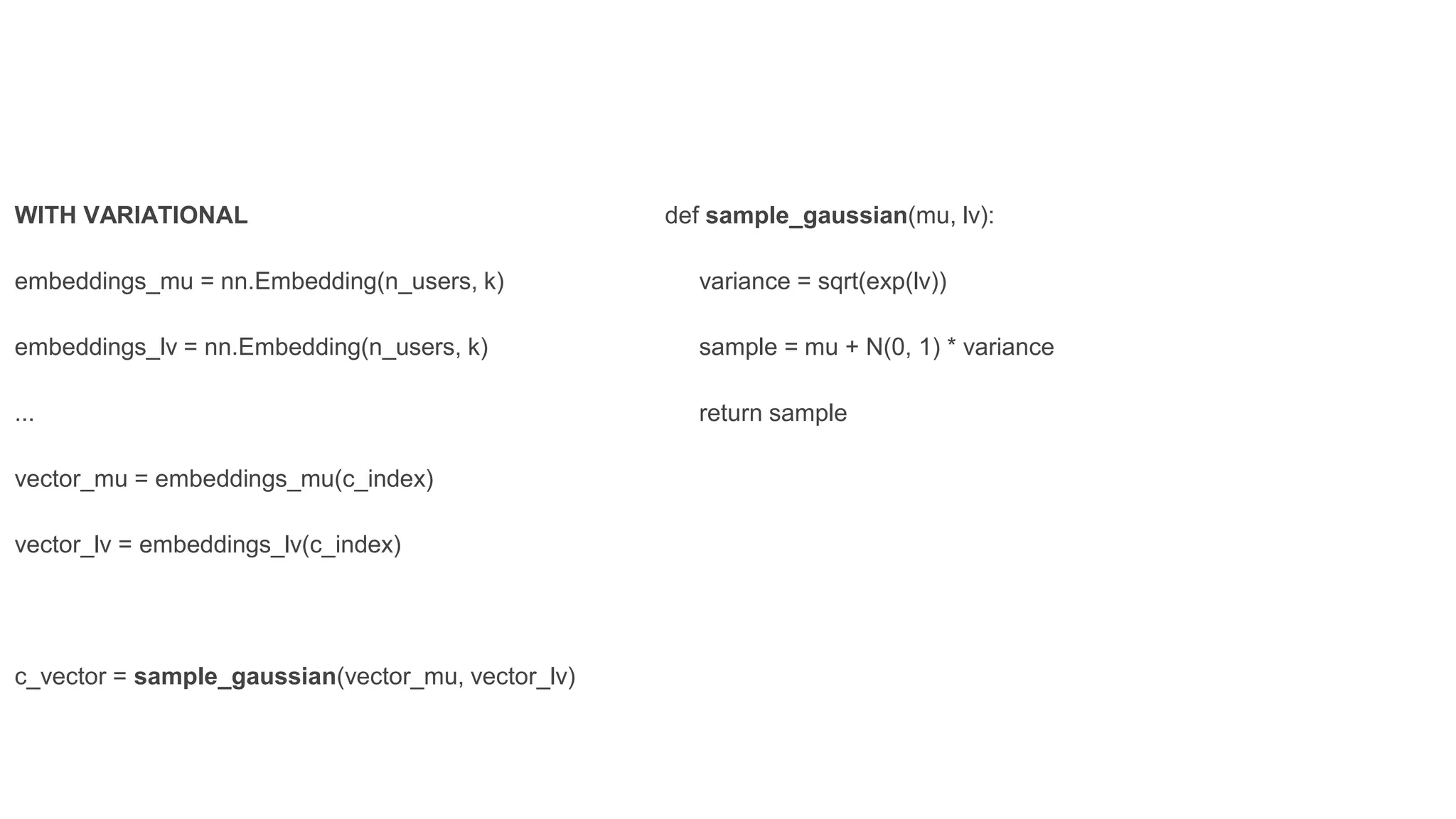
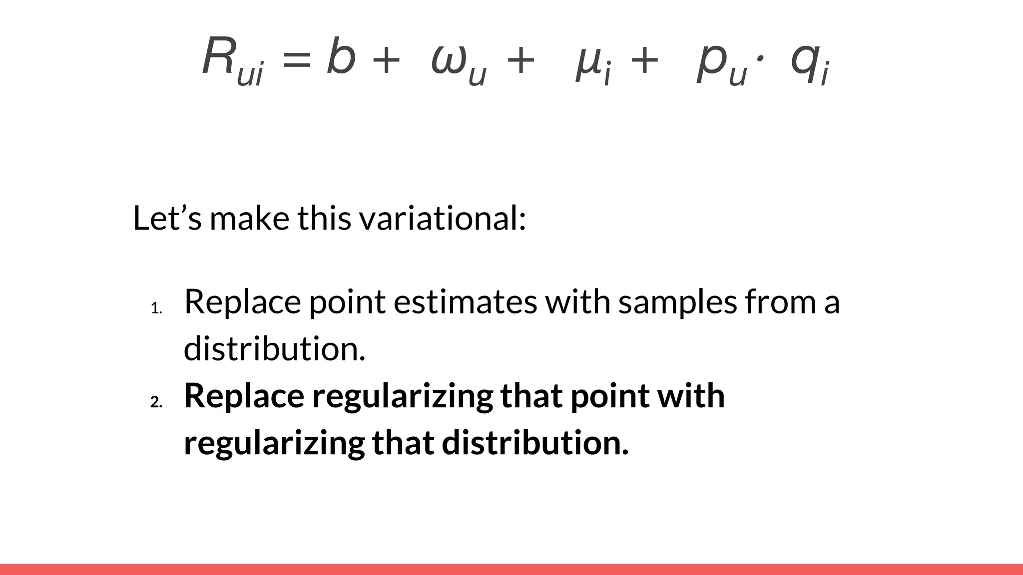
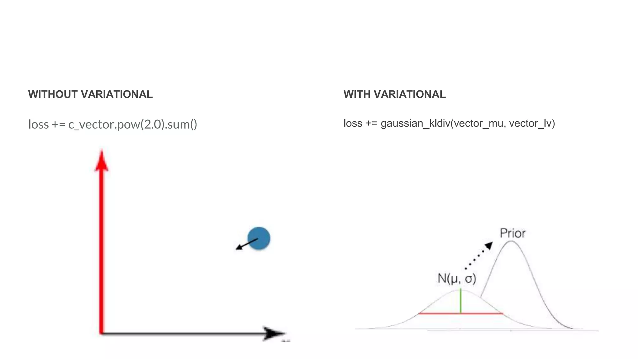
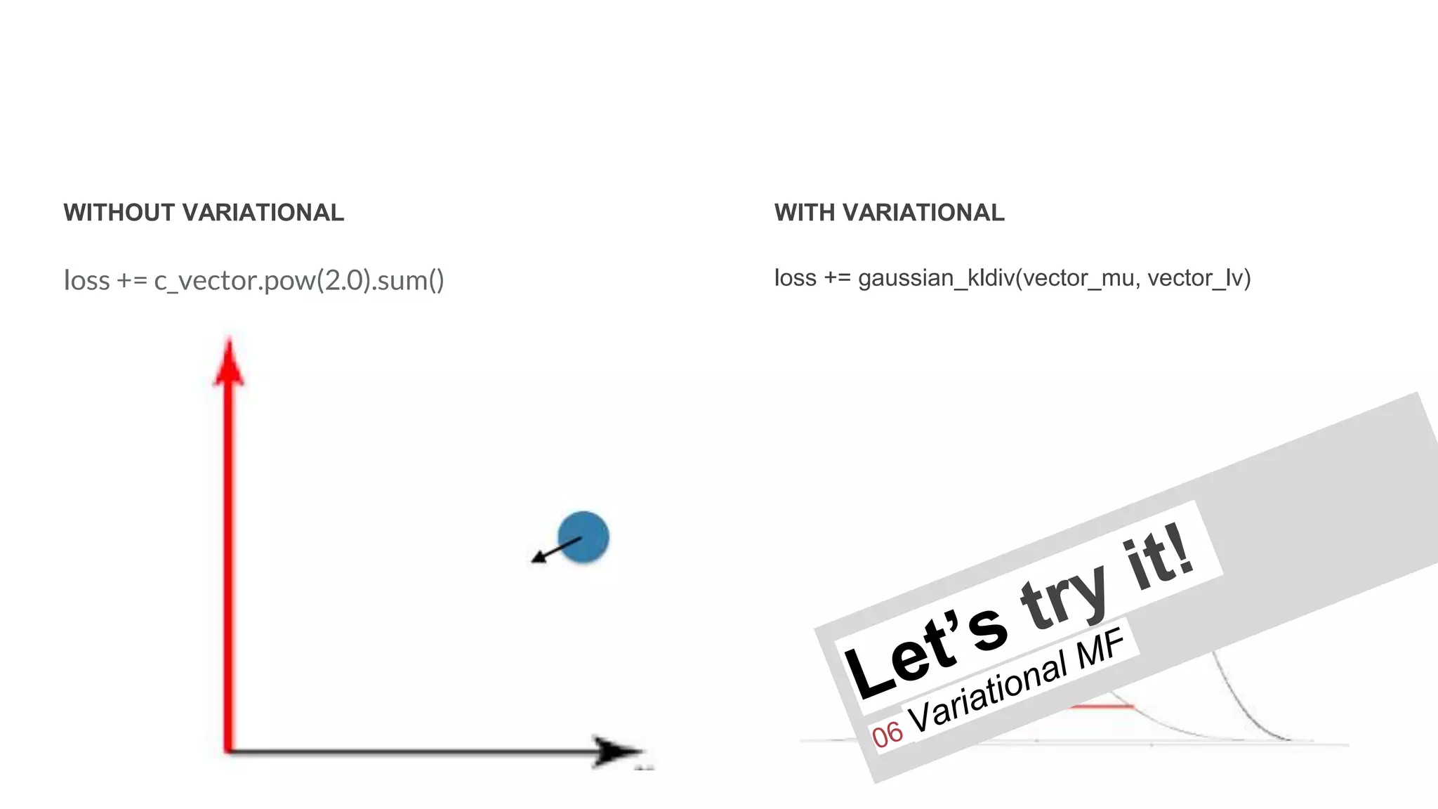
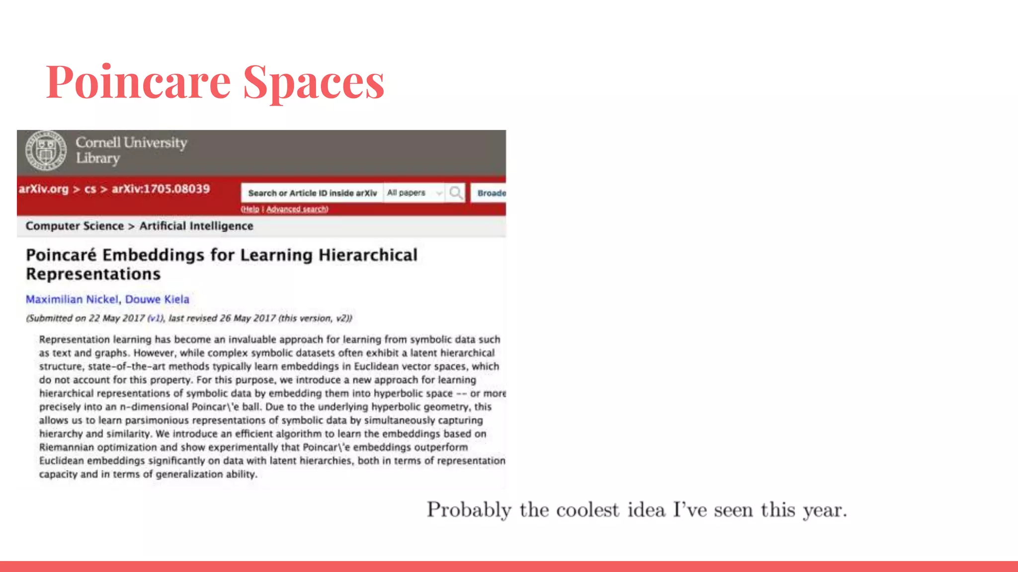
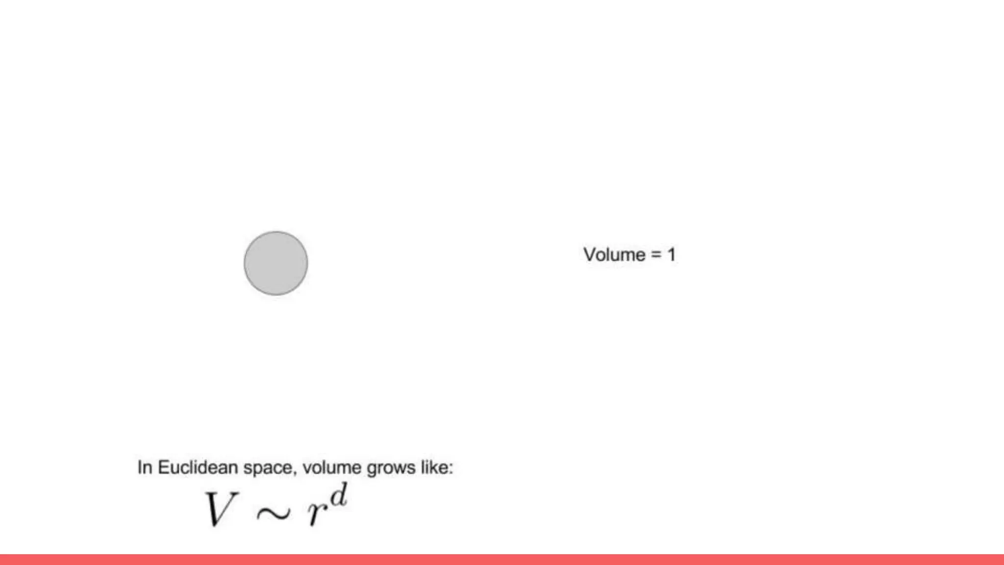
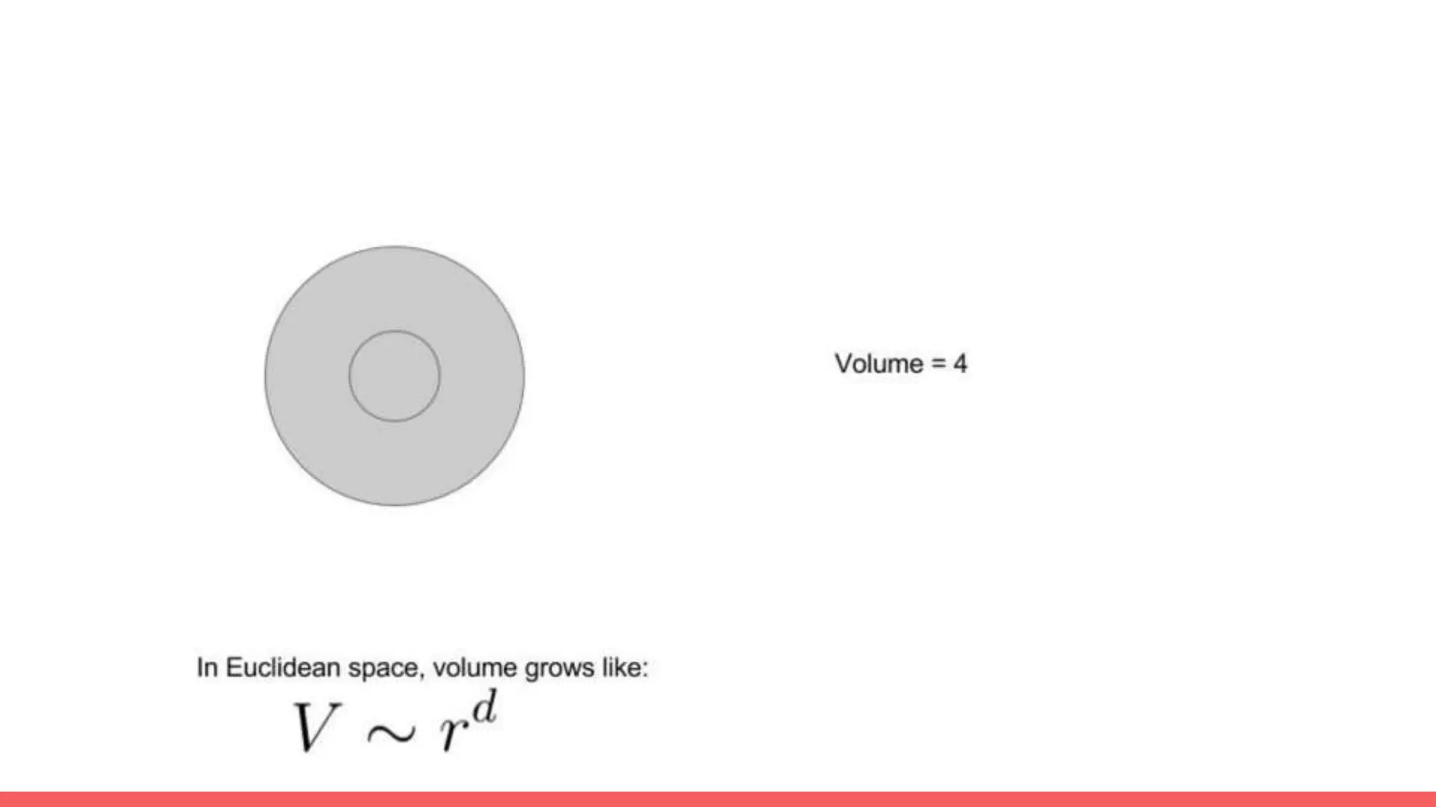
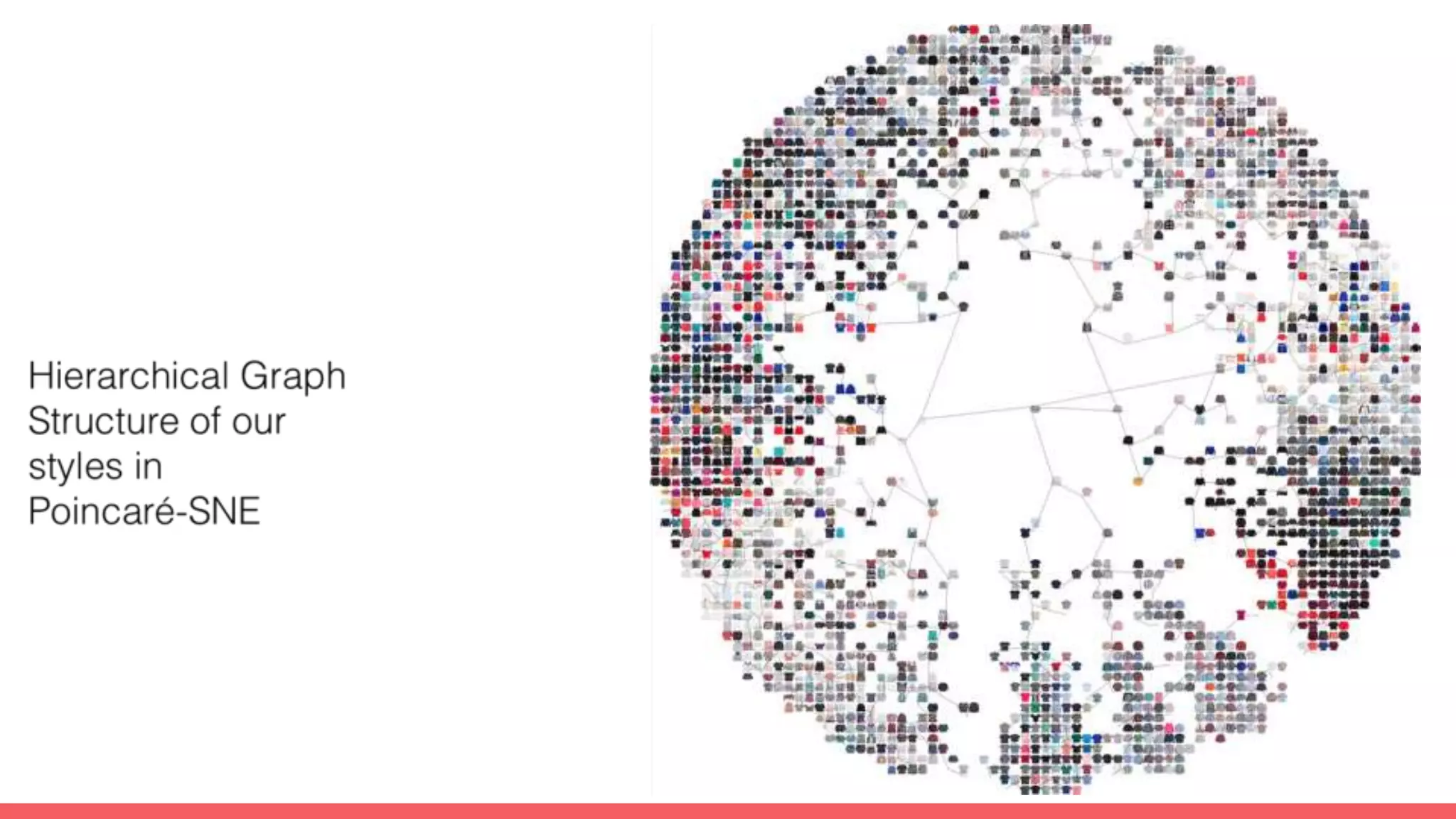
Deep
Recommendations
in PyTorch
Setup
Follow along with instructions here:
cemoody.github.io/simple_mf
About
@chrisemoody
Caltech Physics
PhD. in Astrophysics + Supercomputing
Scikit-Learn t-SNE Contributor
Stitch Fix AI Team
Stitch Fix
Stitch Fix
Stitch Fix
Stitch Fix
Stitch Fix
AI at Stitch Fix
Capture Joint
Annotation
Segmentation
Model Fitting
If you’re
interested, ask
me about this
later!
Matrix
Factorization
“Latent” Style Space
Matrix
Factorization
t-SNE Viz
“Latent” Style Space
100+ Data Scientists
Increased Personalization
Decreased Client Churn
Increased Personalization
Decreased Client Churn
Increased Item Sales
Increased Personalization
Decreased Client Churn
Increased Item Sales
Better Merch Buying
Increased Personalization
Decreased Client Churn
Increased Item Sales
Better Merch Buying
Better Stylist Relationships
1. More data means more personalization
1. Recommendation engines are instruments of your business.
1. Custom models respect your heterogeneous and unique system
Lessons Learned
Lessons Learned Goals for Today
1. More data means more personalization
We’ll use rec engines to drive personalization
1. Recommendation engines are instruments of your business.
The latent factors they reveal enable new science!
1. Custom models respect your heterogeneous and unique system
We’ll explore 8 different ways of building
deep recommendation engines.
Setup
Follow along with instructions here:
cemoody.github.io/simple_mf
Why PyTorch
This gets very deep.
…PyTorch
computes
everything at
run time… so
debug &
investigate!
…PyTorch
computes
everything at
run time… so
debug &
investigate!
Setup
Setup
Follow along with instructions here:
cemoody.github.io/simple_mf
Start Jupyter Notebook
Start Tensorboard
There are eight Jupyter
Notebooks in this tutorial.
We’ll go through them one-by-
one.
Feel free to run them in advance
-- they’ll start training models in
the background.
… or start them up as I go along.
Matrix Factorization
Fundamentals
Notebooks we’ll be using:
01 Training a simple MF model.ipynb
02 Simple MF Model with Biases.ipynb
+1
-1
+1
+1
0
+1
0
+1
+1+1
+1
0
+1
0
+1
+1
0
+1
0
+1
0
+1
0
+1
0
+1
0
+1 R
(n_users x n_items)
R
The ratings matrix
(n_users x n_items)
Extremely large
(Easily tens of billions of elements)
Mostly zeroes
(Typical sparsity is 0.01% - 1%)
R
The ratings matrix
(n_users, n_items)
P
The user matrix
(n_users, k)
Q
The item matrix
(n_item, k)
P
The user matrix
(n_users, k)
Q
The item matrix
(n_item, k)
Much smaller!
(millions or 100ks of rows)
Compact & dense!
No zeroes, efficient storage.
Rui ≈ pu⋅ qi
≈u
i
u
i
Rui ≈ pu⋅ qi
≈
A single +1 or 0 rating User vector
Item vector
known to be estimated
Minimize L = (Rui - pu⋅ qi)2
Minimize L = (Rui - pu⋅ qi)2 + c |Q|2 + c|P|2
Baseline model
- Only captures interactions.
- What if a user generally likes everything?
- What if an item is generally popular?
Rui = pu⋅ qi
Baseline model
- Only captures interactions.
- What if a user generally likes everything?
- What if an item is generally popular?
Let’s add biases.
Rui = pu⋅ qi
Model +
global bias
user biases
item biases
Now we learn how much a user
generally likes things, and an item is
generally liked.
Rui = b + ωu + μi + pu⋅ qi
A single +1 or 0 rating
User vector Item vectorUser bias
One number
per user
Item bias
One number
per item
=
Rui = b + ωu + μi + pu⋅ qi
A single +1 or 0 rating
User vector Item vectorUser bias
One number
per user
Rui = b + ωu + μi + pu⋅ qi
Item bias
One number
per item
=
Recommendation Engines
are an instrument to do science
User vector Item vector
User & item vectors are not black boxes.
They are instruments into your space.
Stitch Fix vectors stand for clothing style.
Movielens vectors yield movie genres.
At Spotify, they represent latent musical tastes.
Amazon they represent latent categories.
Let’s PCA the Stitch Fix vectors and take a look.
+1.2 - 0.3 +0.4 -4.0 +0.9
+6.7 - 0.44 + 0.9 +0.58 -0.7
+3.8 - 0.9 -2. 4 +0.8 +0.3
We’ll sort by the
first eigenvector.
+1.2 - 0.3 +0.4 -4.0 +0.9
+6.7 - 0.44 + 0.9 +0.58 -0.7
+3.8 - 0.9 -2. 4 +0.8 +0.3
Let’s PCA the Stitch Fix vectors and take a look.
Positive EndNegative End
striped,
polka dotted,
fitted,
button-up,
high chroma
this must be: preppy.
tile-printed,
paisley,
bell-sleeved,
fringed,
tasseled,
maxi
this must be: boho.
we did not define boho or preppy -- we discovered it!
This is the cornerstone of our ‘style space’ that segments our clients and
our merch.
+1.2 - 0.3 +0.4 -4.0 +0.9
+6.7 - 0.44 + 0.9 +0.58 -0.7
+3.8 - 0.9 -2. 4 +0.8 +0.3
We don’t have just one
dimension however….
… we have many more.
What do each of those
look like?
Internally, we use 18
dimensions.
The first three we call
trendiness, femininity,
and end use.
For more search:
“Understanding Latent
Style”
https://multithreaded.stitch
fix.com/blog/2018/06/28/la
tent-style/
Advanced Matrix
Factorization
Notebooks we’ll be using:
01 Training a simple MF model.ipynb
02 Simple MF Model with Biases.ipynb
This is now a typical matrix-
factorization recommender.
Rui = b + ωu + μi + pu⋅ qi
This is now a typical matrix-
factorization recommender.
What if we know more “side” features
-- like the user’s occupation?
Great for when we want to “coldstart”
a new user.
Rui = b + ωu + μi + pu⋅ qi
We have two choices for side features:
- add them as a bias
→ Choose this if you think occupation changes like rate, but not which
movies
→e.g. “artists like movies more than other occupations”
- add them as a user vector
→ Choose this if you think occupation changes depending on the item
→e.g. “realtors love real estate shows”
Rui = b + do + ωu + μi + ( pu+ to)⋅ qi
*Note that to interacts with qi
We have two choices for side features:
- add them as a bias
→ Choose this if you think occupation changes like rate, but not which
movies
→e.g. “realtors love real estate shows”
- add them as a user vector
→ Choose this if you think occupation changes movie selection
→e.g. “realtors love real estate shows”
Rui = b + do + ωu + μi + ( pu+ to)⋅ qi
*Note that to interacts with qi
Rui = b + ωu + μi + pu⋅ qi
What about when features change in time?
You’ve seen biases.
You’ve seen user-item interactions.
Rui = b + ωu + μi + pu⋅ qi + mu⋅ nt
What does a latent temporal vector encode?
Here’s a toy example.
t (time)
m0= 0.0 1.0
Average
User
Rating
0 1 2 3 4 5 6
0.0 1.0
Rui = b + ωu + μi + pu⋅ qi + mu⋅ nt
What does a latent temporal vector encode?
Here’s a toy example.
t (time)
m0= 0.0 1.0
Average
User
Rating
n0 = 1.0 0.0
n1 =
nt = 1 - t t0 1 2 3 4 5 6
0.9 0.1
0.0 1.0
Rui = b + ωu + μi + pu⋅ qi + mu⋅ nt
What does a latent temporal vector encode?
Here’s a toy example.
t (time)
Average
User
Rating
0 1 2 3 4 5 6
m1= 0.0 1.0
n0 = 1.0 0.0
n1 =
nt = 1 - t t
0.9 0.1
1.0 0.0
Rui = b + ωu + μi + pu⋅ qi + mu⋅ nt
What does a latent temporal vector encode?
A user mixture of time-series.
m1= 0.0 1.0
n0 = 1.0 0.0
n1 =
nt = 1 - t t
0.9 0.1
1.0 0.0
m0= 0.0 1.00.0 1.0
User 0 will have a
100% mixture of
the 1st time series
User 1 will have a
100% mixture of
the 2nd time series
Rui = b + ωu + μi + pu⋅ qi + mu⋅ nt
We can enforce that nearby times have
similar components.
n0 = 1.0 0.0
n1 =
nt = 1 - t t
0.9 0.1
Enforce that:
|nt - nt-1|
should be small.
Word2Vec is
actually a rec engine!
Notebooks we’ll be using:
03 Simple MF Biases is actually word2vec.ipynb
“ITEM_92 I think this fabric is wonderful
(rayon & spandex). like the lace/embroidery
accents”
Instead of
(users, items) we have (token1, token2)
And instead of a
Rating we have a skipgram count.
But it’s still the same model!
Rui = b + ωu + μi + pu⋅ qi
Item bias
token2 bias
User bias
token1 bias
A single +1 or 0 rating
Log Skipgram count
User vector
token1 vector
Item vector
token2 vector
=
Rui = ωu + μi + pu⋅ qi
User bias
token1 bias
(How frequent
is this word?)
A single +1 or 0 rating
Log Skipgram count
User vector
word1 vector
Item vector
word2 vector
Item bias
token2 bias
(How frequent is
this word?)
=
Rui = ωu + μi + pu⋅ qi
Do word1 & word2 have a
special interaction?
In recommendation engines, there’s also
directions in the latent space. What are the
directions in your space?
MORE TRENDY
MORE
PROFESSIONAL
In recommendation engines, there’s also
directions in the latent space. What are the
directions in your space?
MORE TRENDY
MORE
PROFESSIONAL
Variational Matrix
Factorization
Notebooks we’ll be using:
08 Variational MF.ipynb
Practical reasons to go variational:
1. Alternative regularization
2. Measure what your model doesn’t know.
3. Help explain your data.
Practical reasons to go variational:
1. Alternative regularization
2. Measure what your model doesn’t know.
3. Help explain your data.
4. Short & fits in a tweet!
Rui = b + ωu + μi + pu⋅ qi
Let’s make this variational:
1. Replace point estimates with samples from a
distribution.
2. Replace regularizing that point, regularize that
distribution.
WITHOUT VARIATIONAL
embeddings = nn.Embedding(n_users, k)
c_vector = embeddings(c_index)
WITH VARIATIONAL
embeddings_mu = nn.Embedding(n_users, k)
embeddings_lv = nn.Embedding(n_users, k)
...
vector_mu = embeddings_mu(c_index)
vector_lv = embeddings_lv(c_index)
c_vector = sample_gaussian(vector_mu, vector_lv)
WITH VARIATIONAL
embeddings_mu = nn.Embedding(n_users, k)
embeddings_lv = nn.Embedding(n_users, k)
...
vector_mu = embeddings_mu(c_index)
vector_lv = embeddings_lv(c_index)
c_vector = sample_gaussian(vector_mu, vector_lv)
embeddings_mu
embedding
_lv
WITH VARIATIONAL
embeddings_mu = nn.Embedding(n_users, k)
embeddings_lv = nn.Embedding(n_users, k)
...
vector_mu = embeddings_mu(c_index)
vector_lv = embeddings_lv(c_index)
c_vector = sample_gaussian(vector_mu, vector_lv)
embeddings_mu
embedding
_lv
WITH VARIATIONAL
embeddings_mu = nn.Embedding(n_users, k)
embeddings_lv = nn.Embedding(n_users, k)
...
vector_mu = embeddings_mu(c_index)
vector_lv = embeddings_lv(c_index)
c_vector = sample_gaussian(vector_mu, vector_lv)
embeddings_mu
embedding
_lv
WITH VARIATIONAL
embeddings_mu = nn.Embedding(n_users, k)
embeddings_lv = nn.Embedding(n_users, k)
...
vector_mu = embeddings_mu(c_index)
vector_lv = embeddings_lv(c_index)
c_vector = sample_gaussian(vector_mu, vector_lv)
embeddings_mu
embedding
_lv
WITH VARIATIONAL
embeddings_mu = nn.Embedding(n_users, k)
embeddings_lv = nn.Embedding(n_users, k)
...
vector_mu = embeddings_mu(c_index)
vector_lv = embeddings_lv(c_index)
c_vector = sample_gaussian(vector_mu, vector_lv)
embeddings_mu
embedding
_lv
def sample_gaussian(mu, lv):
variance = sqrt(exp(lv))
sample = mu + N(0, 1) * variance
return sample
WITH VARIATIONAL
embeddings_mu = nn.Embedding(n_users, k)
embeddings_lv = nn.Embedding(n_users, k)
...
vector_mu = embeddings_mu(c_index)
vector_lv = embeddings_lv(c_index)
c_vector = sample_gaussian(vector_mu, vector_lv)
Rui = b + ωu + μi + pu⋅ qi
Let’s make this variational:
1. Replace point estimates with samples from a
distribution.
2. Replace regularizing that point with
regularizing that distribution.
WITH VARIATIONAL
loss += gaussian_kldiv(vector_mu, vector_lv)
WITHOUT VARIATIONAL
loss += c_vector.pow(2.0).sum()
WITH VARIATIONAL
loss += gaussian_kldiv(vector_mu, vector_lv)
WITHOUT VARIATIONAL
loss += c_vector.pow(2.0).sum()
At the Frontier
More Things to Try
FMs
● Useful when you have many kinds of
interactions, not just user-item and user-
time
Mixture-of-Tastes
● Like “attention” for recommendations,
allows for users to have multiple “tastes.”
Extra: Non-Euclidean Spaces
Poincare Spaces
“Zelda” is a game in set 2D Euclidean space
(roughly).
● Infinity can’t be seen
● Area is homogenous
● Geodesics are straight lines
“Hyper Rogue” is a game in hyperbolic
space.
● Radius = 1 is infinitely far away,
but visible
● Volume increases towards
boundary
“Hyper Rogue” is a game in hyperbolic
space.
● Radius = 1 is infinitely far away,
but visible
● Volume increases towards
boundary
Deep recommendations in PyTorch

Deep recommendations in PyTorch

  • 1.
  • 2.
    Setup Follow along withinstructions here: cemoody.github.io/simple_mf
  • 3.
    About @chrisemoody Caltech Physics PhD. inAstrophysics + Supercomputing Scikit-Learn t-SNE Contributor Stitch Fix AI Team
  • 4.
  • 5.
  • 6.
  • 7.
  • 8.
  • 9.
    AI at StitchFix Capture Joint Annotation Segmentation Model Fitting If you’re interested, ask me about this later!
  • 10.
  • 11.
  • 12.
  • 13.
  • 14.
  • 15.
  • 16.
    Increased Personalization Decreased ClientChurn Increased Item Sales Better Merch Buying
  • 17.
    Increased Personalization Decreased ClientChurn Increased Item Sales Better Merch Buying Better Stylist Relationships
  • 18.
    1. More datameans more personalization 1. Recommendation engines are instruments of your business. 1. Custom models respect your heterogeneous and unique system Lessons Learned
  • 19.
    Lessons Learned Goalsfor Today 1. More data means more personalization We’ll use rec engines to drive personalization 1. Recommendation engines are instruments of your business. The latent factors they reveal enable new science! 1. Custom models respect your heterogeneous and unique system We’ll explore 8 different ways of building deep recommendation engines.
  • 20.
    Setup Follow along withinstructions here: cemoody.github.io/simple_mf
  • 21.
  • 28.
  • 30.
  • 31.
  • 32.
  • 33.
    Setup Follow along withinstructions here: cemoody.github.io/simple_mf
  • 34.
  • 35.
  • 36.
    There are eightJupyter Notebooks in this tutorial. We’ll go through them one-by- one. Feel free to run them in advance -- they’ll start training models in the background. … or start them up as I go along.
  • 37.
    Matrix Factorization Fundamentals Notebooks we’llbe using: 01 Training a simple MF model.ipynb 02 Simple MF Model with Biases.ipynb
  • 40.
  • 41.
  • 42.
  • 43.
  • 44.
  • 45.
    R The ratings matrix (n_usersx n_items) Extremely large (Easily tens of billions of elements) Mostly zeroes (Typical sparsity is 0.01% - 1%)
  • 46.
    R The ratings matrix (n_users,n_items) P The user matrix (n_users, k) Q The item matrix (n_item, k)
  • 47.
    P The user matrix (n_users,k) Q The item matrix (n_item, k) Much smaller! (millions or 100ks of rows) Compact & dense! No zeroes, efficient storage.
  • 48.
    Rui ≈ pu⋅qi ≈u i u i
  • 49.
    Rui ≈ pu⋅qi ≈ A single +1 or 0 rating User vector Item vector known to be estimated
  • 50.
    Minimize L =(Rui - pu⋅ qi)2
  • 51.
    Minimize L =(Rui - pu⋅ qi)2 + c |Q|2 + c|P|2
  • 52.
    Minimize L =(Rui - pu⋅ qi)2 + c |Q|2 + c|P|2
  • 53.
    Baseline model - Onlycaptures interactions. - What if a user generally likes everything? - What if an item is generally popular? Rui = pu⋅ qi
  • 54.
    Baseline model - Onlycaptures interactions. - What if a user generally likes everything? - What if an item is generally popular? Let’s add biases. Rui = pu⋅ qi
  • 55.
    Model + global bias userbiases item biases Now we learn how much a user generally likes things, and an item is generally liked. Rui = b + ωu + μi + pu⋅ qi
  • 56.
    A single +1or 0 rating User vector Item vectorUser bias One number per user Item bias One number per item = Rui = b + ωu + μi + pu⋅ qi
  • 57.
    A single +1or 0 rating User vector Item vectorUser bias One number per user Rui = b + ωu + μi + pu⋅ qi Item bias One number per item =
  • 58.
    Recommendation Engines are aninstrument to do science
  • 59.
    User vector Itemvector User & item vectors are not black boxes. They are instruments into your space. Stitch Fix vectors stand for clothing style. Movielens vectors yield movie genres. At Spotify, they represent latent musical tastes. Amazon they represent latent categories.
  • 60.
    Let’s PCA theStitch Fix vectors and take a look. +1.2 - 0.3 +0.4 -4.0 +0.9 +6.7 - 0.44 + 0.9 +0.58 -0.7 +3.8 - 0.9 -2. 4 +0.8 +0.3
  • 61.
    We’ll sort bythe first eigenvector. +1.2 - 0.3 +0.4 -4.0 +0.9 +6.7 - 0.44 + 0.9 +0.58 -0.7 +3.8 - 0.9 -2. 4 +0.8 +0.3 Let’s PCA the Stitch Fix vectors and take a look.
  • 62.
  • 63.
    striped, polka dotted, fitted, button-up, high chroma thismust be: preppy. tile-printed, paisley, bell-sleeved, fringed, tasseled, maxi this must be: boho.
  • 64.
    we did notdefine boho or preppy -- we discovered it! This is the cornerstone of our ‘style space’ that segments our clients and our merch.
  • 65.
    +1.2 - 0.3+0.4 -4.0 +0.9 +6.7 - 0.44 + 0.9 +0.58 -0.7 +3.8 - 0.9 -2. 4 +0.8 +0.3 We don’t have just one dimension however…. … we have many more. What do each of those look like?
  • 66.
    Internally, we use18 dimensions. The first three we call trendiness, femininity, and end use.
  • 67.
    For more search: “UnderstandingLatent Style” https://multithreaded.stitch fix.com/blog/2018/06/28/la tent-style/
  • 68.
    Advanced Matrix Factorization Notebooks we’llbe using: 01 Training a simple MF model.ipynb 02 Simple MF Model with Biases.ipynb
  • 69.
    This is nowa typical matrix- factorization recommender. Rui = b + ωu + μi + pu⋅ qi
  • 70.
    This is nowa typical matrix- factorization recommender. What if we know more “side” features -- like the user’s occupation? Great for when we want to “coldstart” a new user. Rui = b + ωu + μi + pu⋅ qi
  • 71.
    We have twochoices for side features: - add them as a bias → Choose this if you think occupation changes like rate, but not which movies →e.g. “artists like movies more than other occupations” - add them as a user vector → Choose this if you think occupation changes depending on the item →e.g. “realtors love real estate shows” Rui = b + do + ωu + μi + ( pu+ to)⋅ qi *Note that to interacts with qi
  • 72.
    We have twochoices for side features: - add them as a bias → Choose this if you think occupation changes like rate, but not which movies →e.g. “realtors love real estate shows” - add them as a user vector → Choose this if you think occupation changes movie selection →e.g. “realtors love real estate shows” Rui = b + do + ωu + μi + ( pu+ to)⋅ qi *Note that to interacts with qi
  • 73.
    Rui = b+ ωu + μi + pu⋅ qi What about when features change in time? You’ve seen biases. You’ve seen user-item interactions.
  • 74.
    Rui = b+ ωu + μi + pu⋅ qi + mu⋅ nt What does a latent temporal vector encode? Here’s a toy example. t (time) m0= 0.0 1.0 Average User Rating 0 1 2 3 4 5 6 0.0 1.0
  • 75.
    Rui = b+ ωu + μi + pu⋅ qi + mu⋅ nt What does a latent temporal vector encode? Here’s a toy example. t (time) m0= 0.0 1.0 Average User Rating n0 = 1.0 0.0 n1 = nt = 1 - t t0 1 2 3 4 5 6 0.9 0.1 0.0 1.0
  • 76.
    Rui = b+ ωu + μi + pu⋅ qi + mu⋅ nt What does a latent temporal vector encode? Here’s a toy example. t (time) Average User Rating 0 1 2 3 4 5 6 m1= 0.0 1.0 n0 = 1.0 0.0 n1 = nt = 1 - t t 0.9 0.1 1.0 0.0
  • 77.
    Rui = b+ ωu + μi + pu⋅ qi + mu⋅ nt What does a latent temporal vector encode? A user mixture of time-series. m1= 0.0 1.0 n0 = 1.0 0.0 n1 = nt = 1 - t t 0.9 0.1 1.0 0.0 m0= 0.0 1.00.0 1.0 User 0 will have a 100% mixture of the 1st time series User 1 will have a 100% mixture of the 2nd time series
  • 78.
    Rui = b+ ωu + μi + pu⋅ qi + mu⋅ nt We can enforce that nearby times have similar components. n0 = 1.0 0.0 n1 = nt = 1 - t t 0.9 0.1 Enforce that: |nt - nt-1| should be small.
  • 79.
    Word2Vec is actually arec engine! Notebooks we’ll be using: 03 Simple MF Biases is actually word2vec.ipynb
  • 80.
    “ITEM_92 I thinkthis fabric is wonderful (rayon & spandex). like the lace/embroidery accents”
  • 95.
    Instead of (users, items)we have (token1, token2) And instead of a Rating we have a skipgram count. But it’s still the same model! Rui = b + ωu + μi + pu⋅ qi
  • 96.
    Item bias token2 bias Userbias token1 bias A single +1 or 0 rating Log Skipgram count User vector token1 vector Item vector token2 vector = Rui = ωu + μi + pu⋅ qi
  • 97.
    User bias token1 bias (Howfrequent is this word?) A single +1 or 0 rating Log Skipgram count User vector word1 vector Item vector word2 vector Item bias token2 bias (How frequent is this word?) = Rui = ωu + μi + pu⋅ qi Do word1 & word2 have a special interaction?
  • 102.
    In recommendation engines,there’s also directions in the latent space. What are the directions in your space? MORE TRENDY MORE PROFESSIONAL
  • 103.
    In recommendation engines,there’s also directions in the latent space. What are the directions in your space? MORE TRENDY MORE PROFESSIONAL
  • 104.
    Variational Matrix Factorization Notebooks we’llbe using: 08 Variational MF.ipynb
  • 105.
    Practical reasons togo variational: 1. Alternative regularization 2. Measure what your model doesn’t know. 3. Help explain your data.
  • 106.
    Practical reasons togo variational: 1. Alternative regularization 2. Measure what your model doesn’t know. 3. Help explain your data. 4. Short & fits in a tweet!
  • 114.
    Rui = b+ ωu + μi + pu⋅ qi Let’s make this variational: 1. Replace point estimates with samples from a distribution. 2. Replace regularizing that point, regularize that distribution.
  • 115.
    WITHOUT VARIATIONAL embeddings =nn.Embedding(n_users, k) c_vector = embeddings(c_index) WITH VARIATIONAL embeddings_mu = nn.Embedding(n_users, k) embeddings_lv = nn.Embedding(n_users, k) ... vector_mu = embeddings_mu(c_index) vector_lv = embeddings_lv(c_index) c_vector = sample_gaussian(vector_mu, vector_lv)
  • 116.
    WITH VARIATIONAL embeddings_mu =nn.Embedding(n_users, k) embeddings_lv = nn.Embedding(n_users, k) ... vector_mu = embeddings_mu(c_index) vector_lv = embeddings_lv(c_index) c_vector = sample_gaussian(vector_mu, vector_lv) embeddings_mu embedding _lv
  • 117.
    WITH VARIATIONAL embeddings_mu =nn.Embedding(n_users, k) embeddings_lv = nn.Embedding(n_users, k) ... vector_mu = embeddings_mu(c_index) vector_lv = embeddings_lv(c_index) c_vector = sample_gaussian(vector_mu, vector_lv) embeddings_mu embedding _lv
  • 118.
    WITH VARIATIONAL embeddings_mu =nn.Embedding(n_users, k) embeddings_lv = nn.Embedding(n_users, k) ... vector_mu = embeddings_mu(c_index) vector_lv = embeddings_lv(c_index) c_vector = sample_gaussian(vector_mu, vector_lv) embeddings_mu embedding _lv
  • 119.
    WITH VARIATIONAL embeddings_mu =nn.Embedding(n_users, k) embeddings_lv = nn.Embedding(n_users, k) ... vector_mu = embeddings_mu(c_index) vector_lv = embeddings_lv(c_index) c_vector = sample_gaussian(vector_mu, vector_lv) embeddings_mu embedding _lv
  • 120.
    WITH VARIATIONAL embeddings_mu =nn.Embedding(n_users, k) embeddings_lv = nn.Embedding(n_users, k) ... vector_mu = embeddings_mu(c_index) vector_lv = embeddings_lv(c_index) c_vector = sample_gaussian(vector_mu, vector_lv) embeddings_mu embedding _lv
  • 121.
    def sample_gaussian(mu, lv): variance= sqrt(exp(lv)) sample = mu + N(0, 1) * variance return sample WITH VARIATIONAL embeddings_mu = nn.Embedding(n_users, k) embeddings_lv = nn.Embedding(n_users, k) ... vector_mu = embeddings_mu(c_index) vector_lv = embeddings_lv(c_index) c_vector = sample_gaussian(vector_mu, vector_lv)
  • 122.
    Rui = b+ ωu + μi + pu⋅ qi Let’s make this variational: 1. Replace point estimates with samples from a distribution. 2. Replace regularizing that point with regularizing that distribution.
  • 123.
    WITH VARIATIONAL loss +=gaussian_kldiv(vector_mu, vector_lv) WITHOUT VARIATIONAL loss += c_vector.pow(2.0).sum()
  • 124.
    WITH VARIATIONAL loss +=gaussian_kldiv(vector_mu, vector_lv) WITHOUT VARIATIONAL loss += c_vector.pow(2.0).sum()
  • 125.
  • 126.
    More Things toTry FMs ● Useful when you have many kinds of interactions, not just user-item and user- time Mixture-of-Tastes ● Like “attention” for recommendations, allows for users to have multiple “tastes.”
  • 127.
  • 128.
  • 140.
    “Zelda” is agame in set 2D Euclidean space (roughly). ● Infinity can’t be seen ● Area is homogenous ● Geodesics are straight lines
  • 141.
    “Hyper Rogue” isa game in hyperbolic space. ● Radius = 1 is infinitely far away, but visible ● Volume increases towards boundary
  • 142.
    “Hyper Rogue” isa game in hyperbolic space. ● Radius = 1 is infinitely far away, but visible ● Volume increases towards boundary

Editor's Notes

  • #54 *Only* captures interactions. That means it captures all kinds of effects like:
  • #55 *Only* captures interactions. That means it captures all kinds of effects like:
  • #65 It powers: What are the design characteristics best liked by a trendy professional? We can share with our design team and vendors that black cloth, button-downs, and blazers would be good features to leverage. How many trendy boho items should we buy? We could share with our planning team what fraction of our clientele live in this region of style space, and stock accordingly. Or how about deciding whether two items are duplicative and should not both be purchased? We can calculate the item pair’s cosine similarity and surface these scores to our buyers.
  • #68 Try: lassie vs reservoir dogs vs star trek
  • #82 all deep learning text is running some sort of co-occurrence model. it’s a simple BOW baseline model that still gives you vectors that are aren’t immediately interpreted embeds both words & items in same space Let’s remove the fluff & simplify…
  • #96 X is a 2D matrix where each element is just the count of how many times i saw that pair of words near each other called “skip-grams” because we’re skipping tokens between both words
  • #97 This is a minor modification from Glove & word2vec-like algos LHS: take log of that count (words are log-distributed)
  • #98 This is a minor modification from Glove & word2vec-like algos LHS: take log of that count (words are log-distributed)
  • #99 This is a minor modification from Glove & word2vec-like algos LHS: take log of that count (words are log-distributed)
  • #100 you do get hints that these direction exist outside of t-sne the difference b/w m & w is same k & queen (arrows are the same size & direction)
  • #101 not just m&w, k&q … this is linear regularity
  • #103 we have hundreds of dimensions in word vectors, hundreds of potential directions
  • #107 most ML & deep learning is about optimizing a point estimate of your model parameters. variational are about optimizing a posterior, which loosely speaking expresses a spectrum of model configurations that are consistent w/ my data. 1. never seen a client? high uncertain. — having a model that knows when it doesn't know something is key to var methods 3. variational methods can reveal entailment, natural way of grouping data, sometimes hierarchical var w2v — entailment, brand new property of word vectors not in vanilla var FMs — capture what they don’t know, prioritize discovery, ex new drugs in medicine or new items in rec engines var tsne — build trust in model, viz whats going
  • #110 of course have this extra log variance matrix hanging around every word (king or queen or man or woman) has a row in this matrix what does this mean?
  • #111 not just at a point any more polysemous, lot of different contexts man: 1) human, male. 2) human beings in general 3) ‘sticking it to the man’ woman: has fewer king: ruler or chess piece variance not just a regularizer variance not just measuring ‘noise’ variance estimate tells me what my model claims is consistent w/ my data variane not just uncertainty — but actually giving me representations w/ novel properties
  • #112 word2gauss has entailment
  • #115 now not just capturing similarities, linear regularities but entailment, and property that words may be subsumed entirely by other tokens didn't have this in OG word2vec example of learning hierarchical representations
  • #122 get a diff sample every time backprop will affect both mean & variance
  • #123 now replace w/ two matrices, two row vectors mean matrix log variance matrix Until 2013 recently, the latter required formidable variational calculus and all manner of integral tricks and specialized math. But the beautiful reparameterization trick unifies both approaches, and is at the core of Bayesian Deep Learning methods. What's more, it's elegant and can be implemented in Python code fitting inside of a single tweet.
  • #125 2nd piece of regularizing that distribution instead of point, penalize dist
  • #126 2nd piece of regularizing that distribution instead of point, penalize dist
  • #142 Can use video games tell the story of Euclidean vs Poincare 3 points to make
  • #143 Hyper rogue is game set in hyperbolic space Read first two Next slide for geodesics
  • #144 Similar to an binary tree: Shortst path involves me going up the tree, and back down