Deep Learning: Recurrent Neural Networks (RNNs) Part 2

1. Recurrent Neural
Networks (RNNs)
Part II
(A.Y 25-26)

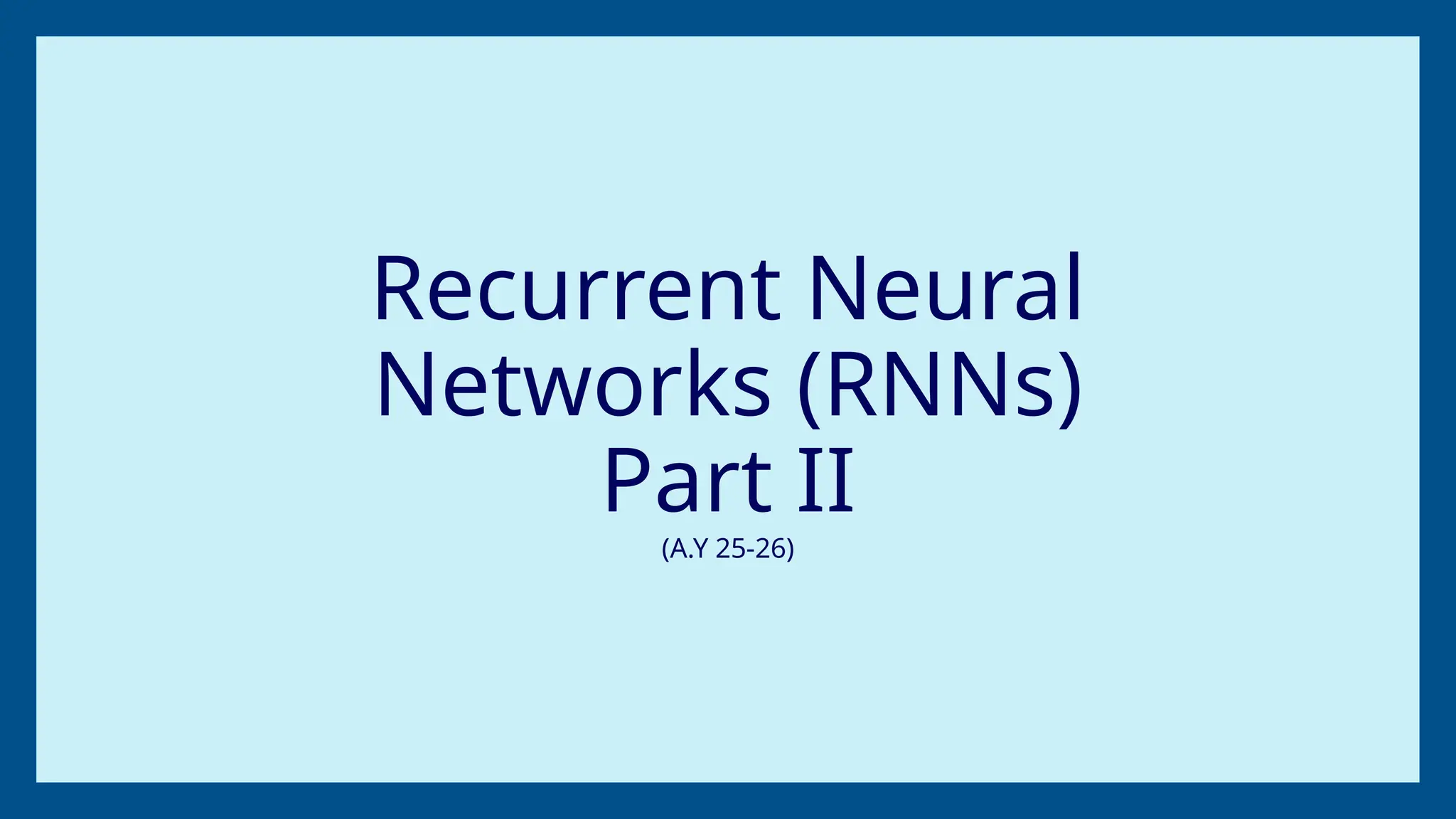
2. What is Sequence Generation?
Sequence generation refers to producing new sequences from an RNN, such as generating
text, music, or other types of sequential data. RNNs are particularly useful here because
they can take in a seed input (e.g., a few starting words or notes) and generate a longer
sequence based on the patterns they've learned.
How Sequence Generation Works with RNNs:
1.Start with a Seed: The RNN is given an initial input (like the first few words of a
sentence or the first note in a musical piece).
2.Generate Next Step: The network predicts the next word or character based on the current
hidden state and input.
3.Feed the Output Back: The output is then fed back into the network as input for the
next time step. This process is repeated, and the sequence grows as the model continues
generating data.
4.Stopping Condition: The generation process continues until a specific condition is
met,such as reaching a maximum length or generating an end token.

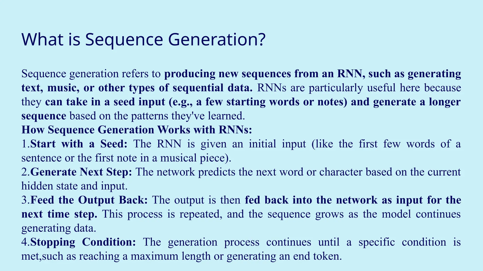
3. What is Sequence Generation?
Example:
1. Starting Input: "Once upon a time"
2. RNN generates the next word: "there"
3. New input: "Once upon a time there"
4. RNN generates the next word: "was"
5. And so on, producing a coherent story: "Once upon a time, there was a little girl."

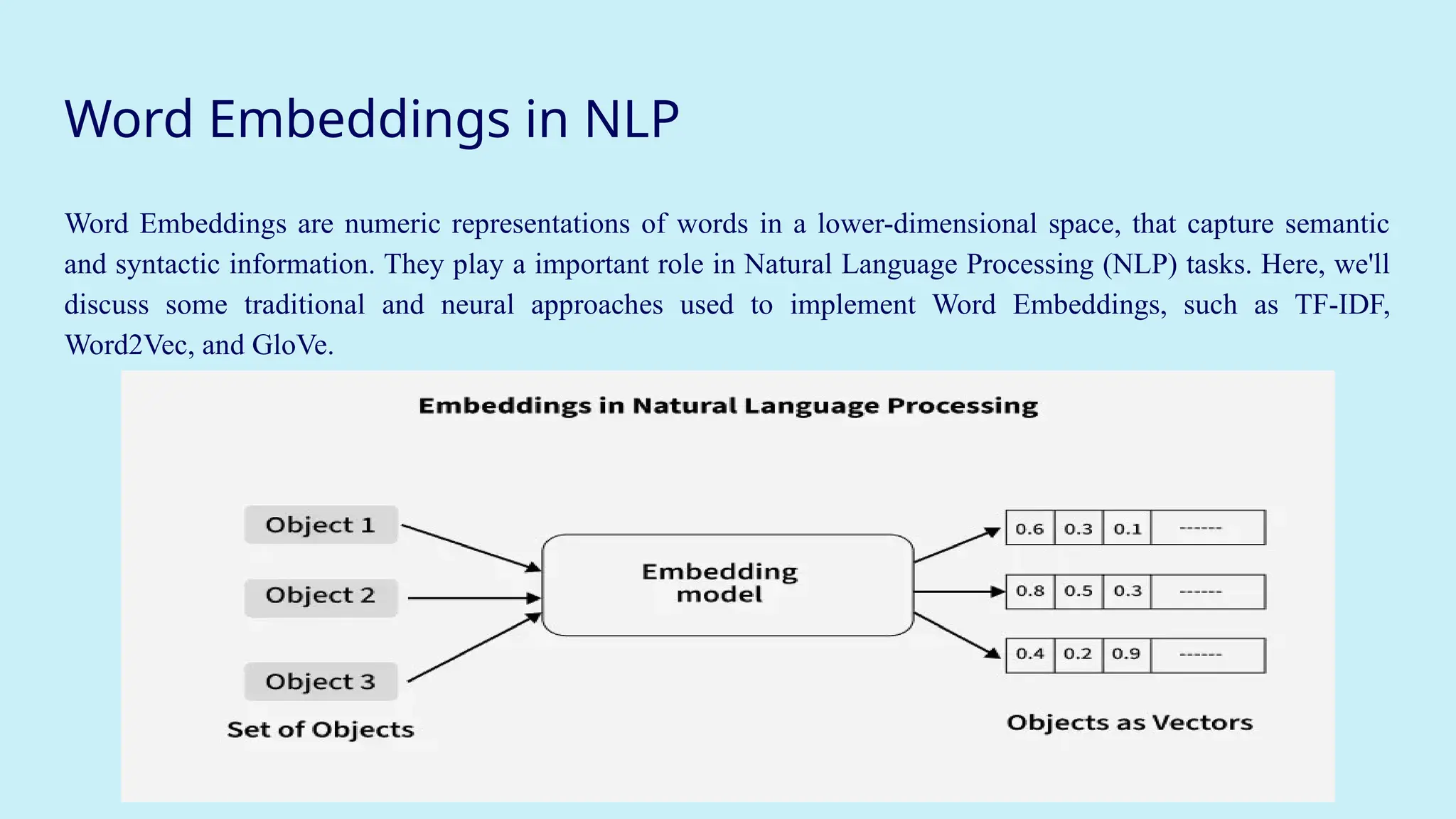
4. Word Embeddings in NLP
Word Embeddings are numeric representations of words in a lower-dimensional space, that capture semantic
and syntactic information. They play a important role in Natural Language Processing (NLP) tasks. Here, we'll
discuss some traditional and neural approaches used to implement Word Embeddings, such as TF-IDF,
Word2Vec, and GloVe.

5. What is Word Embedding in NLP?
Word Embedding is an approach for representing words and documents. Word Embedding or Word
Vector is a numeric vector input that represents a word in a lower-dimensional space.
● Method of extracting features out of text so that we can input those features into a machine
learning model to work with text data.
● It allows words with similar meanings to have a similar representation. Thus, Similarity can
be assessed based on Similar vector representations.
● High Computation Cost: Large input vectors will mean a huge number of weights.
Embeddings help to reduce dimensionality.
● Preserve syntactic and semantic information.
● Some methods based on Word Frequency are Bag of Words (BOW), Countvectorizer and TF-
IDF.

6. Need for Word Embedding?
To reduce dimensionality.
● To use a word to predict the words around it.
● Helps in enhancing model interpretability due to numerical representation.
● Inter-word semantics and similarity can be captured.

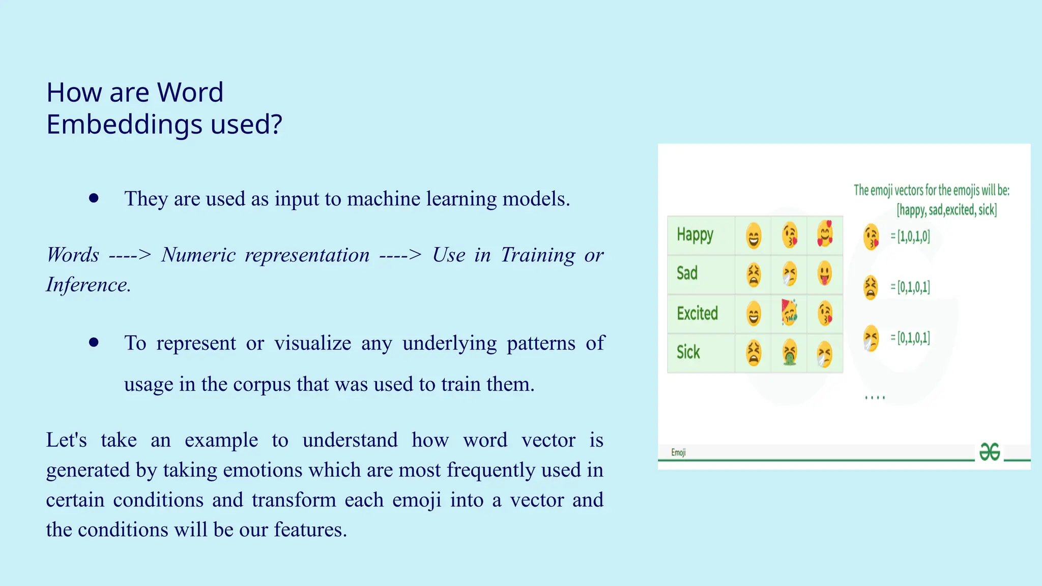
7. How are Word
Embeddings used?
● They are used as input to machine learning models.
Words ----> Numeric representation ----> Use in Training or
Inference.
● To represent or visualize any underlying patterns of
usage in the corpus that was used to train them.
Let's take an example to understand how word vector is
generated by taking emotions which are most frequently used in
certain conditions and transform each emoji into a vector and
the conditions will be our features.

8. Approaches for Text Representation
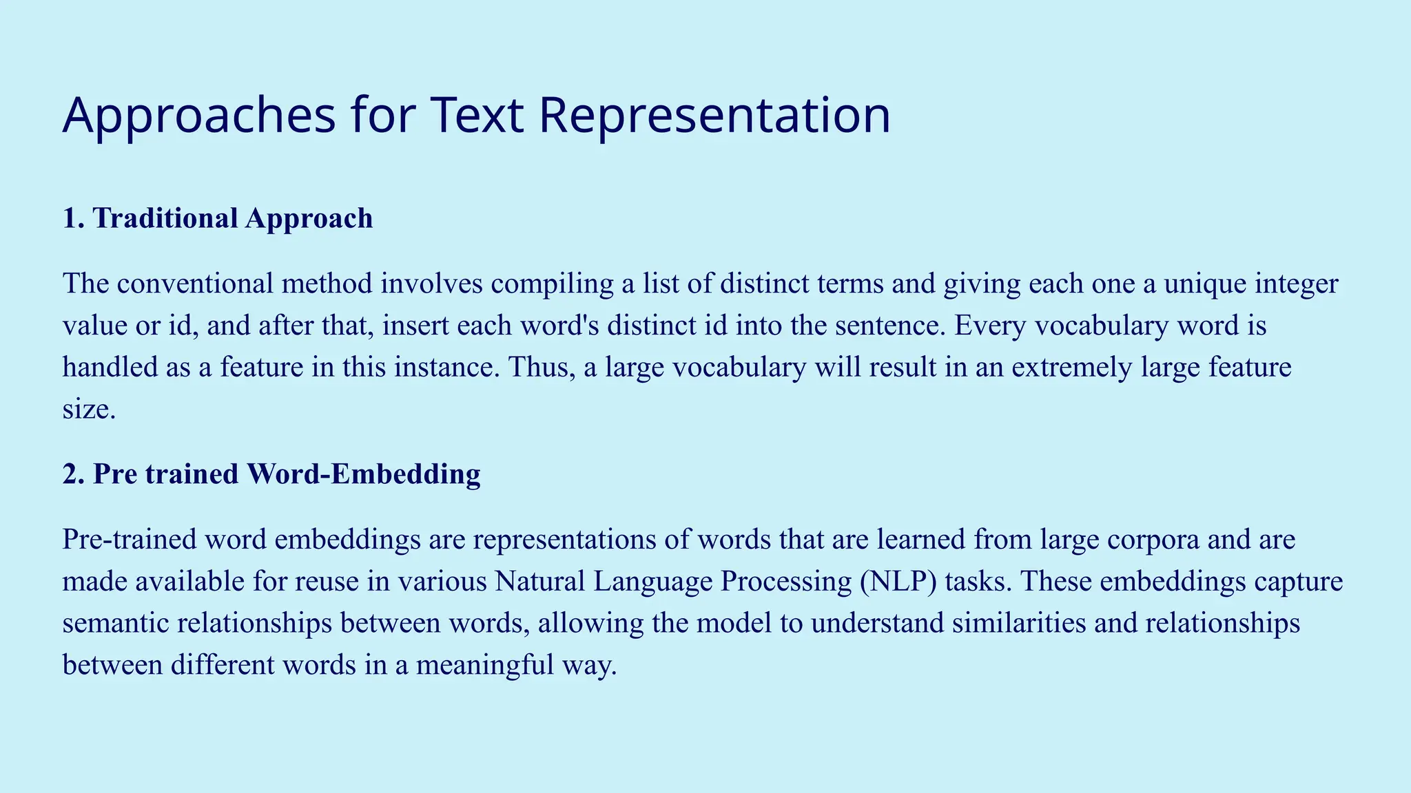
1. Traditional Approach
The conventional method involves compiling a list of distinct terms and giving each one a unique integer
value or id, and after that, insert each word's distinct id into the sentence. Every vocabulary word is
handled as a feature in this instance. Thus, a large vocabulary will result in an extremely large feature
size.
2. Pre trained Word-Embedding
Pre-trained word embeddings are representations of words that are learned from large corpora and are
made available for reuse in various Natural Language Processing (NLP) tasks. These embeddings capture
semantic relationships between words, allowing the model to understand similarities and relationships
between different words in a meaningful way.

9. Sentiment analysis using RNN
Recurrent Neural Networks (RNNs) are used in sequence tasks such as sentiment analysis
due to their ability to capture context from sequential data. The goal is to classify
reviews as positive or negative for providing insights into customer experiences.

10. Sentiment analysis using RNN
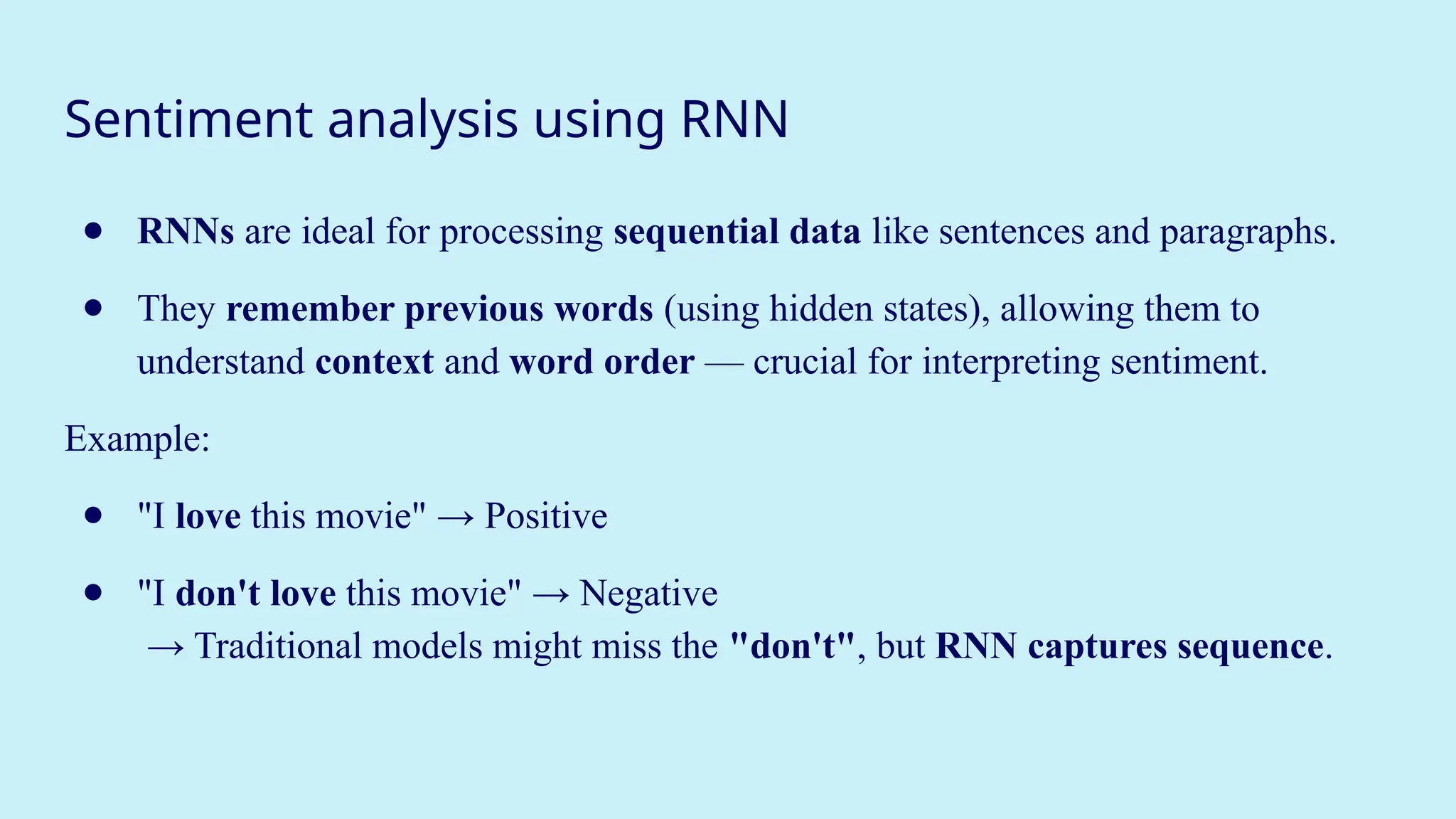
● RNNs are ideal for processing sequential data like sentences and paragraphs.
● They remember previous words (using hidden states), allowing them to
understand context and word order — crucial for interpreting sentiment.
Example:
● "I love this movie" → Positive
● "I don't love this movie" → Negative
→ Traditional models might miss the "don't", but RNN captures sequence.

11. Sentiment analysis using RNN
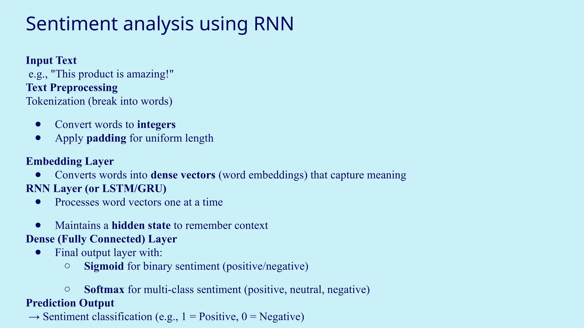
Input Text
e.g., "This product is amazing!"
Text Preprocessing
Tokenization (break into words)
● Convert words to integers
● Apply padding for uniform length
Embedding Layer
● Converts words into dense vectors (word embeddings) that capture meaning
RNN Layer (or LSTM/GRU)
● Processes word vectors one at a time
● Maintains a hidden state to remember context
Dense (Fully Connected) Layer
● Final output layer with:
○ Sigmoid for binary sentiment (positive/negative)
○ Softmax for multi-class sentiment (positive, neutral, negative)
Prediction Output
→ Sentiment classification (e.g., 1 = Positive, 0 = Negative)

12. Text classification using RNN
Text classification is a Natural Language Processing (NLP) task where we assign
predefined categories or labels to a given piece of text.
🟩 Examples:
● Email → "Spam" or "Not Spam"
● News article → "Politics", "Sports", "Technology"
● Tweet → "Hate Speech", "Neutral", "Supportive"

13. Text classification using RNN
Why Use RNN for Text Classification?
● RNNs are designed to work with sequential data like sentences.
● They remember previous words using hidden states, which helps them understand
context.
● Especially useful for:
○ Sentiment analysis
○ Topic classification
○ Intent detection

14. Text classification using RNN
Step-by-Step Workflow
1. Text Preprocessing
● Clean text: remove punctuation, lowercase
● Tokenize: convert words to integers
● Pad sequences to equal length
2. Word Embedding
● Converts tokens into dense vectors
● Captures semantic meaning
● Can use:
○ Pretrained: Word2Vec, GloVe
○ Learned during training

15. Text classification using RNN
3. RNN Layer
● Processes the word vectors one-by-one in sequence
● Maintains a hidden state to remember previous input
Alternatives: Use LSTM or GRU to handle long-term dependencies
4. Fully Connected (Dense) Layer
● Outputs a vector of size equal to number of classes
5. Output Layer
● Sigmoid: for binary classification
● Softmax: for multi-class classification

16. Machine Translation using RNN
Why Neural Networks Need Numbers:
Before using machine translation or neural networks for any language task, we have to convert words
into numbers — because neural networks can only process numbers, not text.

17. Machine Translation using RNN
Tokenization – Turning Text into Numbers
Tokenization is the first step:
● It breaks text into words or subwords (called tokens).
● Removes punctuation, applies stemming (e.g., "running" → "run"), and converts
everything to lowercase.
● Then assigns each word a unique number (a token).
Example:
Sentence: "The cat sat."
After tokenization: {"the": 1, "cat": 2, "sat": 3}
Now your model can work with [1, 2, 3] instead of ["The", "cat", "sat"].

18. Machine Translation using RNN
Recurrent Neural Networks (RNNs): Why We Use Them
Normal neural networks don't remember previous inputs. But language is sequential — the meaning of a word
depends on the words before it.
RNNs solve this by introducing memory.
● At each time step t, an RNN takes:
○ the current word (x[t])
○ the previous memory state (a[t-1])
○ and produces a new memory state (a[t]) and maybe an output (y[t])
This lets the network “remember” earlier words.

19. Machine Translation using RNN
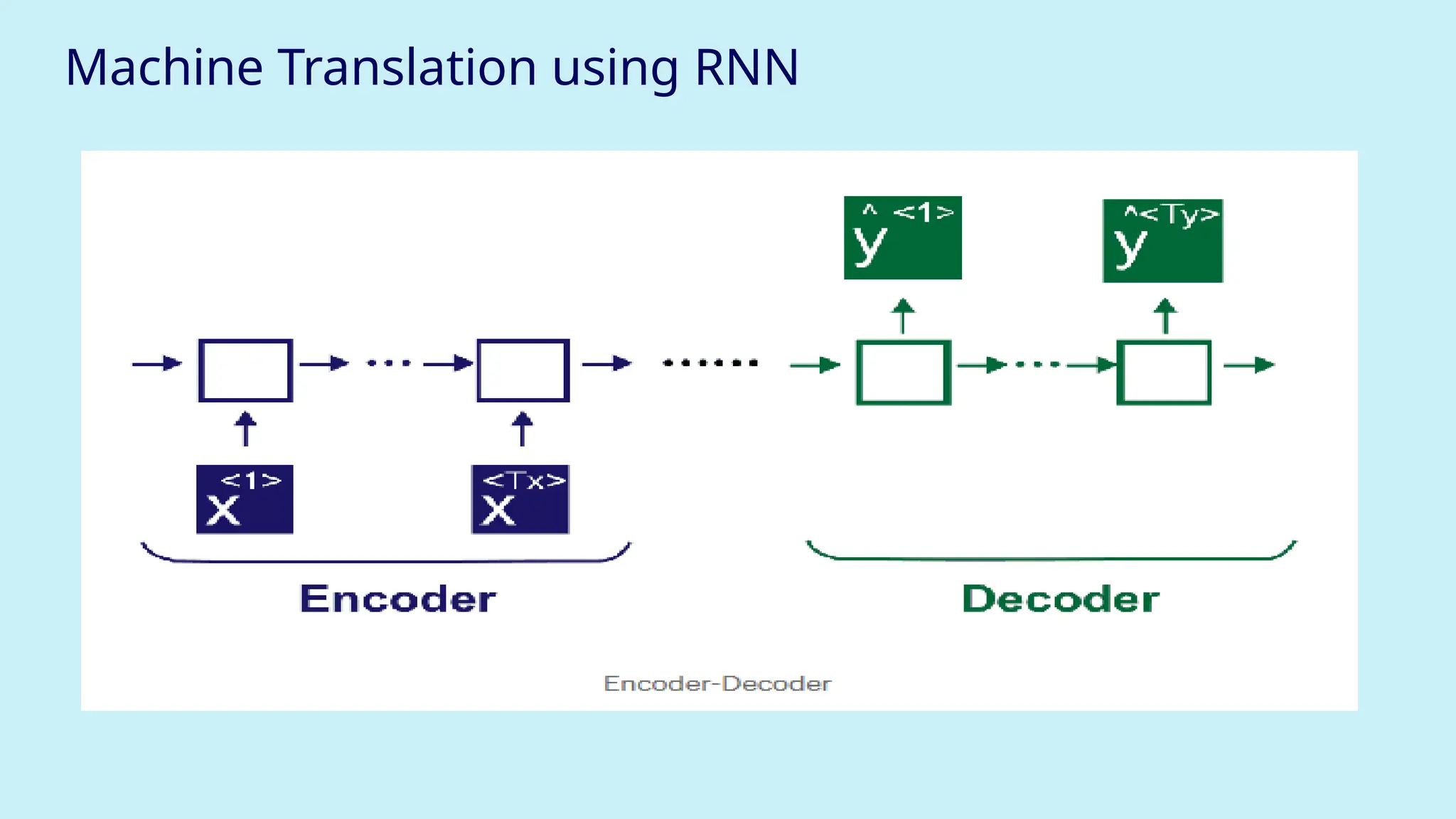
Machine Translation: Encoder–Decoder Architecture
When translating a sentence from one language to another (like English to Hindi), we use two
RNNs:
Encoder:
● Takes the input sentence (e.g., "What is your name") word by word.
● Converts it into a summary vector (called the context vector).
● This vector contains the meaning of the whole sentence.
Decoder:
● Takes this context vector and generates the output sentence (e.g., "Aapka naam kya hai") one
word at a time.

20. Machine Translation using RNN

21. Machine Translation using RNN
Inside the RNN Cell (Mathematics)
Forward Propagation Equations:
a[t] = tanh(Waa * a[t-1] + Wax * x[t] + ba) # Hidden state
y[t] = softmax(Wya * a[t] + by) # Output
Waa: weight for previous activation
Wax: weight for current input
ba, by: bias terms
a[t]: current memory (hidden) state
y[t]: prediction/output at time t
This structure allows RNNs to share learned features across time steps, like learning that
"am" often follows "I".

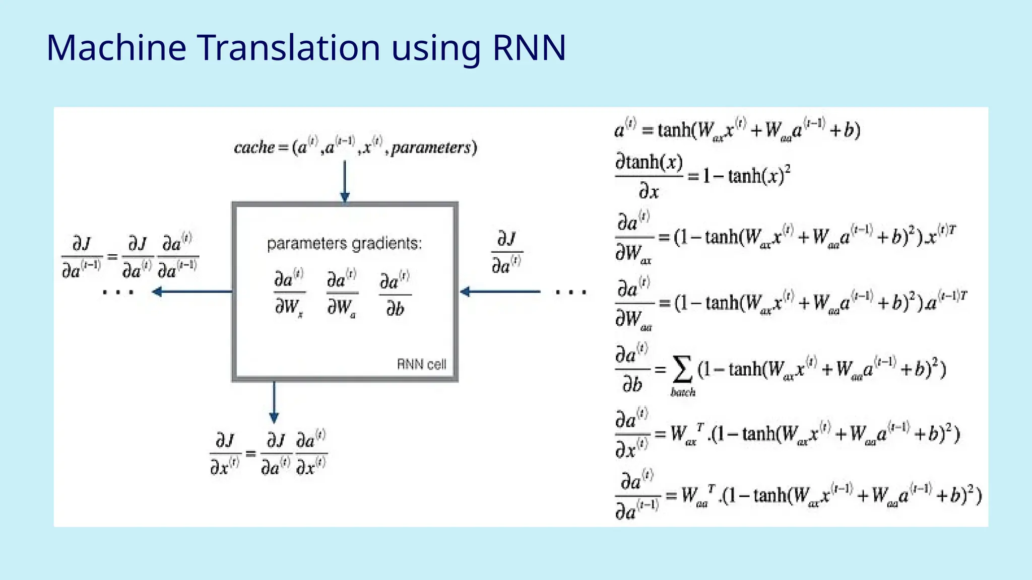
22. Machine Translation using RNN
RNN Unrolled (Over Time Steps)
Each state passes its memory to the next, forming a chain.
Time t=0: x[0] → a[0]
Time t=1: x[1] + a[0] → a[1]
Time t=2: x[2] + a[1] → a[2]

23. Machine Translation using RNN
Backpropagation Through Time (BPTT)
Just like we do forward pass, we also do backward pass to update weights using errors.
But since an RNN is a chain, we must propagate errors through all time steps.
● This involves computing derivatives of the loss with respect to each weight (Waa,
Wax, etc.)
● To avoid re-computing, we use a cache to store useful values.

24. Machine Translation using RNN

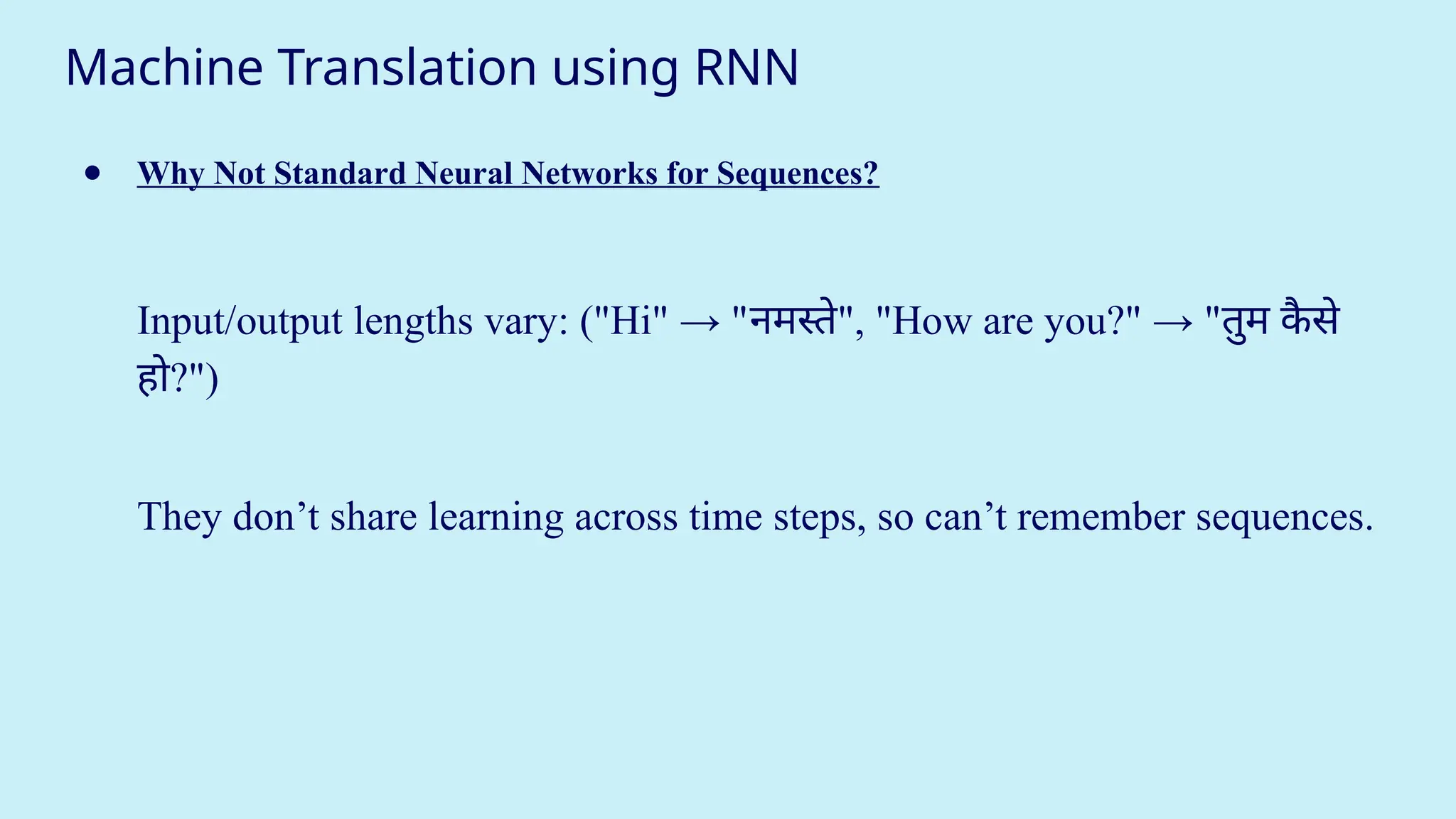
25. Machine Translation using RNN
● Why Not Standard Neural Networks for Sequences?
Input/output lengths vary: ("Hi" → "नमस्ते", "How are you?" → "तुम क
ै से
हो?")
They don’t share learning across time steps, so can’t remember sequences.

26. Machine Translation using RNN
Example of Encoder–Decoder in Action
English Sentence (Input): "What is your name?"
Hindi Sentence (Output): "Aapka naam kya hai"
Encoder:
1. "What" → embeds → RNN cell → a[0]
2. "is" → embeds + a[0] → a[1]
3. "your" → embeds + a[1]→ a[2]
4. "name" → embeds + a[2] → final context vector
Decoder:
5. Context vector → RNN → "Aapka"
6. "Aapka" + RNN → "naam"
7. … and so on

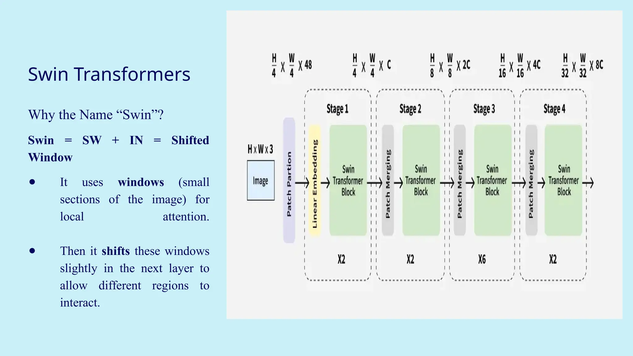
27. Swin Transformers
Why the Name “Swin”?
Swin = SW + IN = Shifted
Window
● It uses windows (small
sections of the image) for
local attention.
● Then it shifts these windows
slightly in the next layer to
allow different regions to
interact.

28. Swin Transformers
Basic Structure of Swin Transformer
Here’s a step-by-step overview of how it works.
1. Patch Splitting
● The image is cut into small patches (like dividing a photo into small tiles).
● Each patch is turned into a vector (numbers) — this is your input to the model.
Example: A 224 x 224 image split into 4 x 4 patches → 56 x 56 patches in total.

29. Swin Transformers
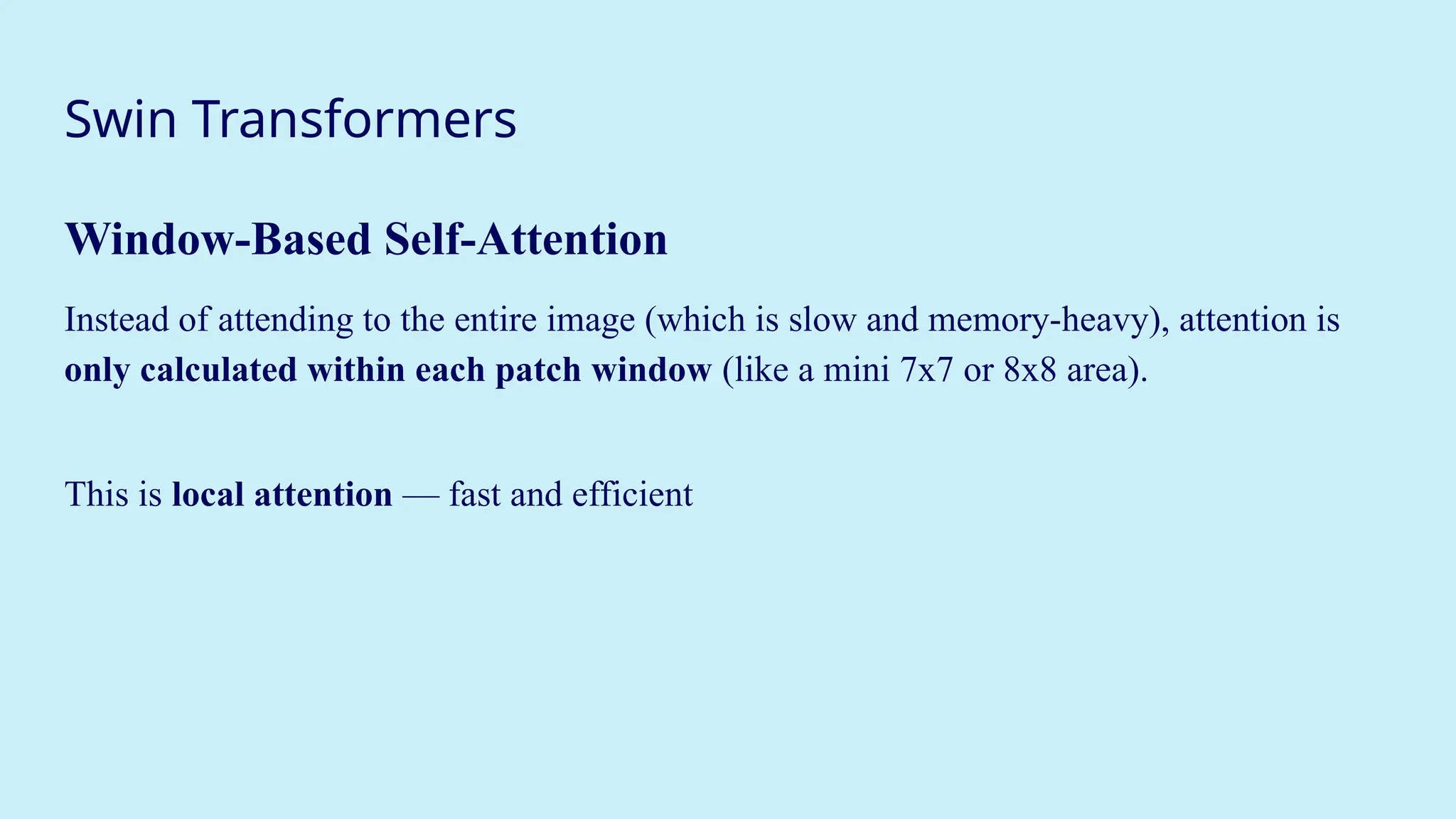
Window-Based Self-Attention
Instead of attending to the entire image (which is slow and memory-heavy), attention is
only calculated within each patch window (like a mini 7x7 or 8x8 area).
This is local attention — fast and efficient

30. Swin Transformers
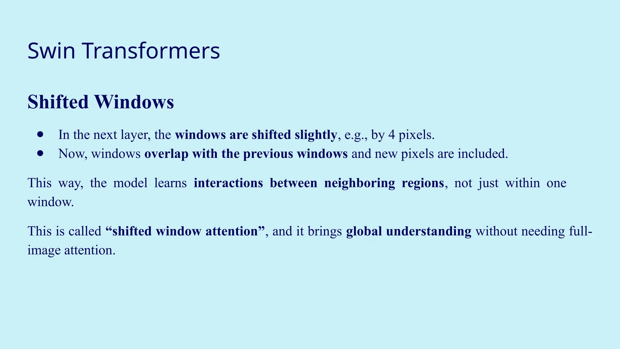
Shifted Windows
● In the next layer, the windows are shifted slightly, e.g., by 4 pixels.
● Now, windows overlap with the previous windows and new pixels are included.
This way, the model learns interactions between neighboring regions, not just within one
window.
This is called “shifted window attention”, and it brings global understanding without needing full-
image attention.

31. Swin Transformers
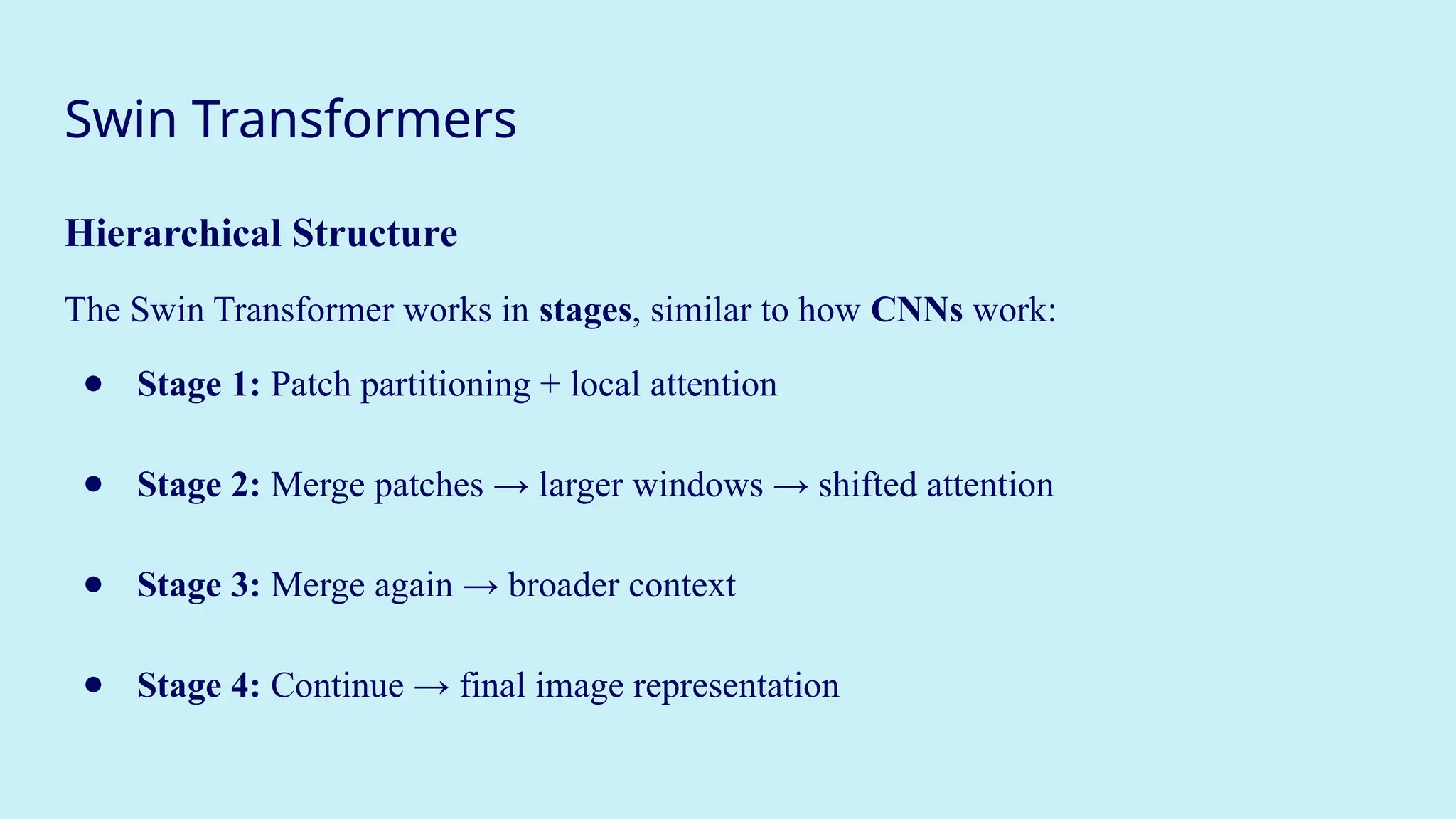
Hierarchical Structure
The Swin Transformer works in stages, similar to how CNNs work:
● Stage 1: Patch partitioning + local attention
● Stage 2: Merge patches → larger windows → shifted attention
● Stage 3: Merge again → broader context
● Stage 4: Continue → final image representation

32. Swin Transformers
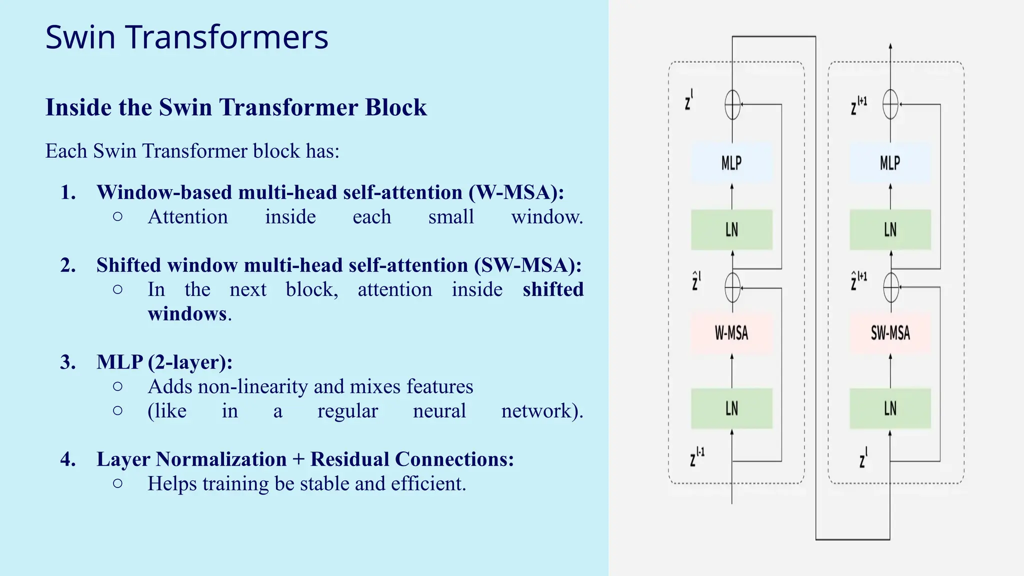
Inside the Swin Transformer Block
Each Swin Transformer block has:
1. Window-based multi-head self-attention (W-MSA):
○ Attention inside each small window.
2. Shifted window multi-head self-attention (SW-MSA):
○ In the next block, attention inside shifted
windows.
3. MLP (2-layer):
○ Adds non-linearity and mixes features
○ (like in a regular neural network).
4. Layer Normalization + Residual Connections:
○ Helps training be stable and efficient.

33. Performer, and Vision Transformers (ViT) for
efficient computations.

34. Performer, and Vision Transformers (ViT) for
efficient computations.
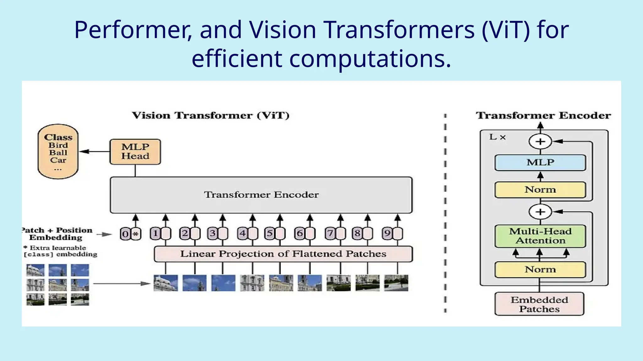
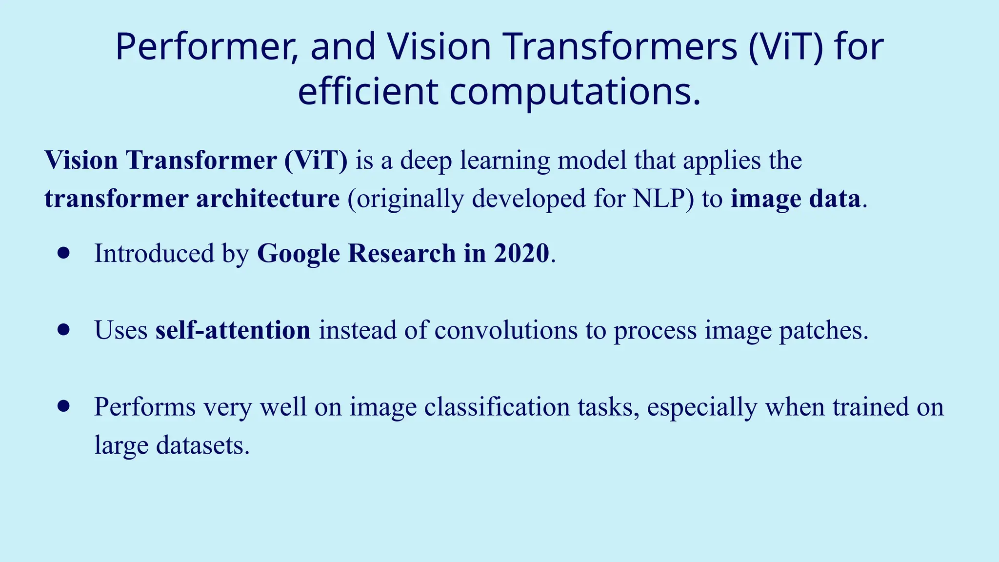
Vision Transformer (ViT) is a deep learning model that applies the
transformer architecture (originally developed for NLP) to image data.
● Introduced by Google Research in 2020.
● Uses self-attention instead of convolutions to process image patches.
● Performs very well on image classification tasks, especially when trained on
large datasets.

35. Performer, and Vision Transformers (ViT) for
efficient computations.
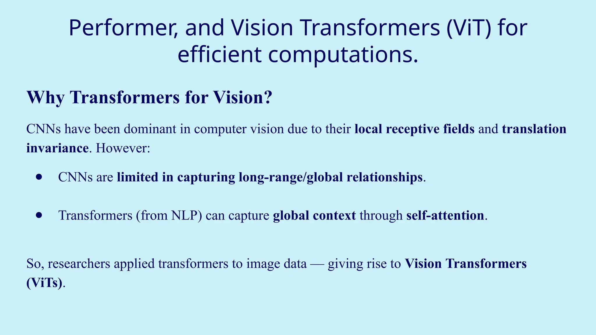
Why Transformers for Vision?
CNNs have been dominant in computer vision due to their local receptive fields and translation
invariance. However:
● CNNs are limited in capturing long-range/global relationships.
● Transformers (from NLP) can capture global context through self-attention.
So, researchers applied transformers to image data — giving rise to Vision Transformers
(ViTs).

36. Performer, and Vision Transformers (ViT) for
efficient computations.
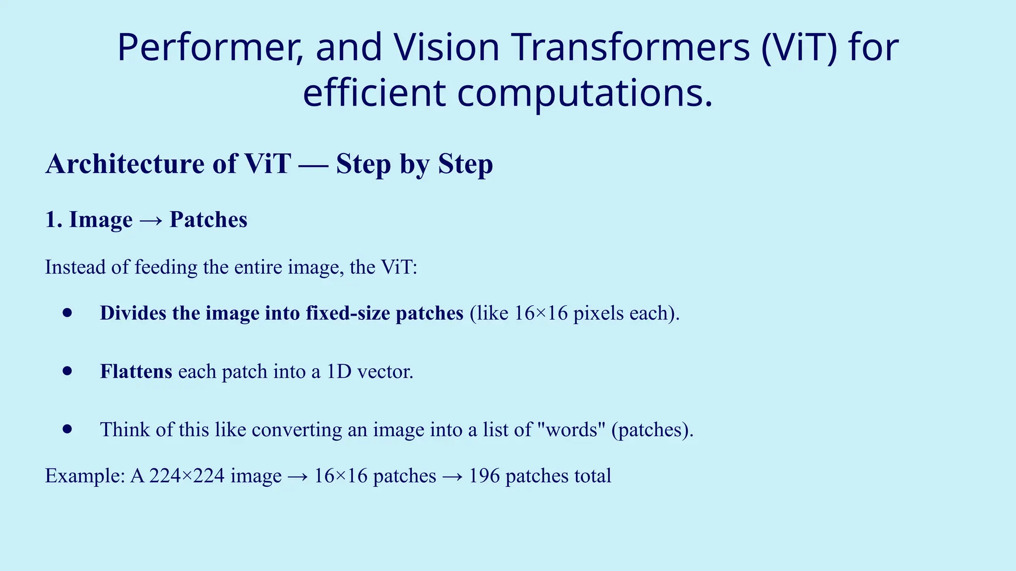
Architecture of ViT — Step by Step
1. Image → Patches
Instead of feeding the entire image, the ViT:
● Divides the image into fixed-size patches (like 16×16 pixels each).
● Flattens each patch into a 1D vector.
● Think of this like converting an image into a list of "words" (patches).
Example: A 224×224 image → 16×16 patches → 196 patches total

37. Performer, and Vision Transformers (ViT) for
efficient computations.
Patch Embedding
Each patch is passed through a linear embedding layer:
● Each 2D patch (16×16×3) is flattened into a vector.
● Then passed through a fully connected layer → patch embedding.
These embeddings are just like word embeddings in NLP.

38. Performer, and Vision Transformers (ViT) for
efficient computations.
Linear Projection (Flatten + Embed)
"Turn each patch into a number vector."
● Each 16×16 patch has pixel values (e.g., RGB).
● You flatten this 2D patch into a 1D vector (e.g., length 768).
● Then, use a linear layer (a small neural network) to convert it into an
embedding vector (say of size 512 or 768).

39. Performer, and Vision Transformers (ViT) for
efficient computations.
Add Position Embeddings
Why? Transformers process all tokens in parallel and don’t know where the patch
came from (top-left, bottom-right, etc.).
To fix this:
● Add a position encoding vector to each patch embedding.
● This encodes spatial location — like saying:
"This patch came from row 1, column 2"

40. Performer, and Vision Transformers (ViT) for
efficient computations.
Transformer Encoder Layers
● The self-attention mechanism allows each patch to look at all other patches.
● For example:
○ Patch with the car wheel learns from patch with car body
○ Patch with dog's nose learns from patch with dog’s ear
This builds a global understanding of the whole image — the patches share
knowledge.

41. Performer, and Vision Transformers (ViT) for
efficient computations.
Add Classification Token ([CLS])
"A special token that summarizes the whole image."
● Add a special extra token at the beginning — called the [CLS] token (like in
BERT).
● As the transformer layers run, this token collects and mixes information
from all other patches.
At the end, this [CLS] token contains the summary of the entire image — like an
overall impression.

42. Performer, and Vision Transformers (ViT) for
efficient computations.
Final Classification
"Predict what’s in the image."
● Pass the [CLS] token through a final simple neural network (MLP
head).
● The output gives the class label:
E.g., “dog”, “cat”, “car”, “airplane” etc.