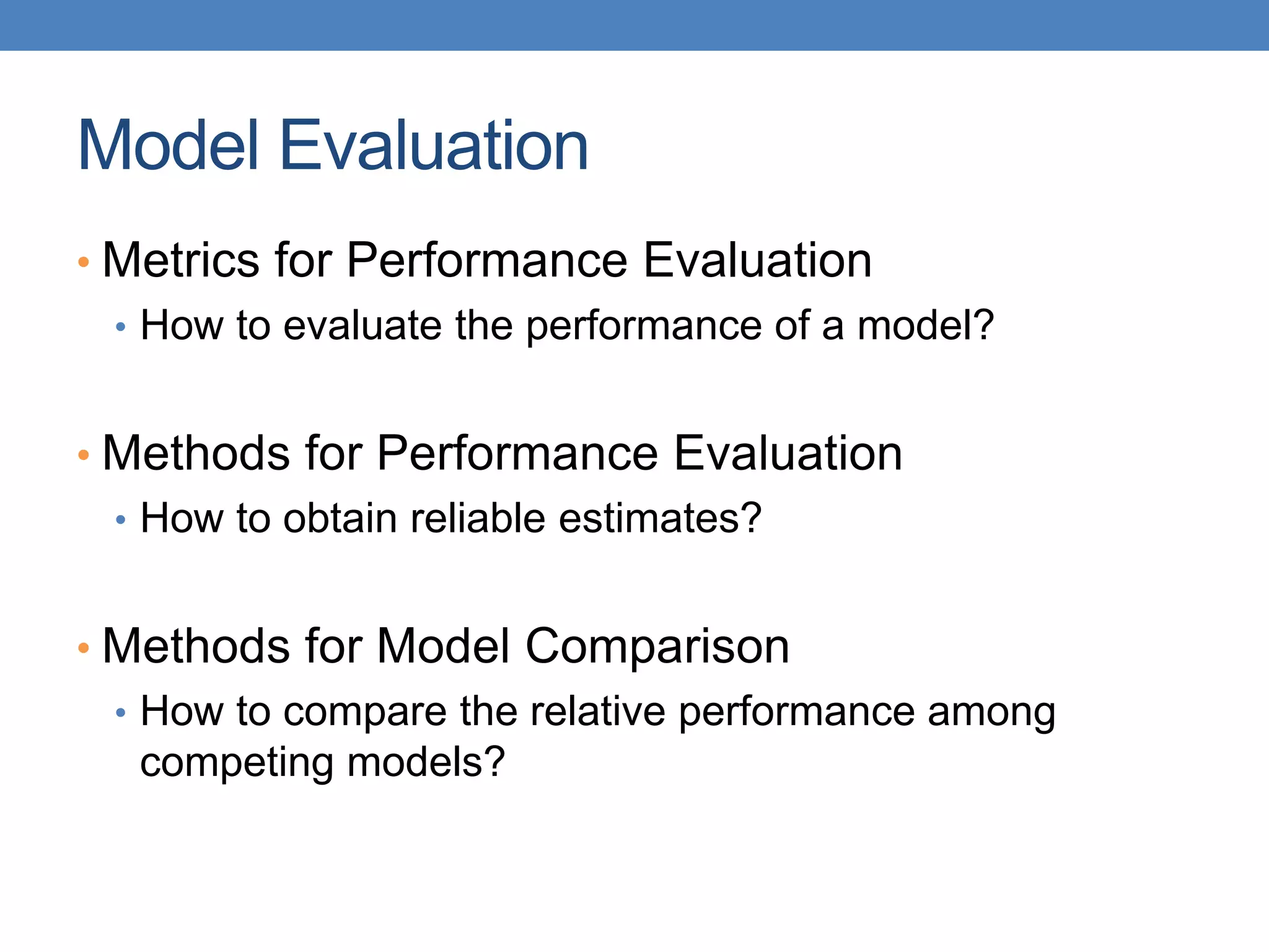
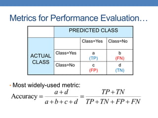
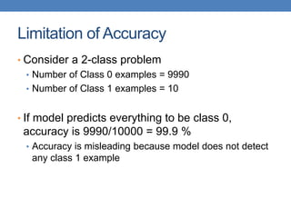
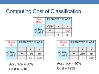
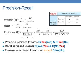
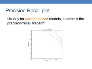
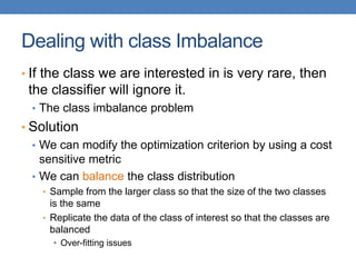
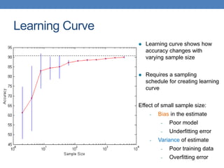
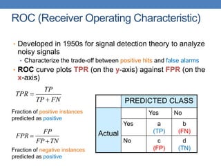
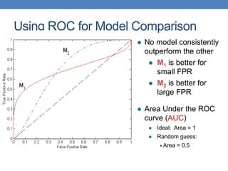
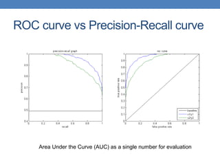
The document discusses various methods for evaluating machine learning models and comparing their performance. It covers metrics like accuracy, precision, recall, cost matrices, and ROC curves. Key methods discussed include holdout validation, k-fold cross validation, and the bootstrap method for obtaining reliable performance estimates. It also addresses issues like class imbalance and overfitting. ROC curves and the area under the ROC curve are presented as ways to visually and quantitatively compare models.

1. Model Evaluation
• Metrics for Performance Evaluation
• How to evaluate the performance of a model?
• Methods for Performance Evaluation
• How to obtain reliable estimates?
• Methods for Model Comparison
• How to compare the relative performance among
competing models?

2. Model Evaluation
• Metrics for Performance Evaluation
• How to evaluate the performance of a model?
• Methods for Performance Evaluation
• How to obtain reliable estimates?
• Methods for Model Comparison
• How to compare the relative performance among
competing models?

3. Metrics for Performance Evaluation
• Focus on the predictive capability of a model
• Rather than how fast it takes to classify or build models,
scalability, etc.
• Confusion Matrix:
PREDICTED CLASS
ACTUAL
CLASS
Class=Yes Class=No
Class=Yes a b
Class=No c d
a: TP (true positive)
b: FN (false negative)
c: FP (false positive)
d: TN (true negative)

4. Metrics for Performance Evaluation…
• Most widely-used metric:
PREDICTED CLASS
ACTUAL
CLASS
Class=Yes Class=No
Class=Yes a
(TP)
b
(FN)
Class=No c
(FP)
d
(TN)
FN
FP
TN
TP
TN
TP
d
c
b
a
d
a










Accuracy

5. Limitation of Accuracy
• Consider a 2-class problem
• Number of Class 0 examples = 9990
• Number of Class 1 examples = 10
• If model predicts everything to be class 0,
accuracy is 9990/10000 = 99.9 %
• Accuracy is misleading because model does not detect
any class 1 example

6. Cost Matrix
PREDICTED CLASS
ACTUAL
CLASS
C(i|j) Class=Yes Class=No
Class=Yes C(Yes|Yes) C(No|Yes)
Class=No C(Yes|No) C(No|No)
C(i|j): Cost of classifying class j example as class i
d
w
c
w
b
w
a
w
d
w
a
w
4
3
2
1
4
1
Accuracy
Weighted






7. Computing Cost of Classification
Cost
Matrix
PREDICTED CLASS
ACTUAL
CLASS
C(i|j) + -
+ -1 100
- 1 0
Model
M1
PREDICTED CLASS
ACTUAL
CLASS
+ -
+ 150 40
- 60 250
Model
M2
PREDICTED CLASS
ACTUAL
CLASS
+ -
+ 250 45
- 5 200
Accuracy = 80%
Cost = 3910
Accuracy = 90%
Cost = 4255

8. Cost vs Accuracy
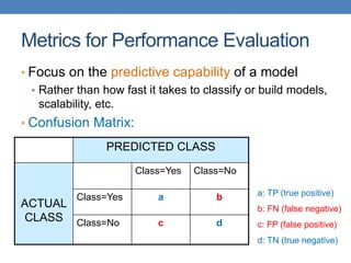
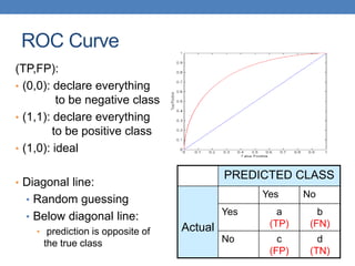
Count PREDICTED CLASS
ACTUAL
CLASS
Class=Yes Class=No
Class=Yes a b
Class=No c d
Cost PREDICTED CLASS
ACTUAL
CLASS
Class=Yes Class=No
Class=Yes p q
Class=No q p
N = a + b + c + d
Accuracy = (a + d)/N
Cost = p (a + d) + q (b + c)
= p (a + d) + q (N – a – d)
= q N – (q – p)(a + d)
= N [q – (q-p)  Accuracy]
Accuracy is proportional to cost if
1. C(Yes|No)=C(No|Yes) = q
2. C(Yes|Yes)=C(No|No) = p

9. Precision-Recall
FN
FP
TP
TP
c
b
a
a
p
r
rp
p
r
FN
TP
TP
b
a
a
FP
TP
TP
c
a
a













 









2
2
2
2
2
2
/
1
/
1
1
(F)
measure
-
F
(r)
Recall
(p)
Precision
 Precision is biased towards C(Yes|Yes) & C(Yes|No)
 Recall is biased towards C(Yes|Yes) & C(No|Yes)
 F-measure is biased towards all except C(No|No)
Count PREDICTED CLASS
ACTUAL
CLASS
Class=Yes Class=No
Class=Yes a b
Class=No c d

10. Precision-Recall plot
• Usually for parameterized models, it controls the
precision/recall tradeoff

11. Model Evaluation
• Metrics for Performance Evaluation
• How to evaluate the performance of a model?
• Methods for Performance Evaluation
• How to obtain reliable estimates?
• Methods for Model Comparison
• How to compare the relative performance among
competing models?

12. Methods for Performance Evaluation
• How to obtain a reliable estimate of
performance?
• Performance of a model may depend on other
factors besides the learning algorithm:
• Class distribution
• Cost of misclassification
• Size of training and test sets

13. Methods of Estimation
• Holdout
• Reserve 2/3 for training and 1/3 for testing
• Random subsampling
• One sample may be biased -- Repeated holdout
• Cross validation
• Partition data into k disjoint subsets
• k-fold: train on k-1 partitions, test on the remaining one
• Leave-one-out: k=n
• Guarantees that each record is used the same number of
times for training and testing
• Bootstrap
• Sampling with replacement
• ~63% of records used for training, ~27% for testing

14. Dealing with class Imbalance
• If the class we are interested in is very rare, then
the classifier will ignore it.
• The class imbalance problem
• Solution
• We can modify the optimization criterion by using a cost
sensitive metric
• We can balance the class distribution
• Sample from the larger class so that the size of the two classes
is the same
• Replicate the data of the class of interest so that the classes are
balanced
• Over-fitting issues

15. Learning Curve
 Learning curve shows how
accuracy changes with
varying sample size
 Requires a sampling
schedule for creating learning
curve
Effect of small sample size:
- Bias in the estimate
- Poor model
- Underfitting error
- Variance of estimate
- Poor training data
- Overfitting error

16. Model Evaluation
• Metrics for Performance Evaluation
• How to evaluate the performance of a model?
• Methods for Performance Evaluation
• How to obtain reliable estimates?
• Methods for Model Comparison
• How to compare the relative performance among
competing models?

17. ROC (Receiver Operating Characteristic)
• Developed in 1950s for signal detection theory to analyze
noisy signals
• Characterize the trade-off between positive hits and false alarms
• ROC curve plots TPR (on the y-axis) against FPR (on the
x-axis)
FN
TP
TP
TPR


TN
FP
FP
FPR


PREDICTED CLASS
Actual
Yes No
Yes a
(TP)
b
(FN)
No c
(FP)
d
(TN)
Fraction of positive instances
predicted as positive
Fraction of negative instances
predicted as positive

18. ROC (Receiver Operating Characteristic)
• Performance of a classifier represented as a point
on the ROC curve
• Changing some parameter of the algorithm,
sample distribution, or cost matrix changes the
location of the point

19. ROC Curve
At threshold t:
TP=0.5, FN=0.5, FP=0.12, FN=0.88
- 1-dimensional data set containing 2 classes (positive and negative)
- any points located at x > t is classified as positive

20. ROC Curve
(TP,FP):
• (0,0): declare everything
to be negative class
• (1,1): declare everything
to be positive class
• (1,0): ideal
• Diagonal line:
• Random guessing
• Below diagonal line:
• prediction is opposite of
the true class
PREDICTED CLASS
Actual
Yes No
Yes a
(TP)
b
(FN)
No c
(FP)
d
(TN)

21. Using ROC for Model Comparison
 No model consistently
outperform the other
 M1 is better for
small FPR
 M2 is better for
large FPR
 Area Under the ROC
curve (AUC)
 Ideal: Area = 1
 Random guess:
 Area = 0.5

22. ROC curve vs Precision-Recall curve
Area Under the Curve (AUC) as a single number for evaluation