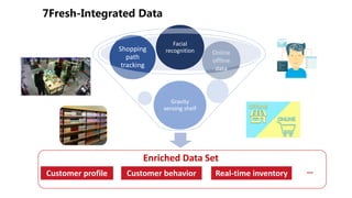
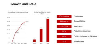
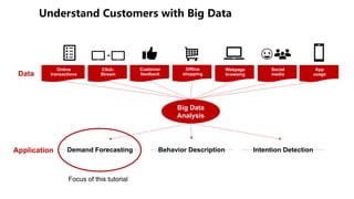
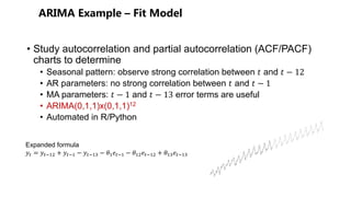
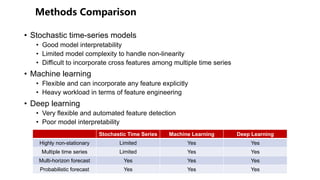
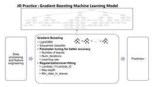
The document discusses the role of data science in retail-as-a-service, highlighting the importance of understanding, connecting with, and serving customers effectively. It emphasizes the growth of online retail in China, the strategic partnerships of major companies, and the use of advanced analytics and technology for demand forecasting and customer behavior analysis. Furthermore, it outlines various modeling techniques, including machine learning and time series models, to address complex supply chain and customer needs challenges.


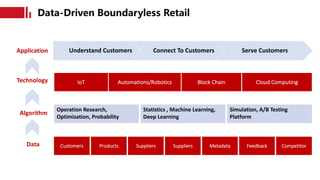


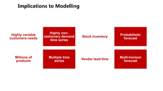

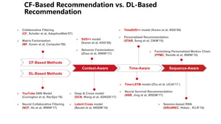
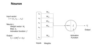
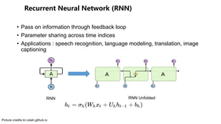
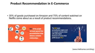
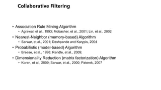
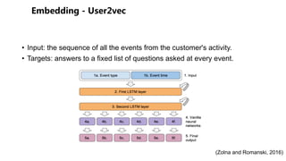
![Time series
Category,
subcategory, brand,
color, shape, size
Day of the
week, lunar
week, hour of
the day,
3-digit zip code
Local
festival
Promotional
events
SKU Attributes LocationTime
Sales Data
Human Expert EmbeddingOne Hot Encoding Feature Hashing
Features
Example features
Mean of the past 7-day sales
Variance of the past 7-day sales
Max sales of the past 14 days
Sales the 7th day in the past
90% sales quantile of last month
Example features
Festival encoding ([0,0,0,1,0,0])
Percentage of discount
Promotional type (hash id)
Category (hash id)
SKU Name (embedding vector)](https://image.slidesharecdn.com/kdd-tutorial-website-180817024123/85/Data-Science-in-Retail-as-a-Service-30-320.jpg)
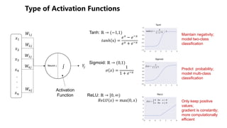
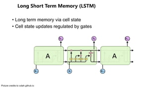


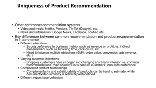

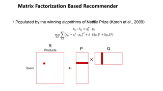

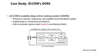
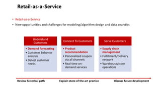
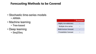
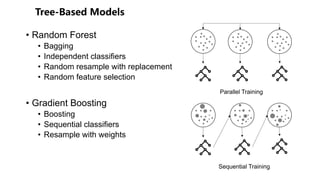
![+ -
Input Layer
Embedding
Layer
Recurrent
Layers
Fully-
Connected
Layers
Output Layer
Cross-product Transform
Memorization+Generalization
Wide&Deep
[DLRS 16]
Embedding Concatenation
YouTube
[RecSys 16]
! = #$ ∗ #′ ∗ ' + ) + #
DCN Deep&Cross
[ADKDD 17]](https://image.slidesharecdn.com/kdd-tutorial-website-180817024123/85/Data-Science-in-Retail-as-a-Service-68-320.jpg)
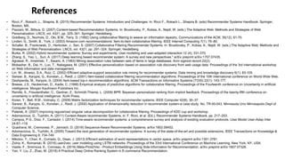
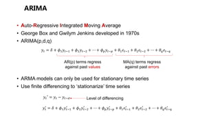
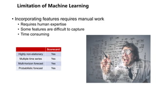
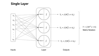
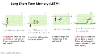
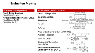
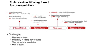
![+
Input Layer
Embedding
Layer
Recurrent
Layers
Fully-
Connected
Layers
Output Layer
Cross-product Transform
Memorization+Generalization
Wide&Deep
[DLRS 16]
Embedding Concatenation
YouTube
[RecSys 16]
ℎ(#)
= 1 + () + (* ∗ ℎ(#)
Latent Cross
[WSDM 18]
Updating Gating Mechanism:
h) = -./0(ℎ)12, 4))
RRN
[WSDM 17]
Gating Mechanism:
+time gates(Phased-LSTM)
Time-LSTM
[IJCAI 17]
5 = 67 ∗ 6′ ∗ ( + 9 + 6
DCN Deep&Cross
[ADKDD 17]
Multi-task Training LSTM
Ob Func: negative Poisson log-likelihood
NSR
[WSDM 17]](https://image.slidesharecdn.com/kdd-tutorial-website-180817024123/85/Data-Science-in-Retail-as-a-Service-69-320.jpg)
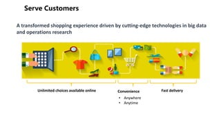
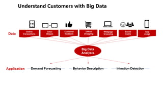
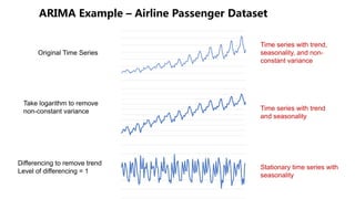
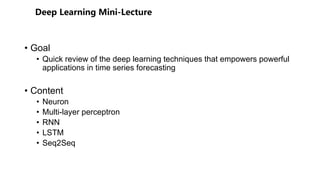
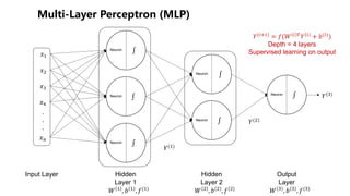
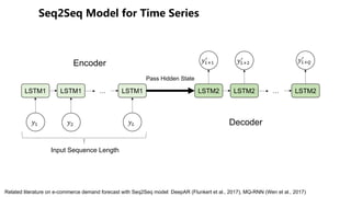
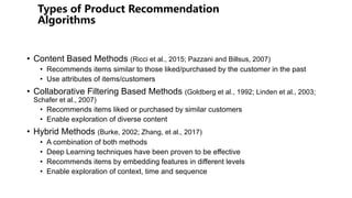
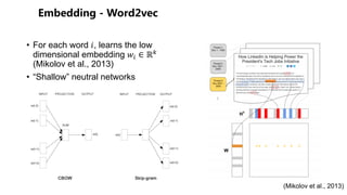
![- +
Input Layer
Embedding
Layer
Recurrent
Layers
Fully-
Connected
Layers
Output Layer
Cross-product Transform
Memorization+Generalization
Wide&Deep
[DLRS 16]
Embedding Concatenation
YouTube
[RecSys 16]
ℎ(#)
= 1 + () + (* ∗ ℎ(#)
Latent Cross
[WSDM 18]
Updating Gating Mechanism:
h) = -./0(ℎ)12, 4))
RRN
[WSDM 17]
Gating Mechanism:
+time gates(Phased-LSTM)
Time-LSTM
[IJCAI 17]
Session Sequence Embedding
GRU4REC
[ICLR 16]
5 = 67 ∗ 6′ ∗ ( + 9 + 6
DCN Deep&Cross
[ADKDD 17]
Multi-task Training LSTM
Ob Func: negative Poisson log-likelihood
NSR
[WSDM 17]](https://image.slidesharecdn.com/kdd-tutorial-website-180817024123/85/Data-Science-in-Retail-as-a-Service-70-320.jpg)