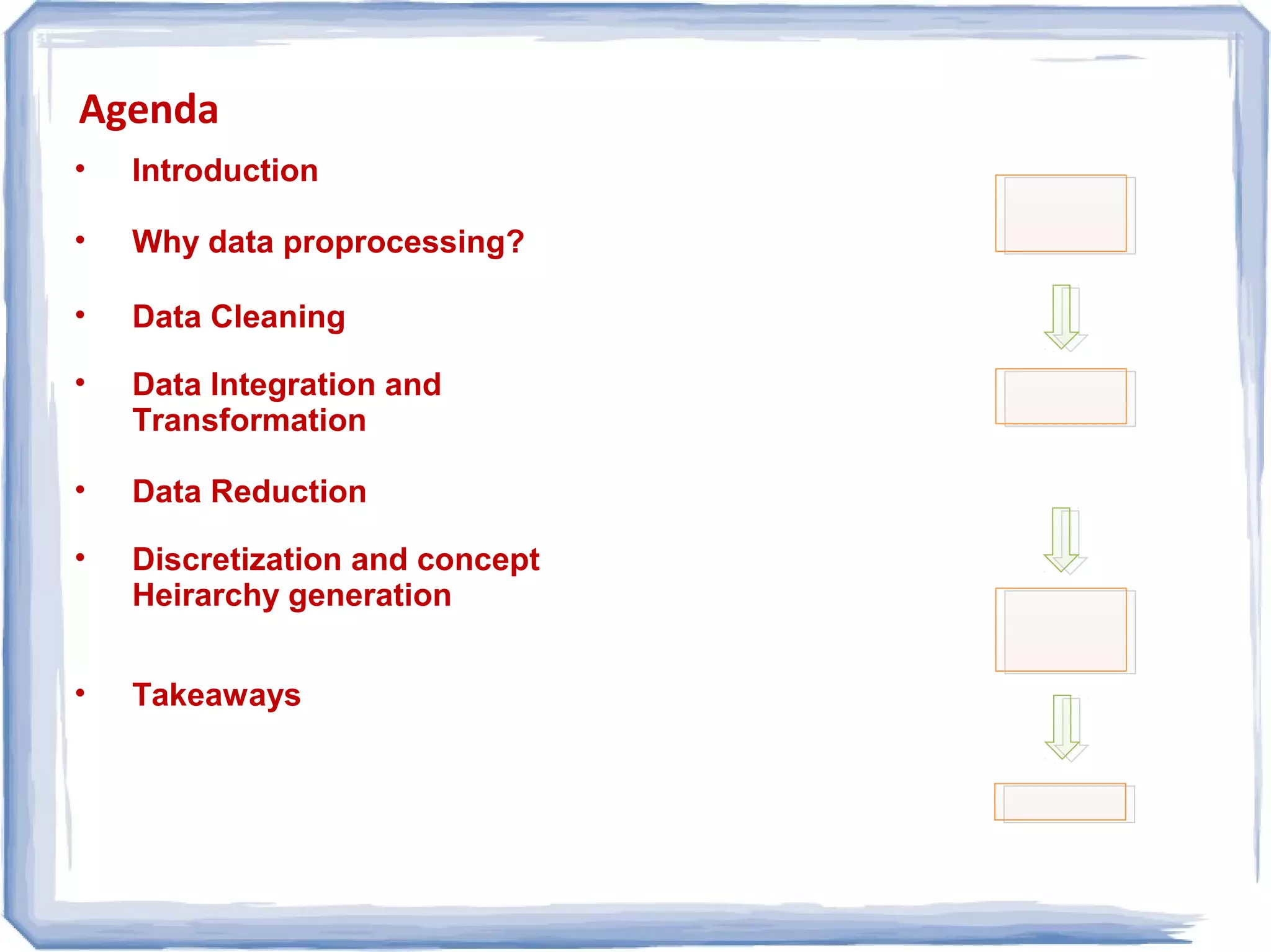
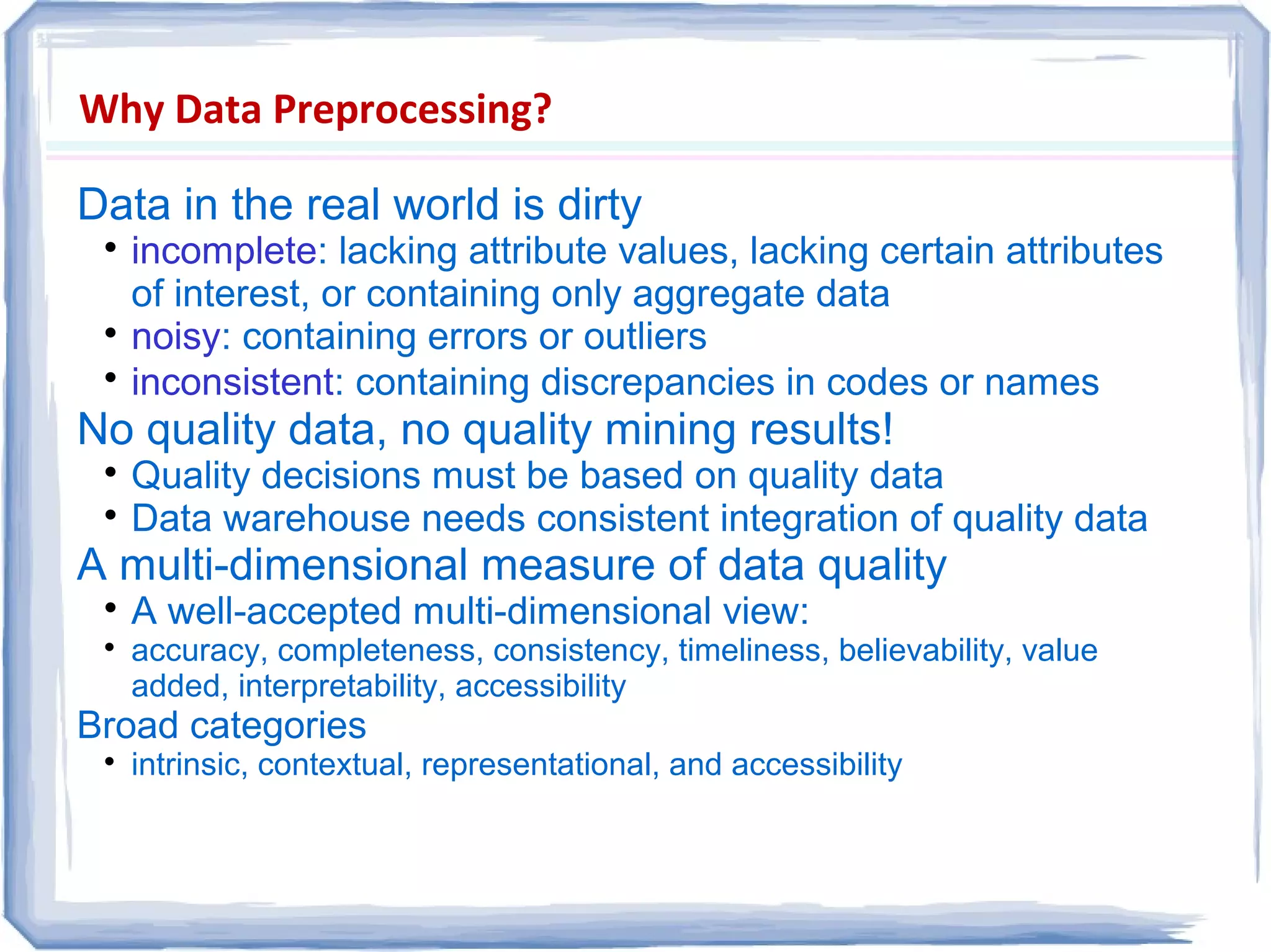
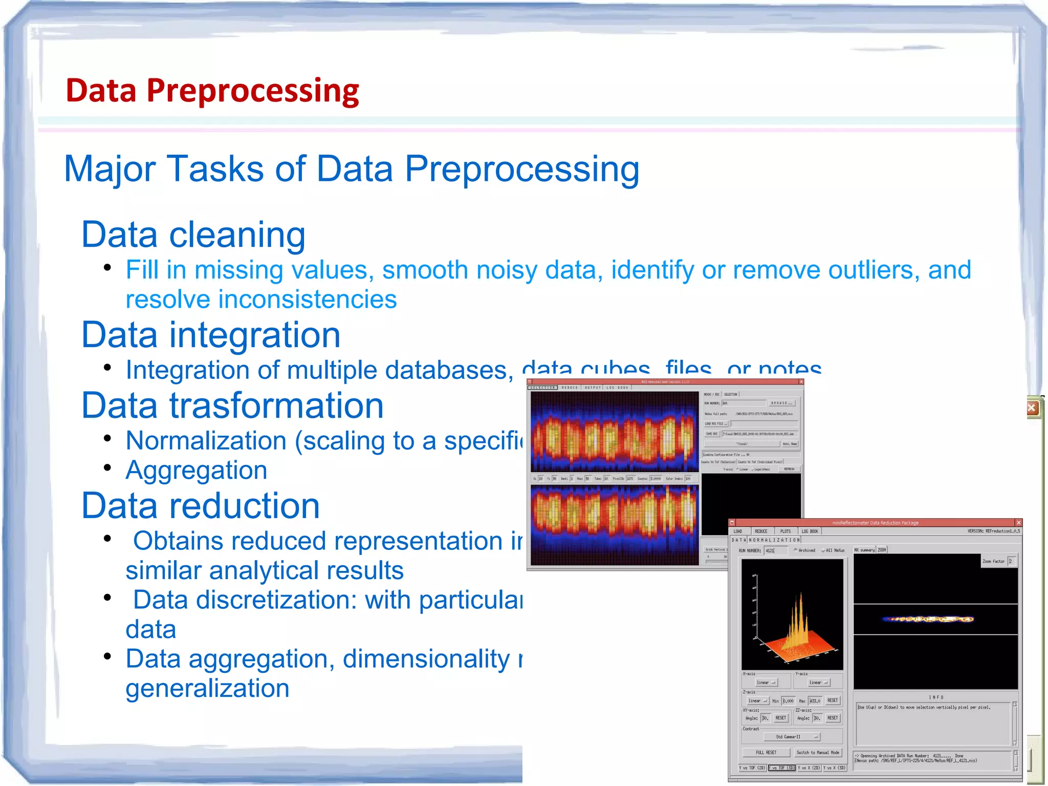
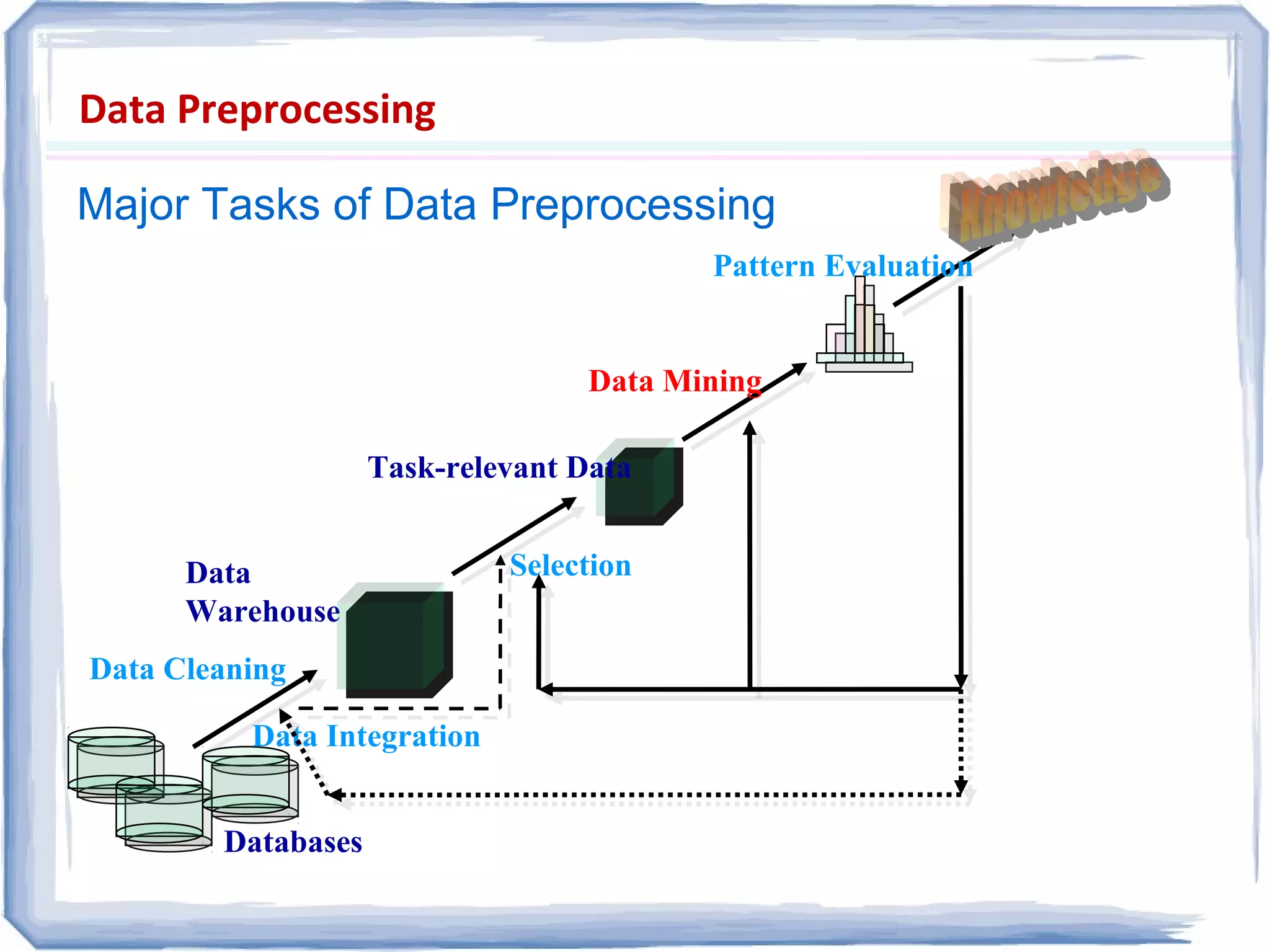
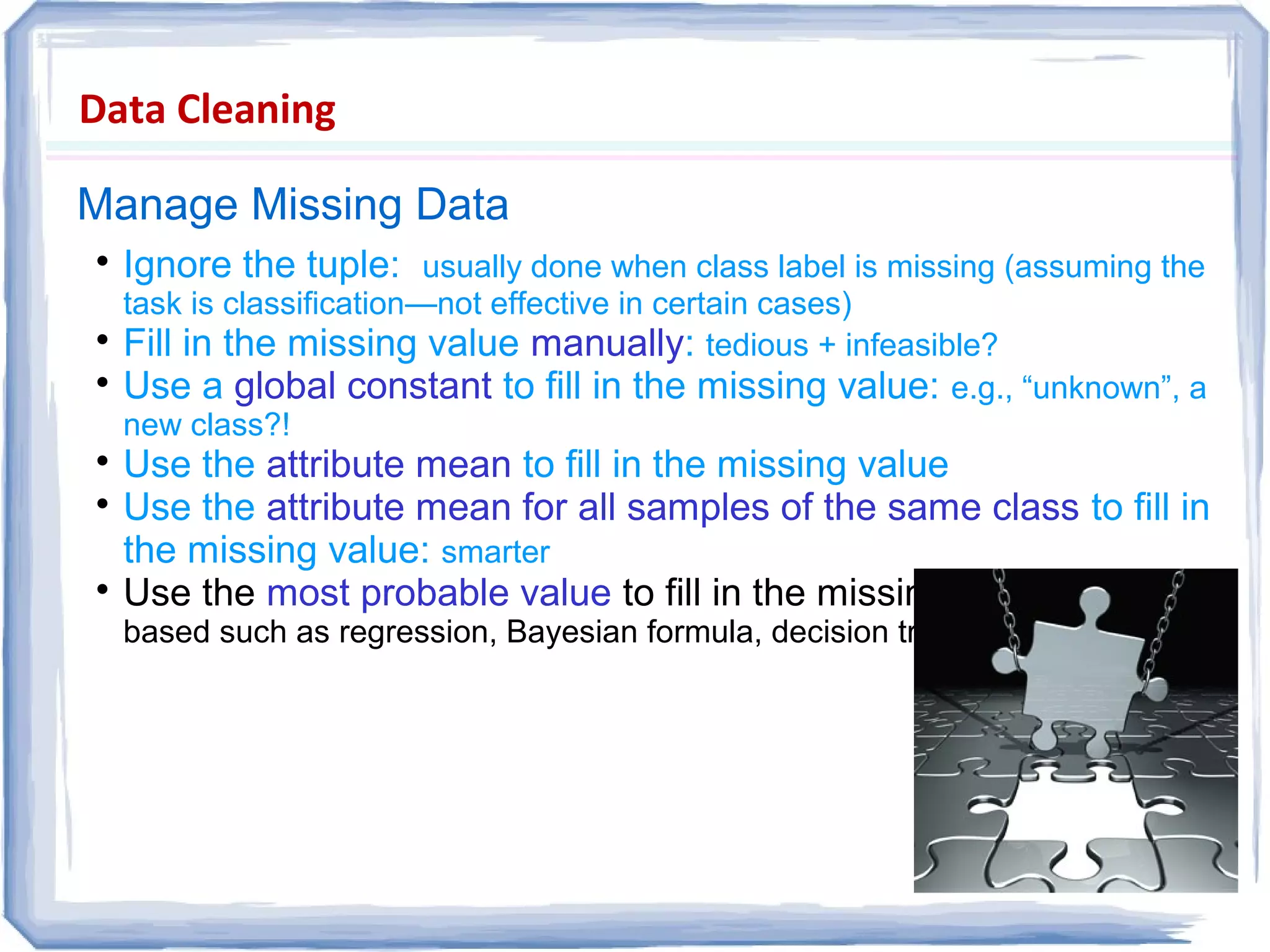
The document presents an overview of data preprocessing, emphasizing its importance for ensuring quality in data mining. It outlines key tasks such as data cleaning, integration, transformation, and reduction, along with methodologies like normalization and aggregation. The document also highlights various data quality dimensions and techniques for managing missing or inconsistent data.

1. A Brief Presentation on Data Mining
Jason Rodrigues
Data Preprocessing

2. • Introduction
• Why data proprocessing?
• Data Cleaning
• Data Integration and
Transformation
• Data Reduction
• Discretization and concept
Heirarchy generation
• Takeaways
Agenda

3. Why Data Preprocessing?
Data in the real world is dirty

incomplete: lacking attribute values, lacking certain attributes
of interest, or containing only aggregate data

noisy: containing errors or outliers

inconsistent: containing discrepancies in codes or names
No quality data, no quality mining results!

Quality decisions must be based on quality data

Data warehouse needs consistent integration of quality data
A multi-dimensional measure of data quality

A well-accepted multi-dimensional view:

accuracy, completeness, consistency, timeliness, believability, value
added, interpretability, accessibility
Broad categories

intrinsic, contextual, representational, and accessibility

4. Data Preprocessing
Major Tasks of Data Preprocessing
Data cleaning

Fill in missing values, smooth noisy data, identify or remove outliers, and
resolve inconsistencies
Data integration

Integration of multiple databases, data cubes, files, or notes
Data trasformation

Normalization (scaling to a specific range)

Aggregation
Data reduction

Obtains reduced representation in volume but produces the same or
similar analytical results

Data discretization: with particular importance, especially for numerical
data

Data aggregation, dimensionality reduction, data compression,
generalization

5. Data Preprocessing
Major Tasks of Data Preprocessing
Data Cleaning
Data Integration
Databases
Data
Warehouse
Task-relevant Data
Selection
Data Mining
Pattern Evaluation

6. Data Cleaning
Tasks of Data Cleaning

Fill in missing values

Identify outliers and smooth noisy data

Correct inconsistent data

7. Data Cleaning
Manage Missing Data

Ignore the tuple: usually done when class label is missing (assuming the
task is classification—not effective in certain cases)

Fill in the missing value manually: tedious + infeasible?

Use a global constant to fill in the missing value: e.g., “unknown”, a
new class?!

Use the attribute mean to fill in the missing value

Use the attribute mean for all samples of the same class to fill in
the missing value: smarter

Use the most probable value to fill in the missing value: inference-
based such as regression, Bayesian formula, decision tree

8. Data Cleaning
Manage Noisy Data
Binning Method:

first sort data and partition into (equi-depth) bins

then one can smooth by bin means, smooth by bin median,
smooth by bin boundaries, etc
Clustering:

detect and remove outliers
Semi Automated

Computer and Manual Intervention
Regression

Use regression functions

9. Data Cleaning
Cluster Analysis

10. Data Cleaning
Regression Analysis
x
y
y = x + 1
X1
Y1
Y1’
•Linear regression (best line to fit
two variables)
•Multiple linear regression (more
than two variables, fit to a
multidimensional surface

11. Data Cleaning
Inconsistant Data

Manual correction using external
references

Semi-automatic using various tools
− To detect violation of known functional
dependencies and data constraints
− To correct redundant data

12. Data integration and transformation
Tasks of Data Integration and transformation

Data integration:
− combines data from multiple sources into a coherent
store

Schema integration
− integrate metadata from different sources
− Entity identification problem: identify real world entities
from multiple data sources, e.g., A.cust-id ≡ B.cust-#

Detecting and resolving data value conflicts
− for the same real world entity, attribute values from
different sources are different
− possible reasons: different representations, different
scales, e.g., metric vs. British units, different currency

13. Manage Data Integration
Data integration and transformation

Redundant data occur often when integrating multiple DBs
− The same attribute may have different names in different databases
− One attribute may be a “derived” attribute in another table, e.g., annual
revenue

Redundant data may be able to be detected by correlational analysis
• Careful integration can help reduce/avoid redundancies and
inconsistencies and improve mining speed and quality
BA
BA
n
BBAA
r
σσ)1(
))((
,
−
−−Σ
=

14. Manage Data Transformation
Data integration and transformation
 Smoothing: remove noise from data (binning, clustering,
regression)
 Aggregation: summarization, data cube construction
 Generalization: concept hierarchy climbing
 Normalization: scaled to fall within a small, specified range
− min-max normalization
− z-score normalization
− normalization by decimal scaling
 Attribute/feature construction
− New attributes constructed from the given ones

15. Manage Data Reduction
Data reduction
Data reduction: reduced representation, while still retaining critical
information

Data cube aggregation

Dimensionality reduction

Data compression

Numerosity reduction

Discretization and concept hierarchy generation

16. Data Cube Aggregation
Data reduction

Multiple levels of aggregation in data cubes
− Further reduce the size of data to deal with

Reference appropriate levels Use the smallest representation capable
to solve the task

17. Data Compression
Data reduction

String compression
− There are extensive theories and well-tuned algorithms
− Typically lossless
− But only limited manipulation is possible without expansion

Audio/video, image compression
− Typically lossy compression, with progressive refinement
− Sometimes small fragments of signal can be reconstructed
without reconstructing the whole

Time sequence is not audio
− Typically short and vary slowly with time
``

18. Decision Tree
Data reduction

19. Similarities and Dissimilarities
Proximity

Proximity is used to refer to Similarity or
Dissimilarity, since proximity between the
object is a function of proximity between
the corresponding attributes of two objects.

Similarity: Numeric measure of the degree
to which the two objects are alike.

Dissimilarity: Numeric measure of the
degree to which the two objects are
different.

20. Dissimilarities between Data Objects?

Similarity
− Numerical measure of how alike two data
objects are.
− Is higher when objects are more alike.
− Often falls in the range [0,1]

Dissimilarity
− Numerical measure of how different are two data
objects
− Lower when objects are more alike
− Minimum dissimilarity is often 0
− Upper limit varies

Proximity refers to a similarity or dissimilarity

21. Euclidean Distance

Euclidean Distance
Where n is the number of dimensions (attributes)
and pk and qk are, respectively, the kth
attributes
(components) or data objects p and q.

Standardization is necessary, if scales differ.
∑
=
−=
n
k
kk qpdist
1
2
)(

22. Euclidean Distance

Euclidean Distance
∑
=
−=
n
k
kk qpdist
1
2
)(
1 2 3 4 5 6 7 8
0
1
2
3
4
5
6
0
5
4
3
Column 2

23. Minkowski Distance
 r = 1. City block (Manhattan, taxicab, L1
norm)
distance.
− A common example of this is the Hamming distance, which is just
the number of bits that are different between two binary vectors

r = 2. Euclidean distance
 r → ∞. “supremum” (Lmax
norm, L∞
norm) distance.
− This is the maximum difference between any component of the
vectors
− Example: L_infinity of (1, 0, 2) and (6, 0, 3) = ??
− Do not confuse r with n, i.e., all these distances are
defined for all numbers of dimensions.

24. Minkowski Distance
point x y
p1 0 2
p2 2 0
p3 3 1
p4 5 1
L1 p1 p2 p3 p4
p1 0 4 4 6
p2 4 0 2 4
p3 4 2 0 2
p4 6 4 2 0
L2 p1 p2 p3 p4
p1 0 2.828 3.162 5.099
p2 2.828 0 1.414 3.162
p3 3.162 1.414 0 2
p4 5.099 3.162 2 0
L∞ p1 p2 p3 p4
p1 0 2 3 5
p2 2 0 1 3
p3 3 1 0 2
p4 5 3 2 0

25. Euclidean Distance Properties
• Distances, such as the Euclidean distance,
have some well known properties.
1. d(x, y) ≥ 0 for all x and y and d(x, y) = 0 only if
x = y. (Positive definiteness)
2. d(x, y) = d(y, x) for all x and q. (Symmetry)
3. d(x, y) ≤ d(x, y) + d(y, z) for all points x, y, and z.
(Triangle Inequality)
where d(x, y) is the distance (dissimilarity) between
points (data objects), x and y.
• A distance that satisfies these properties is a
metric, and a space is called a metric space

26. Non Metric Dissimilarities – Set Differences

non-metric measures are often robust
(resistant to outliers, errors in objects, etc.)
− the symmetry and mainly the triangular inequality
are often violated

cannot be directly
used with MAMs
a
b
a > b + c
c
a
b
a ≠ b

27. Non Metric Dissimilarities – Time

various k-median distances
− measure distance between the two (k-th) most
similar portions in objects

COSIMIR
− back-propagation network with single output
neuron serving as a distance, allows training

Dynamic Time Warping distance
− sequence alignment technique
− minimizes the sum of distances between
sequence elements
 fractional Lp distances
− generalization of Minkowski distances (p<1)
− more robust to extreme differences in coordinates

28. Jaccard Coeffificient

Recall: Jaccard coefficient is a commonly used
measure of overlap of two sets A and B
jaccard(A,B) = |A ∩ B| / |A ∪ B|
jaccard(A,A) = 1
jaccard(A,B) = 0 if A ∩ B = 0

A and B don’t have to be the same size.

JC always assigns a number between 0 and 1.

29. Takeaways
Why Data Preprocessing?
Data Cleaning
Data Integration and Transformation
Data Reduction
Discretization and concept Heirarchy
generation