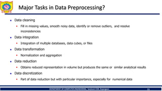
The document is an educational material from Sanjivani College of Engineering discussing data preprocessing techniques in data mining, emphasizing the importance of data quality. It outlines methods for data cleaning, integration, reduction, and transformation to address issues like missing values, noise, and inconsistencies that hinder effective data analysis. Additionally, it highlights the significance of preprocessing in achieving accurate and reliable mining results.

1. Sanjivani Rural Education Society’s
Sanjivani College of Engineering, Kopargaon-423 603
(An Autonomous Institute, Affiliated to Savitribai Phule Pune University, Pune)
NACC ‘A’ Grade Accredited, ISO 9001:2015 Certified
Department of Computer Engineering
(NBA Accredited)
Prof. S.A.Shivarkar
Assistant Professor
Contact No.8275032712
Email- shivarkarsandipcomp@sanjivani.org.in
Subject- Data Mining and Warehousing (CO314)
Unit –II: Data Pre-Processing

2. DEPARTMENT OF COMPUTER ENGINEERING, Sanjivani COE, Kopargaon 2
Data Pre-processing
 Introduction to Data Pre-processing, Data Cleaning: Missing
values,
 Noisy data; Data integration: Correlation analysis; transformation:
 Min-max normalization, z-score normalization and decimal
scaling;
 Data reduction: Data Cube Aggregation, Attribute Subset
Selection,
 Sampling; and Data Discretization: Binning, Histogram Analysis.

3. DEPARTMENT OF COMPUTER ENGINEERING, Sanjivani COE, Kopargaon 3
Data Quality
 Today’s real-world databases are highly susceptible to noisy, missing, and inconsistent
data due to their typically huge size (often several gigabytes or more) and their likely
origin from multiple, heterogenous sources.
 Low-quality data will lead to low-quality mining results.
 “How can the data be preprocessed in order to help improve the quality of the data
and, consequently, of the mining results?
 How can the data be preprocessed so as to improve the efficiency and ease of the
mining process?”

4. DEPARTMENT OF COMPUTER ENGINEERING, Sanjivani COE, Kopargaon 4
Why Data Pre-Prpocessing
 Data in the Real World Is Dirty: Lots of potentially incorrect data, e.g., instrument faulty, human or
computer error, transmission error
 incomplete: lacking attribute values, lacking certain attributes of interest, or containing only aggregate data
e.g., Occupation=“ ” (missing data)
 noisy: containing noise, errors, or outliers
e.g., Salary=“−10” (an error)
 inconsistent: containing discrepancies in codes or names, e.g.,
Age=“42”, Birthday=“03/07/2010”
Was rating “1, 2, 3”, now rating “A, B, C”
discrepancy between duplicate records
 Intentional (e.g., disguised missing data)
Jan. 1 as everyone’s birthday?

5.  Incomplete data may come from
 “Not applicable” data value when collected
 Different considerations between the time when the data was collected and when it is analyzed.
 Human/hardware/software problems
 Noisy data (incorrect values) may come from
 Faulty data collection instruments Human or computer error at data entry Errors in data transmission
 Inconsistent data may come from
 Different data sources
 Functional dependency violation (e.g., modify some linked data)
 Duplicate records also need data cleaning
5
Why Is Data Dirty?

6. 6
Why Is Data Preprocessing Important?
“No quality data, no quality mining results!”
Quality decisions must be based on quality data
•e.g., duplicate or missing data may cause incorrect or even misleading
statistics.
Data warehouse needs consistent integration of quality data Data
extraction, cleaning, and transformation comprises the majority of the
work of building a data warehouse

7. DEPARTMENT OF COMPUTER ENGINEERING, Sanjivani COE, Kopargaon 7
Data Pre-Prepocessing
 There are several data preprocessing techniques:
1. Data cleaning can be applied to remove noise and correct inconsistencies in data. Data
integration merges data from multiple sources into a coherent data store such as a data
warehouse.
2. Data reduction can reduce data size by, for instance, aggregating, eliminating redundant
features, or clustering.
3. Data transformations (e.g., normalization) may be applied, where data are scaled to fall within a
smaller range like 0.0 to 1.0. This can improve the accuracy and efficiency of mining algorithms
involving distance measurements.
 These techniques are not mutually exclusive; they may work together. For example, data
cleaning can involve transformations to correct wrong data, such as by transforming all entries
for a date field to a common format.

8. DEPARTMENT OF COMPUTER ENGINEERING, Sanjivani COE, Kopargaon 8
Data Quality: Why Preprocess the Data?
 Measures for data quality: A multidimensional view
 Accuracy: correct or wrong, accurate or not
 Completeness: not recorded, unavailable, …
 Consistency: some modified but some not, dangling, …
 Timeliness: timely update?
 Believability: how trustable the data are correct?
 Interpretability: how easily the data can be understood?

9. DEPARTMENT OF COMPUTER ENGINEERING, Sanjivani COE, Kopargaon 9
Data Quality: Why Preprocess the Data?
 Measures for data quality: A multidimensional view
 Accuracy: correct or wrong, accurate or not
 Completeness: not recorded, unavailable, …
 Consistency: some modified but some not, dangling, …
 Timeliness: timely update?
 Believability: how trustable the data are correct?
 Interpretability: how easily the data can be understood?

10. DEPARTMENT OF COMPUTER ENGINEERING, Sanjivani COE, Kopargaon 10
Major Tasks in Data Preprocessing?
 Data cleaning
 Fill in missing values, smooth noisy data, identify or remove outliers, and resolve
inconsistencies
 Data integration
 Integration of multiple databases, data cubes, or files
 Data reduction
 Dimensionality reduction
 Numerosity reduction
 Data compression
 Data transformation and data discretization
 Normalization
 Concept hierarchy generation

11. DEPARTMENT OF COMPUTER ENGINEERING, Sanjivani COE, Kopargaon 11
Major Tasks in Data Preprocessing?
 Data cleaning
 Fill in missing values, smooth noisy data, identify or remove outliers, and resolve
inconsistencies
 Data integration
 Integration of multiple databases, data cubes, or files
 Data transformation
 Normalization and aggregation
 Data reduction
 Obtains reduced representation in volume but produces the same or similar analytical results
 Data discretization
 Part of data reduction but with particular importance, especially for numerical data

12. DEPARTMENT OF COMPUTER ENGINEERING, Sanjivani COE, Kopargaon 12
Major Tasks in Data Preprocessing?

13. 13
Incomplete (Missing) Data
 Data is not always available
 E.g., many tuples have no recorded value for several attributes, such as customer income
in sales data
 Missing data may be due to
 equipment malfunction
 inconsistent with other recorded data and thus deleted
 data not entered due to misunderstanding
 certain data may not be considered important at the time of entry
 not register history or changes of the data
 Missing data may need to be inferred

14. 14
How to Handle Missing Data?
 Ignore the tuple: usually done when class label is missing (when doing
classification)—not effective when the % of missing values per attribute varies
considerably
 Fill in the missing value manually: tedious + infeasible?
 Fill in it automatically with
 a global constant : e.g., “unknown”, a new class?!
 the attribute mean
 the attribute mean for all samples belonging to the same class: smarter
 the most probable value: inference-based such as Bayesian formula or decision tree

15. 15
Noisy Data
 Noise: random error or variance in a measured variable
 Incorrect attribute values may be due to
 faulty data collection instruments
 data entry problems
 data transmission problems
 technology limitation
 inconsistency in naming convention
 Other data problems which require data cleaning
 duplicate records
 incomplete data
 inconsistent data

16. 16
How to Handle Noisy Data?
 Binning
 first sort data and partition into (equal-frequency) bins then one can smooth by
bin means, smooth by bin median, smooth by bin boundaries, etc.
 Regression
 smooth by fitting the data into regression functions
 Clustering
 detect and remove outliers
 Combined computer and human inspection
 detect suspicious values and check by human (e.g., deal with possible outliers)

17. 17
Simple Discretization Methods: Binning
 Equal-width (distance) partitioning
 Divides the range into N intervals of equal size: uniform grid
 if A and B are the lowest and highest values of the attribute, the width of intervals will be:
W = (B –A)/N.
 The most straightforward, but outliers may dominate presentation Skewed data is not handled well
 Equal-depth (frequency) partitioning
 Divides the range into N intervals, each containing approximately same number of samples
 Good data scaling
 Managing categorical attributes can be tricky

18. 18
Simple Discretization Methods: Binning cont…
 Equal-width (distance) partitioning
 Sorted data for price (in dollars): 4, 8, 9, 15, 21, 21, 24, 25, 26, 28, 29, 34
 Partition into equal-frequency (equi-depth) bins:
- Bin 1: 4, 8, 9, 15
- Bin 2: 21, 21, 24, 25
- Bin 3: 26, 28, 29, 34
 Smoothing by bin means:
- Bin 1: 9, 9, 9, 9
- Bin 2: 23, 23, 23, 23
- Bin 3: 29, 29, 29, 29
 Smoothing by bin boundaries:
- Bin 1: 4, 4, 4, 15
- Bin 2: 21, 21, 25, 25
- Bin 3: 26, 26, 26, 34

19. Positively and Negatively Correlated Data
Positive Co-relation
Negative Co-relation

20. Not Correlated Data

21. Correlation Analysis (Numerical Data)
 Correlation coefficient (also called ) Pearson’s product moment coefficient)
n σA and σB n σA and σB
  ( A  A')( B  B')
  ( AB )  n AB
rA,B
where n is the number of tuples,
Where
 n is the number of tuples
A’ and B’ are the respective means of A and B
 σAand σB are the respective standard deviation of A and B
Σ(AB) is the sum of the AB cross-product.
If rA,B > 0, A and B are positively correlated (A’s values increase as B’s).
The higher, the stronger correlation.
rA,B = 0: independent;
rA,B < 0: negatively correlated
September 6, 2016 Data Mining: Concepts and Techniques 21

22. Correlation Analysis (Categorical Data)
• Χ2 (chi-square) test
 2
  (Observed  Expected )2
Expected
• The larger the Χ2 value, the more likely the variables are related
• The cells that contribute the most to the Χ2 value are those
whose actual count is very different from the expected count
• Correlation does not imply causality
– # of hospitals and # of car-theft in a city are correlated
– Both are causally linked to the third variable: population

23. Chi-Square Calculation: An Example
Play chess Not play chess Sum (row)
Like science fiction 250(90) 200(360) 450
Not like science fiction 50(210) 1000(840) 1050
Sum(col.) 300 1200 1500
• Χ2 (chi-square) calculation (numbers in parenthesis are expected
counts calculated based on the data distribution in the two
categories)
• It shows that like_science_fiction and play_chess are correlated
• in the group
 507.93
September 6, 2016 Data Mining: Concepts and Techniques 23
 2

(250  90)2

(50  210)2

(200  360)2

(1000 840)2
90 210 360 840

24. Chi-Square Distribution Table
 507.93

25. Cluster Analysis
• It shows that like_science_fiction and play_chess are correlated
in the group
 507.93
25

26. Data integration
 507.93
26
 Data integration:
 Combines data from multiple sources into a coherent store
 Schema integration: e.g., A.cust-id B.cust-#
 Integrate metadata from different sources
 Entity identification problem:
 Identify real world entities from multiple data sources, e.g., Bill Clinton = William Clinton
 Detecting and resolving data value conflicts
 For the same real world entity, attribute values from different sources are different
 Possible reasons: different representations, different scales, e.g., metric vs. British units

27. Handling Redundancy in Data Integration
 Redundant data occur often when integration of multiple databases
Object identification: The same attribute or object may have different names
in different databases
Derivable data: One attribute may be a “derived” attribute in another table, e.g.,
annual revenue
Redundant attributes may be able to be detected by
correlation analysis
 Careful integration of the data from multiple sources may help reduce/avoid
redundancies and inconsistencies

28. Data Transformation
38
 Smoothing: remove noise from data
 Aggregation: summarization, data cube construction Generalization:
concept hierarchy climbing
 Normalization: scaled to fall within a small, specified range
 min-max normalization
 z-score normalization
 normalization by decimal scaling
 Attribute/feature construction
New attributes constructed from the given ones

29. Data Transformation: Normalization
Then $73,000 is mapped to
98,00012,000
(new_ maxA  new_ minA)  new_ minA
v'
 A
– Ex. Let μ = 54,000, σ = 16,000. Then
• Normalization by decimal scaling
v' Where j is the smallest integer such that Max(|ν’|) < 1
16,000
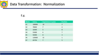
 Min-max normalization: to [new_minA, new_maxA]
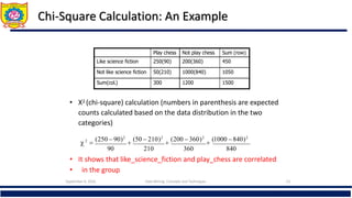
Ex. Let income range $12,000 to $98,000 normalized to [0.0, 1.0]. Then $73,000 is
mapped to
 Z-score normalization (μ: mean, σ: standard deviation):
Ex. Let μ = 54,000, σ = 16,000. Then
 Normalization by decimal scaling
A
A
A
A
A
A
min
new
min
new
max
new
min
max
min
v
v _
)
_
_
(
' 




A
A
v
v




'
j
v
v
10
' Where j is the smallest integer such that Max(|ν’|) < 1
716
.
0
0
)
0
0
.
1
(
000
,
12
000
,
98
000
,
12
600
,
73





225
.
1
000
,
16
000
,
54
600
,
73



30. E.g.
Name Salary Experience in years Position
X1 100000 10 2
X2 78000 7 4
X3 32000 5 8
X4 55000 6 7
X5 92000 8 3
X6 120000 15 1
X7 65750 7 5
Data Transformation: Normalization

31. Example of Decision Tree Induction
Initial attribute set:
{A1, A2, A3, A4, A5, A6}
A4 ?
A1? A6?
Class 1 Class 2 Class 1 Class 2
>
>
Reduced attribute set: {A1, A4,A6}

32. Example of Decision Tree Induction

33.  Divide data into buckets and store
average (sum) for each bucket
 Partitioning rules:
Data Reduction: Histograms Analysis
4
0
3
5
represents)
0
1
0
 Equal-width: equal bucket range Equal-
frequency (or equal-depth)
 V-optimal: with the least histogram variance
(weighted sum of the original values that each
bucket represents)
 MaxDiff: set bucket boundary between each
pair for pairs the β–1 largest differences
1
0
0
0
0
3
3
3
0
0
0
0 5
0
0
0
0 7
0
0
0
0 9
0
0
0
0

34. DEPARTMENT OF COMPUTER ENGINEERING, Sanjivani COE, Kopargaon 34
Reference
 Han, Jiawei Kamber, Micheline Pei and Jian, “Data Mining: Concepts and
Techniques”,Elsevier Publishers, ISBN:9780123814791, 9780123814807.
 https://onlinecourses.nptel.ac.in/noc24_cs22