Control And NonlinearityJeanmichel Coron
download
https://ebookbell.com/product/control-and-nonlinearity-
jeanmichel-coron-2540550
Explore and download more ebooks at ebookbell.com
2.
Here are somerecommended products that we believe you will be
interested in. You can click the link to download.
Diagnosis Of Process Nonlinearities And Valve Stiction Data Driven
Approaches Advances In Industrial Control 1st Edition Ali Ahammad
Shoukat Choudhury
https://ebookbell.com/product/diagnosis-of-process-nonlinearities-and-
valve-stiction-data-driven-approaches-advances-in-industrial-
control-1st-edition-ali-ahammad-shoukat-choudhury-2190250
Stability Of Stationary Sets In Control Systems With Discontinuous
Nonlinearities Series On Stability Vibration And Control Of Systems
Series A Vol 14 Vladimir A Yakubovich
https://ebookbell.com/product/stability-of-stationary-sets-in-control-
systems-with-discontinuous-nonlinearities-series-on-stability-
vibration-and-control-of-systems-series-a-vol-14-vladimir-a-
yakubovich-1320116
Adaptive Backstepping Control Of Uncertain Systems With Actuator
Failures Subsystem Interactions And Nonsmooth Nonlinearities Wang
https://ebookbell.com/product/adaptive-backstepping-control-of-
uncertain-systems-with-actuator-failures-subsystem-interactions-and-
nonsmooth-nonlinearities-wang-7161192
Neurofuzzy Control Of Industrial Systems With Actuator Nonlinearities
F L Lewis
https://ebookbell.com/product/neurofuzzy-control-of-industrial-
systems-with-actuator-nonlinearities-f-l-lewis-1375604
3.
Control And EstimationOf Dynamical Nonlinear And Partial Differential
Equation Systems Theory And Applications Gerasimos Rigatos
https://ebookbell.com/product/control-and-estimation-of-dynamical-
nonlinear-and-partial-differential-equation-systems-theory-and-
applications-gerasimos-rigatos-44888218
Control And Estimation Methods Over Communication Networks Magdi S
Mahmoud
https://ebookbell.com/product/control-and-estimation-methods-over-
communication-networks-magdi-s-mahmoud-46802114
Control And Communication For Demand Response With Thermostatically
Controlled Loads 1st Kai Ma
https://ebookbell.com/product/control-and-communication-for-demand-
response-with-thermostatically-controlled-loads-1st-kai-ma-47434774
Control And Filter Design Of Singlephase Gridconnected Converters 1st
Edition Weimin Wu
https://ebookbell.com/product/control-and-filter-design-of-
singlephase-gridconnected-converters-1st-edition-weimin-wu-47486432
Control And Optimization Based On Network Communication Ximing Sun
https://ebookbell.com/product/control-and-optimization-based-on-
network-communication-ximing-sun-49419994
EDITORIAL COMMITTEE
Jerry L.Bona Peter S. Landweber
Michael G. Eastwood Michael P. Loss
J. T. Stafford, Chair
2000 Mathematics Subject Classification. Primary 93B05, 93B52, 93C10, 93C15,
93C20, 93D15; Secondary 35K50, 35L50, 35L60, 35Q30, 35Q53, 35Q55, 76B75.
For additional information and updates on this book, visit
www.ams.org/bookpages/surv-136
Library of Congress Cataloging-In-Publication Data
Coron. Jean-Michel, 1956-
Control and nonlinearity / Jean-Miche) Coron.
p. cm. - (Mathematical surveys and monographs. ISSN 0076-5376 ; v. 136)
Includes bibliographical references and index.
ISBN-13: 978-0-8218-3668-2 (alk. paper)
ISBN-10: 0-8218-3668-4 (alk. paper)
1. Control theory. 2. Nonlinear control theory. I. Title.
QA402.3.C676 2007
515'.642-dc22 2006048031
Copying and reprinting. Individual readers of this publication, and nonprofit libraries
acting for them, are permitted to make fair use of the material, such as to copy a chapter for use
in teaching or research. Permission is granted to quote brief passages from this publication in
reviews, provided the customary acknowledgment of the source is given.
Republication, systematic copying, or multiple reproduction of any material in this publication
is permitted only under license from the American Mathematical Society. Requests for such
permission should be addressed to the Acquisitions Department, American Mathematical Society,
201 Charles Street, Providence, Rhode Island 02904-2294, USA. Requests can also be made by
e-mail to reprint-permiasionlams.org.
2007 by the American Mathematical Society. All rights reserved.
Printed in the United States of America.
® The paper used in this book is acid-free and falls within the guidelines
established to ensure permanence and durability.
Visit the AMS home page at http://vw.ama.org/
10987654321 1211 10090807
10.
Contents
Preface ix
Part 1.Controllability of linear control systems 1
Chapter 1. Finite-dimensional linear control systems 3
1.1. Definition of controllability 3
1.2. An integral criterion for controllability 4
1.3. Kalman's type conditions for controllability 9
1.4. The Hilbert Uniqueness Method 19
Chapter 2. Linear partial differential equations 23
2.1. Transport equation 24
2.2. Korteweg-de Vries equation 38
2.3. Abstract linear control systems 51
2.4. Wave equation 67
2.5. Heat equation 76
2.6. A one-dimensional Schrodinger equation 95
2.7. Singular optimal control: A linear l-D parabolic-hyperbolic example 99
2.8. Bibliographical complements 118
Part 2. Controllability of nonlinear control systems 121
Chapter 3. Controllability of nonlinear systems in finite dimension 125
3.1. The linear test 126
3.2. Iterated Lie brackets and the Lie algebra rank condition 129
3.3. Controllability of driftless control affine systems 134
3.4. Bad and good iterated Lie brackets 141
3.5. Global results 150
3.6. Bibliographical complements 156
Chapter 4. Linearized control systems and fixed-point methods 159
4.1. The Linear test: The regular case 159
4.2. The linear test: The case of loss of derivatives 165
4.3. Global controllability for perturbations of linear controllable systems 177
Chapter 5. Iterated Lie brackets 181
Chapter 6. Return method 187
6.1. Description of the method 187
6.2. Controllability of the Euler and Navier-Stokes equations 192
11.
vi CONTENTS
6.3. Localcontrollability of a 1-D tank containing a fluid modeled by the
Saint-Venant equations 203
Chapter 7. Quasi-static deformations 223
7.1. Description of the method 223
7.2. Application to a semilinear heat equation 225
Chapter 8. Power series expansion 235
8.1. Description of the method 235
8.2. Application to a Korteweg-de Vries equation 237
Chapter 9. Previous methods applied to a Schrodinger equation 247
9.1. Controllability and uncontrollability results 247
9.2. Sketch of the proof of the controllability in large time 252
9.3. Proof of the nonlocal controllability in small time 263
Part 3. Stabilization 271
Chapter 10. Linear control systems in finite dimension and applications to
nonlinear control systems 275
10.1. Pole-shifting theorem 275
10.2. Direct applications to the stabilization of finite-dimensional control
systems 279
10.3. Gramian and stabilization 282
Chapter 11. Stabilization of nonlinear control systems in finite dimension 287
11.1. Obstructions to stationary feedback stabilization 288
11.2. Time-varying feedback laws 295
11.3. Output feedback stabilization 305
11.4. Discontinuous feedback laws 311
Chapter 12. Feedback design tools 313
12.1. Control Lyapunov function 313
12.2. Damping feedback laws 314
12.3. Homogeneity 328
12.4. Averaging 332
12.5. Backstepping 334
12.6. Forwarding 337
12.7. Transverse functions 340
Chapter 13. Applications to some partial differential equations 347
13.1. Gramian and rapid exponential stabilization 347
13.2. Stabilization of a rotating body-beam without damping 351
13.3. Null asymptotic stabilizability of the 2-D Euler control system 356
13.4. A strict Lyapunov function for boundary control of hyperbolic
systems of conservation laws 361
Appendix A. Elementary results on semigroups of linear operators 373
Appendix B. Degree theory 379
Bibliography 397
Preface
A control systemis a dynamical system on which one can act by using suitable
controls. There are a lot of problems that appear when studying a control system.
But the most common ones are the controllability problem and the stabilization
problem.
The controllability problem is, roughly speaking, the following one. Let us give
two states. Is it possible to move the control system from the first one to the second
one? We study this problem in Part 1 and in Part 2. Part 1 studies the control-
lability of linear control systems, where the situation is rather well understood,
even if there are still quite challenging open problems in the case of linear partial
differential control systems. In Part 2 we are concerned with the controllability
of nonlinear control systems. We start with the case of finite-dimensional control
systems, a case where quite powerful geometrical tools are known. The case of
nonlinear partial differential equations is much more complicated to handle. We
present various methods to treat this case as well as many applications of these
methods. We emphasize control systems for which the nonlinearity plays a crucial
role, in particular, for which it is the nonlinearity that gives the controllability or
prevents achieving some specific interesting motions.
The stabilization problem is the following one. We have an equilibrium which
is unstable without the use of the control. Let us give a concrete example. One
has a stick that is placed vertically on one of his fingers. In principle, if the stick is
exactly vertical with a speed exactly equal to 0, it should remain vertical. But, due
to various small errors (the stick is not exactly vertical, for example), in practice,
the stick falls down. In order to avoid this, one moves the finger in a suitable
way, depending on the position and speed of the stick; we use a "feedback law"
(or "closed-loop control") which stabilizes the equilibrium. The problem of the
stabilization is the existence and construction of such stabilizing feedback laws
for a given control system. We study it in Part 3, both for finite-dimensional
control systems and for systems modeled by partial differential equations. Again
we emphasize the case where the nonlinear terms play a crucial role.
Let us now be more precise on the contents of the different parts of this book.
Part 1: Controllability of linear control systems
This first part is devoted to the controllability of linear control systems. It has two
chapters: The first one deals with finite-dimensional control systems, the second
one deals with infinite-dimensional control systems modeled by partial differential
equations.
Let us detail the contents of these two chapters.
ix
15.
x PREFACE
Chapter 1.This chapter focuses on the controllability of linear finite-dimensional
control systems. We first give an integral necessary and sufficient condition for
a linear time-varying finite-dimensional control system to be controllable. For a
special quadratic cost, it leads to the optimal control. We give some examples of
applications.
These examples show that the use of this necessary and sufficient condition can
lead to computations which are somewhat complicated even for very simple control
systems. In particular, it requires integrating linear differential equations. We
present the famous Kalman rank condition for the controllability of linear time-
invariant finite-dimensional control systems. This new condition, which is also
necessary and sufficient for controllability, is purely algebraic: it does not require
integrations of linear differential equations. We turn then to the case of linear time-
varying finite-dimensional control systems. For these systems we give a sufficient
condition for controllability, which turns out to be also necessary for analytic control
systems. This condition only requires computing derivatives; again no integrations
are needed.
We describe, in the framework of linear time-varying finite-dimensional control
systems, the Hilbert Uniqueness Method (HUM), due to Jacques-Louis Lions. This
method is quite useful in infinite dimension for finding numerically optimal controls
for linear control systems.
Chapter 2. The subject of this chapter is the controllability of some classical linear
partial differential equations. For the reader who is familiar with this subject, a
large part of this chapter can be omitted; most of the methods detailed here are
very well known. One can find much more advanced material in some references
given throughout this chapter. We study a transport equation, a Korteweg-de Vries
equation, a heat equation, a wave equation and a Schrodinger equation.
We prove the well-posedness of the Cauchy problem associated to these equa-
tions. The controllability of these equations is studied by means of various methods:
explicit methods, extension method, moments theory, flatness, Hilbert Uniqueness
Method, duality between controllability and observability. This duality shows that
the controllability can be reduced to an observability inequality. We show how
to prove this inequality by means of the multiplier method or Carleman inequal-
ities. We also present a classical abstract setting which allows us to treat the
well-posedness and the controllability of many partial differential equations in the
same framework.
Part 2: Controllability of nonlinear control systems
This second part deals with the controllability of nonlinear control systems.
We start with the case of nonlinear finite-dimensional control systems. We
recall the linear test and explain some geometrical methods relying on iterated Lie
brackets when this test fails.
Next we consider nonlinear partial differential equations. For these infinite-
dimensional control systems, we begin with the case where the linearized control
system is controllable. Then we get local controllability results and even global
controllability results if the nonlinearity is not too big. The case where the linearized
control system is not controllable is more difficult to handle. In particular, the
tool of iterated Lie brackets, which is quite useful for treating this case in finite
16.
PREFACE xi
dimension, turnsout to be useless for many interesting infinite-dimensional control
systems. We present three methods to treat some of these systems, namely the
return method, quasi-static deformations and power series expansions. On various
examples, we show how these three methods can be used.
Let us give more details on the contents of the seven chapters of Part 2.
Chapter 3. In this chapter we study the local controllability of finite-dimensional
nonlinear control systems around a given equilibrium. One does not know any in-
teresting necessary and sufficient condition for small-time local controllability, even
for analytic control systems. However, one knows powerful necessary conditions
and powerful sufficient conditions.
We recall the classical "linear test": If the linearized control system at the
equilibrium is controllable, then the nonlinear control system is locally controllable
at this equilibrium.
When the linearized control system is not controllable, the situation is much
more complicated. We recall the Lie algebra condition, a necessary condition for
local controllability of (analytic) control systems. It relies on iterated Lie brackets.
We explain why iterated Lie brackets are natural for the problem of controllability.
We study in detail the case of the driftless control systems. For these systems,
the above Lie algebra rank condition turns out to be sufficient, even for global
controllability.
Among the iterated Lie brackets, we describe some of them which are "good"
and give the small-time local controllability, and some of them which are "bad"
and lead to obstructions to small-time local controllability.
Chapter 4. In this chapter, we first consider the problem of the controllability
around an equilibrium of a nonlinear partial differential equation such that the
linearized control system around the equilibrium is controllable. In finite dimension,
we have already seen that, in such a situation, the nonlinear control system is
locally controllable around the equilibrium. Of course in infinite dimension one
expects that a similar result holds. We prove that this is indeed the case for
various equations: A nonlinear Korteweg-de Vries equation, a nonlinear hyperbolic
equation and a nonlinear Schrodinger equation. For the first equation, one uses
a natural fixed-point method. For the two other equations, the situation is more
involved due to a problem of loss of derivatives. For the hyperbolic equation, one
uses, to take care of this problem, an ad-hoc fixed-point method, which is specific
to hyperbolic systems. For the case of the Schrodinger equation, this problem is
overcome by the use of a Nash-Moser method.
Sometimes these methods, which lead to local controllability results, can be
adapted to give a global controllability result if the nonlinearity is not too big at
infinity. We present an example for a nonlinear one-dimensional wave equation.
Chapter 5. We present an application of the use of iterated Lie brackets for a
nonlinear partial differential equation (a nonlinear Schrodinger equation). We also
explain why iterated Lie brackets are less powerful in infinite dimension than in
finite dimension.
17.
xii PREFACE
Chapter 6.This chapter deals with the return method. The idea of the return
method goes as follows: If one can find a trajectory of the nonlinear control system
such that:
- it starts and ends at the equilibrium,
- the linearized control system around this trajectory is controllable,
then, in general, the implicit function theorem implies that one can go from every
state close to the equilibrium to every other state close to the equilibrium. In
Chapter 6, we sketch some results in flow control which have been obtained by this
method, namely:
- global controllability results for the Euler equations of incompressible fluids,
- global controllability results for the Navier-Stokes equations of incompress-
ible fluids,
- local controllability of a 1-D tank containing a fluid modeled by the shallow
water equations.
Chapter 7. This chapter develops the quasi-static deformation method, which
allows one to prove in some cases that one can move from a given equilibrium to
another given equilibrium if these two equilibria are connected in the set of equi-
libria. The idea is just to move very slowly the control (quasi-static deformation)
so that at each time the state is close to the curve of equilibria connecting the two
given equilibria. If some of these equilibria are unstable, one also uses suitable feed-
back laws in order to stabilize them; without these feedback laws the quasi-static
deformation method would not work. We present an application to a semilinear
heat equation.
Chapter 8. This chapter is devoted to the power series expansion method: One
makes some power series expansion in order to decide whether the nonlinearity
allows us to move in every (oriented) direction which is not controllable for the
linearized control system around the equilibrium. We present an application to a
nonlinear Korteweg-de Vries equation.
Chapter 9. The previous three methods (return, quasi-static deformations, power
series expansion) can be used together. We present in this chapter an example for
a nonlinear Schrodinger control equation.
Part 3: Stabilization
The two previous parts were devoted to the controllability problem, which asks if
one can move from a first given state to a second given state. The control that
one gets is an open-loop control: it depends on time and on the two given states,
but it does not depend on the state during the evolution of the control system.
In many practical situations one prefers closed-loop controls, i.e., controls which
do not depend on the initial state but depend, at time t, on the state x at this
time. One requires that these closed-loop controls (asymptotically) stabilize the
point one wants to reach. Usually such closed-loop controls (or feedback laws) have
the advantage of being be more robust to disturbances (recall the experiment of
the stick on the finger). The main issue discussed in this part is the problem of
deciding whether a controllable system can be (asymptotically) stabilized.
18.
PREFACE xiii
This partis divided into four chapters: Chapter 10, Chapter 11, Chapter 12
and Chapter 13, which we now briefly describe.
Chapter 10. This chapter is mainly concerned with the stabilization of finite-
dimensional linear control systems. We first start by recalling the classical pole-
shifting theorem. A consequence of this theorem is that every controllable linear
system can be stabilized by means of linear feedback laws. This implies that, if
the linearized control system at an equilibrium of a nonlinear control system is
controllable, then this equilibrium can be stabilized by smooth feedback laws.
Chapter 11. This chapter discusses the stabilization of finite-dimensional non-
linear control systems, mainly in the case where the nonlinearity plays a key role.
In particular, it deals with the case where the linearized control system around
the equilibrium that one wants to stabilize is no longer controllable. Then there
are obstructions to stabilizability by smooth feedback laws even for controllable
systems. We recall some of these obstructions. There are two ways to enlarge the
class of feedback laws in order to recover stabilizability properties. The first one is
the use of discontinuous feedback laws. The second one is the use of time-varying
feedback laws. We give only comments and references on the first method, but we
give details on the second one. We also show the interest of time-varying feedback
laws for output stabilization: In this case the feedback laws depend only on the
output, which is only part of the state.
Chapter 12. In this chapter, we present important tools for constructing explicit
stabilizing feedback laws, namely:
1. control Lyapunov function,
2. damping,
3. homogeneity.
4. averaging,
5. backstepping,
6. forwarding,
7. transverse functions.
These methods are illustrated on various control systems, in particular, the stabi-
lization of the attitude of a rigid spacecraft.
Chapter 13. In this chapter, we give examples of how some tools introduced for
the stabilization of finite-dimensional control systems can be used to stabilize some
partial differential equations. We treat the following four examples:
1. rapid exponential stabilization by means of Gramians for linear time-rever-
sible partial differential equations,
2. stabilization of a rotating body-beam without damping,
3. stabilization of the Euler equations of incompressible fluids,
4. stabilization of hyperbolic systems.
19.
xiv PREFACE
Appendices
This bookhas two appendices. In the first one (Appendix A), we recall some classi-
cal results on semigroups generated by linear operators and classical applications to
evolution equations. We omit the proofs but we give precise references where they
can be found. In the second appendix (Appendix B), we construct the degree of a
map and prove the properties of the degree we use in this book. As an application
of the degree, we also prove the Brouwer and Schauder fixed-point theorems which
are also used in this book.
Acknowledgments. I thank the Rutgers University Mathematics Depart-
ment, especially Eduardo Sontag and Hector Sussmann, for inviting me to give the
2003 Dean Jacqueline B. Lewis Memorial Lectures. This book arose from these
lectures. I am grateful to the Institute Universitaire de France for providing ideal
working conditions for writing this book.
It is a pleasure to thank Azgal Abichou, Claude Bardos, Henry Hermes, Vil-
mos Komornik, Marius Tucsnak, and Jose Urquiza, for useful discussions. I am
also especially indebted to Karine Beauchard, Eduardo Cerpa, Yacine Chitour,
Emmanuelle Crepeau, Olivier Glass, Sergio Guerrero, Thierry Horsin, Rhouma
Mlayeh, Christophe Prieur, Lionel Rosier, Emmanuel Trelat, and Claire Voisin
who recommended many modifications and corrections. I also thank Claire Voisin
for important suggestions and for her constant encouragement.
It is also a pleasure to thank my former colleagues at the Centre Automatique et
Systemes, Brigitte d'Andrea^Novel, Frangois Chaplais, Michel Fliess, Yves Lenoir,
Jean Levine, Philippe Martin, Nicolas Petit, Laurent Praly and Pierre Rouchon,
for convincing me to work in control theory.
Jean-Michel Coron
October, 2006
This first partis devoted to the controllability of linear control systems. It has
two chapters: The first one deals with finite-dimensional control systems, the second
one deals with infinite-dimensional control systems modeled by partial differential
equations.
Let us detail the contents of these two chapters.
Chapter 1. This chapter focuses on the controllability of linear finite-dimensional
control systems. We first give an integral necessary and sufficient condition (The-
orem 1.11 on page 6) for a linear time-varying finite-dimensional control system
to be controllable. For a special quadratic cost, it leads to the optimal control
(Proposition 1.13 on page 8). We give examples of applications.
These examples show that the use of this necessary and sufficient condition
can lead to computations which are somewhat complicated even for very simple
control systems. In particular, it requires integrating linear differential equations.
In Section 1.3 we first give the famous Kalman rank condition (Theorem 1.16 on
page 9) for the controllability of linear time-invariant finite-dimensional control sys-
tems. This new condition, which is also necessary and sufficient for controllability,
is purely algebraic; it does not require integrations of linear differential equations.
We turn then to the case of linear time-varying finite-dimensional control systems.
For these systems we give a sufficient condition for controllability (Theorem 1.18
on page 11), which turns out to be also necessary for analytic control systems. This
condition only requires computing derivatives. Again no integrations are needed.
In Section 1.4, we describe, in the framework of linear time-varying finite-
dimensional control systems, the Hilbert Uniqueness Method, due to Jacques-Louis
Lions. This method is quite useful in infinite dimension to find numerically optimal
controls for linear control systems.
Chapter 2. The subject of this chapter is the controllability of some classical
partial differential equations. For the reader who is familiar with this subject, a
large part of this chapter can be omitted; most of the methods detailed here are
very well known. The linear partial differential equations which are treated are the
following:
1. a transport equation (Section 2.1),
2. a Korteweg-de Vries equation (Section 2.2),
3. a one-dimensional wave equation (Section 2.4),
4. a heat equation (Section 2.5),
5. a one-dimensional Schrodinger equation (Section 2.6),
6. a family of one-dimensional heat equations depending on a small parameter
(Section 2.7).
For these equations, after proving the well-posedness of the Cauchy problem, we
study their controllability by means of various methods (explicit method, extension
method, duality between controllability and observability, observability inequalities,
multiplier method, Carleman inequalities, moment theory, Laplace transform and
harmonic analysis ...). We also present in Section 2.3 a classical abstract setting
which allows us to treat the well-posedness and the controllability of many partial
differential equations in the same framework.
22.
CHAPTER 1
Finite-dimensional linearcontrol systems
This chapter focuses on the controllability of linear finite-dimensional control
systems. It is organized as follows.
- In Section 1.2 we give an integral necessary and sufficient condition (The-
orem 1.11 on page 6) for a linear time-varying finite-dimensional control
system to be controllable. For a special quadratic cost, it leads to the opti-
mal control (Proposition 1.13 on page 8). We give examples of applications.
- These examples show that the use of this necessary and sufficient, condi-
tion can lead to computations which are somewhat complicated even for
very simple control systems. In particular, it requires integrating linear
differential equations. In Section 1.3 we first give the famous Kalman rank
condition (Theorem 1.16 on page 9) for the controllability of linear time-
invariant finite-dimensional control systems. This new condition, which is
also necessary and sufficient for controllability, is purely algebraic; it does
not require integrations of linear differential equations. We turn then to
the case of linear time-varying finite-dimensional control systems. For these
systems we give a sufficient condition for controllability (Theorem 1.18 on
page 11), which turns out to be also necessary for analytic control systems.
This condition only requires computing derivatives. Again no integrations
are needed. We give two proofs of Theorem 1.18. The first one is the
classical proof. The second one is new.
- In Section 1.4, we describe, in the framework of linear time-varying finite-
dimensional control systems, the Hilbert Uniqueness Method (HUM), due
to Jacques-Louis Lions. This method, which in finite dimension is strongly
related to the integral necessary and sufficient condition of controllability
given in Section 1.2, is quite useful in infinite dimension to find numerically
optimal controls for linear control systems.
1.1. Definition of controllability
Let us start with some notations. For k E N {0}, Rk denotes the set of
k-dimensional real column vector. For k E N {O} and I E N (0), we denote
by £(R'; R') the set of linear maps from Rk into R. We often identify, in the
usual way, £(R';R') with the set, denoted Mk,i(R), of k x I matrices with real
coefficients. We denote by Mk,i(C) the set of k x I matrices with complex co-
efficients. Throughout this chapter, To, Ti denote two real numbers such that
To < T1, A : (TO,T1) -* C(R";R") denotes an element of L' ((TO, Tj);,C(Rn; R"))
and B : (TO,Ti) L(Rm;R") denotes an element of L°°((To,T1);L(Rm;R")). We
consider the time-varying linear control system
(1.1) i=A(t)x+B(t)u, t E [To, T1],
3
23.
4 1. FINITE-DIMENSIONALLINEAR CONTROL SYSTEMS
where, at time t E [TO,TI], the state is x(t) E R" and the control is u(t) E R'", and
dx/dt.
We first define the solution of the Cauchy problem
(1.2) i = A(t)x + B(t)u(t), x(To) = x°,
for given u in LI ((T°, T1); R') and given x° in R".
DEFINITION 1.1. Let b E LI ((To, TI); R"). A map x : (TO, T11 - R' is a solution
of
(1.3) i = A(t)x + b(t), t E (To, TI ),
if x E C°([To,TI];R") and satisfies
x(t2) = x(tI) +
J
12
(A(t)x(t) + b(t))dt, V(tl, t2) E [T0, T1]2.
In particular, for xo E R", a solution to the Cauchy problem
(1.4) i = A(t)x + b(t), t E (To, Ti), x(To) = x°
is a function x E C°([To,T1];R") such that
x(r) = x° + J (A(t)x(t) + b(t))dt, Vr E [To, T1].
To
It is well known that, for every b E L' ((To, TI ); R") and for every x° E R", the
Cauchy problem (1.4) has a unique solution.
Let us now define the controllability of system (1.1). (This concept goes back
to Rudolph Kalman [263, 264].)
DEFINITION 1.2. The linear time-varying control system (1.1) is controllable
if, for every (x°,x1) E R" x R", there exists u E L°°((To,T1);Rm) such that the
solution x E C°([To,TI]; R") of the Cauchy problem (1.2) satisfies x(T1) = xI.
REMARK 1.3. One could replace in this definition u E L°O((ToiT1);Rm) by
u E L2 ((To, T1); R'") or by u E L' ((To, T1); R'"). It follows from the proof of Theo-
rem 1.11 on page 6 that these changes of spaces do not lead to different controllable
systems. We have chosen to consider u E L°°((To,T1);Rm) since this is the natu-
ral space for general nonlinear control system (see, in particular, Definition 3.2 on
page 125).
1.2. An integral criterion for controllability
We are now going to give a necessary and sufficient condition for the control-
lability of system (1.1) in terms of the resolvent of the time-varying linear system
i = A(t)x. This condition is due to Rudolph Kalman, Yu-Chi Ho and Kumpati
Narendra (265, Theorem 5]. Let us first recall the definition of the resolvent of the
time-varying linear system i = A(t)x.
DEFINITION 1.4. The resolvent R of the time-varying linear system i = A(t)x
is the map
R : [To, T,]2 C(R"; R")
(tt,t2) '-' R(t1,t2)
24.
1.2. AN INTEGRALCRITERION FOR CONTROLLABILITY 5
such that, for every t2 E [To, T1], the map R(-, t2) : [TO,T1] - G(R";R"), tj
R(t1, t2), is the solution of the Cauchy problem
(1.5) M = A(t)M, M(t2) = Id",
where Id,, denotes the identity map of R".
One has the following classical properties of the resolvent.
PROPOSITION 1.5. The resolvent R is such that
(1.6) R E Co([To,Ti]2;.C(R";R")),
(1.7) R(t1, t1) = Idn, Vt1 E [To,T1],
(1.8) R(t1, t2) R(t2, t3) = R(t1, t3), V(t 1, t2, t3) E [To, T1]3.
In particular,
(1.9) R(t1, t2)R(t2, t1) = Idn, d(tl, t2) E [To, T1]2.
Moreover, if A E C°([To,Tl];G(R";R")), then R E C1([To,Tl]2;I(R";R")) and
one has
(1.10) (t, r) = A(t)R(t,-r), d(t,T) E [TO,T1]2,
(1.11) 2(t,r) _ -R(t,T)A(T),V(t,T) C- [TO, T11'.
REMARK 1.6. Equality (1.10) follows directly from the definition of the re-
solvent. Equality (1.11) can be obtained from (1.10) by differentiating (1.9) with
respect to t2.
EXERCISE 1.7. Let us define A by
A(t) = (1 tl)
Compute the resolvent of i = A(t)x.
Answer. Let x1 and X2 be the two components of x in the canonical basis of
R2. Let z = x1 + ix2 E C. One gets
z = (t + i)z,
which leads to
(1.12) z(t1) = z(t2) exp (2 - 2 + it1 - it2) .
From (1.12), one gets
cos(tl - t2)
R(tl, t2) =
sin(tl - t2)
EXERCISE 1.8. Let A be in C1([To,TI];G(R",R")).
1. For k E N, compute the derivative of the map
[To,T1] C(R",R")
t ,.. A(t)k.
25.
6 1. FINITE-DIMENSIONALLINEAR CONTROL SYSTEMS
2. Let us assume that
A(t)A(r) = A(r)A(t), V(t, T) E [TO,T1]2.
Show that
(1.13) R(t1, t2) = exp Ut2
A(t)dt)
, V(t1, t2) E [To, Ti]2.
e
3. Give an example of A such that (1.13) does not hold.
Answer. Take n = 2 and
/
A(t) :=
0 t
I 0 1 .
One gets, for every (t1it2) E [To,T1]2,
_ (1 (t1 - 1)etl-t3 - t2 + 1)
R(t1, t2) - 0 eti-h
t
t
t, 2 (et, -tz - 1)
1 +
1
exp
(112
A(t)dt) 2
0 etc-ta
Of course, the main property of the resolvent is the fact that it gives the solution
of the Cauchy problem (1.4). Indeed, one has the following classical proposition.
PROPOSITION 1.9. The solution of the Cauchy problem (1.4) satisfies
(1.14) x(t1) = R(t1,to)x(to)+ f
tl
R(t1,r)b(r)dr, V(to,t1) E [To,T1]2
to
In particular,
R(t, r)b(r)dr, Vt E [To,T1].
(1.15) x(t) = R(t,To)x° +J
o
Equality (1.14) is known as Duhamel's principle.
Let us now define the controllability Gramian of the control system i = A(t)x+
B(t)u.
DEFINITION 1.10. The controllability Gramian of the control system
i = A(t)x + B(t)u
is the symmetric n x n-matrix
T
(1.16) 4r:=
J
R(TI, r)B(r)B(r)t`R(T1i r)t`dr.
To
In (1.16) and throughout the whole book, for a matrix M or a linear map M
from R' into RI, Mtr denotes the transpose of M.
Our first condition for the controllability of i = A(t)x + B(t)u is given in
the following theorem [265, Theorem 5] due to Rudolph Kalman, Yu-Chi Ho and
Kumpati Narendra.
THEOREM 1.11. The linear time varying control system i = A(t)x + B(t)u is
controllable if and only if its controllability Gramian is invertible.
26.
1.2. AN INTEGRALCRITERION FOR CONTROLLABILITY 7
REMARK 1.12. Note that, for every x E R",
T,
xtr& = f !B(T)tr R(Ti,T)trxI2dr.
To
Hence the controllability Gramian (E is a nonnegative symmetric matrix. In partic-
ular, C is invertible if and only if there exists c > 0 such that
(1.17) xt'Cx > CIx12, Vx E R.
Proof of Theorem 1.11. We first assume that it is invertible and prove that
i = A(t)x+B(t)u is controllable. Let x° and x1 be in R n. Let u E LOO ((To, TI); Rm)
be defined by
(1.18) u(r) := B(T)trR(Ti,r)`(E-1(x1
- R(Ti,To)x°), T E (TO,T1).
(In (1.18) and in the following, the notation "r E (To,T1)" stands for "for almost
every r E (To, T1)" or in the distribution sense in D'(To, T1), depending on the
context.) Let x E CO ([To, TI ]; R") be the solution of the Cauchy problem
(1.19) x = A(t)-;- + B(t)u(t), x(To) = x0.
Then, by Proposition 1.9,
D(TI) = R(Ti,To)xo
+ f o' R(Ti,T)B(T)B(T)t`R(Ti,T)t`4E-I(x' - R(T1,To)x°)dr
= R(Ti,To)x° +x1 - R(Ti,To)x°
= x1
Hence i = A(t)x + B(t)u is controllable.
Let us now assume that C is not invertible. Then there exists y E R" {0} such
that ty = 0. In particular, ytrlry = 0, that is,
T1
(1.20)
1
ytrR(TT,T)B(T)B(T)t`R(T1,T)trydT = 0.
To
But the left hand side of (1.20) is equal to
T
ITo
1
I B(T)t`R(Ti,T)%ryj2dT.
Hence (1.20) implies that
(1.21) yt`R(TI,T)B(T) = 0,T E (To, T1)
Now let u E L1((To,T1); Rm) and x E C°([To,T1]; R") be the solution of the Cauchy
problem
i = A(t)x + B(t)u(t), x(To) = 0.
Then, by Proposition 1.9 on the previous page,
Tt
x(T1) =
J
R(TI,T)B(T)u(T)dr.
To
In particular, by (1.21),
(1.22) yt`x(Ti) = 0.
Since y E R" {0}, there exists x1 E R" such that ytrxl # 0 (for example x1 := y).
It follows from (1.22) that, whatever u is, x(T1) # x1. This concludes the proof of
Theorem 1.11.
27.
8 1. FINITE-DIMENSIONALLINEAR CONTROL SYSTEMS
Let us point out that the control ii defined by (1.18) has the quite interesting
property given in the following proposition, also due to Rudolph Kalman, Yu-Chi
Ho and Kumpati Narendra [265, Theorem 8].
PROPOSITION 1.13. Let (x°,x') E R' x R' and let u E L2((To,TI);Rm) be
such that the solution of the Cauchy problem
(1.23) i = A(t)x + B(t)u, x(To) = x°,
satisfies
Then
x(Ti) = x'.
1T1
T
lu(t)I2dt <
J
1 Iu(t)I2dt
To To
with equality (if and) only if
u(t) = u(t) for almost every t E (To,TI).
Proof of Proposition 1.13. Let v:= u-u. Then, 2 and x being the solutions
of the Cauchy problems (1.19) and (1.23), respectively, one has
f p' R(Ti, t)B(t)v(t)dt = fo' R(Ti, t)B(t)u(t)dt - fa' R(Ti, t)B(t)u(t)dt
= (x(Ti) - R(Ti,To)x(To))
- (i(T1) - R(Ti,To)x(To))
Hence
(1.24)
One has
(1.25)
T
TO
1
R(Ti, t)B(t)v(t)dt =
(x'
- R(Ti,To)x°) - (x' - R(Ti,To)x°) = 0.
T
1Ltr(T)v(T)dT.
I 1 Iu(T)I2dT =
J
T 1 I a(T)I2dT + Iv(T)I2dT + 2
J
'
o To To To
From (1.18) (note also that qtr = e:),
TAI
iitr(T)v(T)dT = (x' - fT.
T3 R(Ti,T)B(r)v(T)dr,
T.
which, together with (1.24), gives
f T1
(1.26) utr(T)v(T)dT = 0.
o
Proposition 1.13 then follows from (1.25) and (1.26).
EXERCISE 1.14. Let us consider the control system
(1.27) it = u, i2 = x1 + tu,
where the control is u E R and the state is x := (x1ix2)Ir E R2. Let T > 0. We
take To := 0 and TI := T. Compute e:. Check that the control system (1.27) is not
controllable.
Answer. One finds
T T2
= 7,2 T3 ,
which is a matrix of rank 1.
28.
1.3. KALMAN'S TYPECONDITIONS FOR CONTROLLABILITY 9
EXERCISE 1.15. Let us consider the control system
(1.28) i1 = x2, i2 = U,
where the control is u E R and the state is x := (x1ix2)t E R2. Let T > 0.
Compute the u E L'(0, T) which minimizes f0 Ju(r)12dr under the constraint that
the solution x of (1.28) such that x(0) _ (-1,0)tr satisfies x(T) = (0,0)Ir
Answer. Let To = 0, T1 = T, xo = (-1 0)t' and x1 = (0, 0)tr. One gets
R(Tj,r) =
1 T-7-
0 1 tlr E [To,T,
T2 T2
1
12
C
1 -T/
= T7 2 3 _T T ,
2 T T 2 s
which lead to
12 T 12 /t2 T 12 ft3 T
u(t)7,3t- 2 I,xs(t)7,31 2 - 2t1x1(t)=-1-7,31 6 - 4t21.
1.3. Kalman's type conditions for controllability
The necessary and sufficient condition for controllability given in Theorem 1.11
on page 6 requires computing the matrix Ir, which might be quite difficult (and even
impossible) in many cases, even for simple linear control systems. In this section
we give a new criterion for controllability which is much simpler to check.
For simplicity, we start with the case of a time invariant system, that is, the case
where A(t) and B(t) do not depend on time. Note that a priori the controllability
of x = Ax + Bu could depend on To and T1 (more precisely, it could depend on
T1 - To). (This is indeed the case for some important linear partial differential
control systems; see for example Section 2.1.2 and Section 2.4.2 below.) So we
shall speak about the controllability of the time invariant linear control system
Ax + Bu on [To, T1].
The famous Kalman rank condition for controllability is given in the following
theorem.
THEOREM 1.16. The time invariant linear control system i = Ax + Bu is
controllable on [To, Ti] if and only if
(1.29) Span {A'Bu;uElRr,iE{0,...,n-1}}=R".
In particular, whatever To < T1 and to < T1 are, the time invariant linear control
system i = Ax + Bu is controllable on [To,T1] if and only if it is controllable on
[To, Ti ]
REMARK 1.17. Theorem 1.16 is Theorem 10 of [265], a joint paper by Rudolph
Kalman, Yu-Chi Ho and Kumpati Narendra. The authors of [265] say on page 201
of their paper that Theorem 1.16 is the "simplest and best known" criterion for
controllability. As they mention in [265, Section 11], Theorem 1.16 has previously
appeared in the paper [296] by Joseph LaSalle. By [296, Theorem 6 and page 15]
one has that the rank condition (1.29) implies that the time invariant linear control
system ± = Ax + Bu is controllable on [To, Ti]; ]; moreover, it follows from [296, page
151 that, if the rank condition (1.29) is not satisfied, then there exists rl E R' such
that, for every u E L' ((To, TI); R'),
(th = Ax + Bu(t), x(To) = 0) . (rltrx(T1) = 0)
29.
10 1. FINITE-DIMENSIONALLINEAR CONTROL SYSTEMS
and therefore the control system i = Ax + Bu is not controllable on (TO, T11. The
paper [265] also refers, in its Section 11, to the paper [389] by Lev Pontryagin,
where a condition related to condition (1.29) appears, but without any connection
stated to the controllability of the control system i = Ax + Bu.
Proof of Theorem 1.16. Since A does not depend on time, one has
R(t1,t2) = e(h -e2)A, d(t1,t2) E [To, T1]2.
Hence
T
(1.30) = J e(Ti--)ABBtre(T1-r)A"dT.
To
Let us first assume that the time invariant linear control system i = Ax + Bu is
not controllable on [To,T1]. Then, by Theorem 1.11 on page 6, the linear map It is
not invertible. Hence there exists y E R" {0} such that
(1.31) Ity=0,
which implies that
(1.32) ytr(Ey = 0.
From (1.30) and (1.32), one gets
IT.'
from which we get
,
IBtre(T1-r)A"yl2dr = 0,
(1.33) k(r) = 0, tlr E [To,T1],
with
(1.34) k(r) := ytre(T,-r)AB, Yr E [To,T1].
Differentiating i-times (1.34) with respect to r, one easily gets
(1.35) k(')(T1) = (-1)iytrAiB,
which, together with (1.33) gives
(1.36) ytrA'B = 0, Vi E N.
In particular,
(1.37) ytrA'B = 0, Vi E {0, ... , n. - 1}.
But, since y 54 0, (1.37) implies that (1.29) does not hold.
In order to prove the converse it suffices to check that, for every y E R",
(1.38) (1.37) (1.36),
(1.39) (k(')(T1) = 0, Vi E N) = (k = 0 on [To,TiJ),
(1.40) (1.32) (1.31).
Implication (1.38) follows from the Cayley-Hamilton theorem. Indeed, let PA be
the characteristic polynomial of the matrix A
PA(z) := det (zld" - A) = z" - a."z"-I - an-1z"-2 ... - a2Z - a1.
Then the Cayley-Hamilton theorem states that PA(A) = 0, that is,
(1.41) An = or"-IA n-2 ... + a2A + a1ld".
30.
1.3. KALMAN'S TYPECONDITIONS FOR CONTROLLABILITY 11
In particular,
(1.37) ytrA"B = 0.
Then a straightforward induction argument using (1.41) gives (1.38). Implication
(1.39) follows from the fact that the map k : [To,T1] -+ Mi,,,,(R) is analytic.
Finally, in order to get (1.40), it suffices to use the Cauchy-Schwarz inequality for
the semi-definite positive bilinear form q(a, b) = atr(Cb, that is,
lytr(rz] (ytrCy)1/2(Ztr(EZ)1/2
This concludes the proof of Theorem 1.16.
Let us now turn to the case of time-varying linear control systems. We assume
that A and B are of class C°° on [To, T1]. Let us define, by induction on i a sequence
of maps B; E C°°([To,T1];L(Rm;lit")) in the following way:
(1.42) Bo(t) := B(t), Bi(t) := Bi-1(t) - A(t)Bi-1(t), Vt E [T0,T1].
Then one has the following theorem (see, in particular, the papers [86] by A. Chang
and [447] by Leonard Silverman and Henry Meadows).
THEOREM 1.18. Assume that, for some t E (TO,T1],
(1.43) Span {B,(t)u; u E Rm, i E N} = R".
Then the linear control system i = A(t)x + B(t)u is controllable (on [To,Ti]).
Before giving two different proofs of Theorem 1.18, let us make two simple
remarks. Our first remark is that the Cayley-Hamilton theorem (see (1.41)) can no
longer be used: there are control systems i = A(t)x + B(t)u and t E [To,T1] such
that
(1.44)
Span {Bi(tu;uERt,iENJ #Span {Bi(t)u;uER'",iE{0,...,n-1}}.
For example, let us take To = 0, T1 = 1, n = m = 1, A(t) = 0, B(t) = t. Then
Bo(t) = t, Bi(t) = 1, Bi(t) = 0, Vi. E N {0,1}.
Therefore, if t = 0, the left hand side of (1.44) is R and the right hand side of (1.44
is {0}.
However, one has the following proposition, which, as far as we know, is new and
that we shall prove later on (see pages 15-19; see also [448] by Leonard Silverman
and Henry Meadows for prior related results).
PROPOSITION 1.19. Let t E [To, Ti] be such that (1.43) holds. Then there exists
e > 0 such that, for every t E ([To, TI ] n (t - e, t + E)) {t},
(1.45) Span {Bi(t)u; u E Rm, i E {0, ... , n - 1} } = R".
Our second remark is that the sufficient condition for controllability given in
Theorem 1.18 is not a necessary condition (unless n = 1, or A and B are assumed
to be analytic; see Exercise 1.23 on page 19). Indeed, let us take n = 2, m = 1,
A = 0. Let f E C°°([To,T1]) and g E C°°([To,T1]) be such that
(1.46) f = 0 on [(To +Tl)/2,T1], g = 0 on [To, (To +Tl)/2],
(1.47) f(To) 54 0, g(T1) 0 0.
31.
12 1. FINITE-DIMENSIONALLINEAR CONTROL SYSTEMS
Let B be defined by
(1.48)
Then
(t)2dt 0
0 f"` g(t)2dt
Hence, by (1.47), C is invertible. Therefore, by Theorem 1.11 on page 6, the linear
control system i = A(t)x + B(t)u is controllable (on [To, T11). Moreover, one has
B,(t)
= (9t)) ,
et E [TO, T, ], Vi E N.
Hence, by (1.46),
Span {B;(t)u; u E R, i E N} C {(a, 0)t'; a E R), Vt E [To, (To + T1)/2],
Span {B,(t)u; u E R, i E N) c {(0,a)tr; a E R}, Vt E [(To+T1)/2,T1].
Therefore, for every t E [To,T1], (1.43) does not hold.
EXERCISE 1.20. Prove that there exist f E C°°([To,T1]) and g E C°°([To,T1])
such that
(1.49) Support f fl Support g = {To}.
Let us fix such f and g. Let B E C00([To,T1];R2) be defined by (1.48). We take
n = 2, m = 1, A = 0. Prove that:
1. For every T E (To,T1), the control system -b = B(t)u is controllable on
[TO,T].
2. For every t E [To, Ti], (1.43) does not hold.
Let us now give a first proof of Theorem 1.18. We assume that the linear
control system i = A(t)x + B(t)u is not controllable. Then, by Theorem 1.11 on
page 6, (E is not invertible. Therefore, there exists y E R" {0) such that ity = 0.
Hence
T,
0 = ytr1ty = r IB(r)trR(Ti, r)1,yj2d, = 0,
T.
which implies, using (1.8), that
(1.50) K(r) := ztrR(t,r)B(r) = 0, dr E [TO,T1],
with
z := R(Ti, `ltry.
Note that, by (1.9), R(T1i t)t` is invertible (its inverse is R(t, T1)tr). Hence z, as y,
is not 0. Using (1.11), (1.42) and an induction argument on i, one gets
(1.51) K(t)(r) = ztrR(i,r)B;(r),` T E [To,TI], Vi E N.
By (1.7), (1.50) and (1.51),
Vt E [To, T1].
B(t) :_
9(t)/
T-
f
fT°
ztrB;(t)=0,ViEN.
As z 34 0, this shows that (1.43) does not hold. This concludes our first proof of
Theorem 1.18.
32.
1.3. KALMAN'S TYPECONDITIONS FOR CONTROLLABILITY 13
Our second proof, which is new, is more delicate but may have applications for
some controllability issues for infinite-dimensional control systems. Let p E N be
such that
Span {Bi(t)u; u E Rt, i E {0,...,p}} =1R".
By continuity there exists e > 0 such that, with [to, t1] := [T°, T1] fl [t - e, t + e],
(1.52) Span {B1(t)u; u E R', i E {0,...,p}} =1R", Vt E [to,tl].
Let us first point out that
P
(1.53) 1: Bi(t)Bi(t)tr is invertible for every t E [to,t1).
i=o
Indeed, if this is not the case, there exist t' E [to, ti] and
(1.54) aERn{0}
such that
P
E Bi(t')Bi(t')tra = 0.
i=0
In particular,
which implies that
(1.55)
From (1.55), we get that
P
E atrBi(t')Bi(t')tra = 0,
i=o
Bi (t`)tra = 0, Vi E {0, ... , p}.
p tr
(B(t)Y2) a = 0, d(yo, ... , yp) E (1Rm)P+1
r-0
which is in contradiction with (1.52) and (1.54). Hence (1.53) holds, which allows
us to define, for j E {0, ... , p}, Qj E C°° ([to, tIj; £(1R'1;1Rr")) by
P
Qj(t) := Bi(t)t`(l: Bi(t)Bi(t)tr)-1, Vt E [to, t1].
i=0
We then have
P
(1.56) EBi(t)Qi(t) = Id., Vt E [toit1].
i=o
Let (x°, x') E Rn x Rr`. Let 7° E COO ([To, TI];1R") be the solution of the Cauchy
problem
(1.57) 'r° = A(t)7°, 7°(T0) = x°.
Similarly, let 71 E C°°([To, Tl];1R°) be the solution of the Cauchy problem
(1.58) 71 = A(t)71, 71(Ti) = x1.
Let d E C°°([To,T1]) be such that
(1.59) d = 1 on a neighborhood of [To, to] in [TO,TI],
(1.60) d = 0 on a neighborhood of [t1,T1] in [To,T1].
33.
14 1. FINITE-DIMENSIONALLINEAR CONTROL SYSTEMS
Let r E C°°([T0,Ti];R") be defined by
(1.61) r(t) := d(t)y°(t) + (1 - d(t)),y'(t), Vt E [To, T1].
From (1.57), (1.58), (1.59), (1.60) and (1.61), one has
(1.62) r(To) = x°, r(T1) = x'.
Let q E C°O([To,TI];R") be defined by
(1.63) q(t) :_ -f(t) + A(t)r(t), Vt E [To,Ti].
It readily follows from (1.57), (1.58), (1.59) and (1.60) that
(1.64) q = 0 on a neighborhood of [To, to] U [t1, TI I in [TO, T,
Let us now define a sequence (ui)tE{o,...,1-1} of elements of C°O([to,tl];Rm) by
requiring (decreasing induction on i) that
(1.65) uP-1(t) := QP(t)q(t), Vt E [to, t1],
(1.66) ui-1(t) := -ut(t)+Qo(t)q(t),Vi E {1,...,p- 1},Vt E [to,ti].
Finally, we define u : [To,T,J R"`, r : [To,TI] R' and x : [TO, T, I --+ R' by
(1.67) u := 0 on [To, to) U [t1, T1] and u(t) := fto(t) - Qo(t)q(t), Vt E (to, ti),
P-1
(1.68) r := 0 on [To, to] U [t1, T1] and r(t) E B;(t)ui(t), Vt E (to, ti),
i=o
(1.69) x(t) := r(t) + r(t), Vt E [TO, Ti].
It readily follows from (1.64), (1.65), (1.66), (1.67) and (1.68) that u, r and x are
of class Cl*. From (1.62), (1.68) and (1.69), one has
(1.70) x(To) = x°, x(Ti) = x1.
Let 0 E C°°([To,TI];R") be defined by
(1.71) 0(t) :=±(t) - (A(t)x(t) + B(t)u(t)), Vt E [To, Ti].
From (1.63), (1.64), (1.67), (1.68), (1.69) and (1.71), one has
(1.72) 9=O on [To, to] U [ti, TI].
Let us check that
(1.73) 0 = 0 on (to, t1).
From (1.63), (1.68), (1.69) and (1.71), one has on (to, ti),
0 = t+r-A(r+r)-Bu
p-1 p-1 p-1
= -q + (EBu) + (>sui) - (>ABu) - Bu,
34.
1.3. KALMAN'S TYPECONDITIONS FOR CONTROLLABILITY 15
which, together with (1.42), (1.65), (1.66) and (1.67), leads to
(p-1 p-1
e = -q + I E(Bi+l + ABi)ui + Bi(-ui_l + Qiq)
.=o i=1
P-1
+ Bito - (>AB1u1) - Bu
(1.74) i=0
p-1
-q + Bpup_1 + ( BiQiq ) + B(u + Qoq) - Bu
i=1
P
_ -q + E BiQiq
i=o
From (1.56) and (1.74), one has (1.73). Finally, our second proof of Theorem 1.18
on page 11 follows from (1.70), (1.71), (1.72) and (1.73).
REMARK 1.21. The above proof is related to the following property: A generic
under-determined linear differential operator L has a right inverse M (i.e., an op-
erator M satisfying (L o M)q = q, for every q) which is also a linear differential
operator. This general result is due to Mikhael Gromov; see [206, (B), pages 150-
151] for ordinary differential equations and [206, Theorem, page 156] for general
differential equations. Here we consider the following differential operator:
L(x, u) := i - A(t)x - B(t)u, Vx E C°`([to, t1]; R"), Vu E C°°([to, t1]; ]R'").
Even though the linear differential operator L is given and not generic, Property
(1.52) implies the existence of such a right inverse M, which is in fact defined above:
It suffices to take
M(q) := (x, u),
with
P-I
x(t) > Bi(t)ui(t), Vt E [to, t1],
i=0
u(t) := uo(t) - Qo(t)q(t), Vt E [to, tl],
where (ui)iE{0....,p-1} is the sequence of functions in C°°([t0,t1];R'") defined by
requiring (1.65) and (1.66).
Proof of Proposition 1.19 on page 11. Our proof is divided into three
steps. In Step 1, we explain why we may assume that A = 0. In Step 2, we take
care of the case of a scalar control (m = 1). Finally in Step 3, we reduce the
multi-input case (m > 1) to the case of a scalar control.
Step 1. Let R E C°°([T0,T1] x [To,T1];L(R";]R")) be the resolvent of the time-
varying linear system a = A(t)x (See Definition 1.4 on page 4). Let
B E C°°([To,TI];L(Rm;R"))
be defined by
B(t) = R(t,t)B(t), Vt E [T0,T1].
Let us define, by induction on i E N, Bi E C' ([To, T, 1; L(Rn; R")) by
BO=Band B1=h2_1,ViEN{0}.
35.
16 1. FINITE-DIMENSIONALLINEAR CONTROL SYSTEMS
In other words
(1.75) Bi = B(').
Using (1.11), one readily gets, by induction on i E N,
Bi(t) = R(t,t)Bi(t), Vt E [TO, TI 1, Vi E N.
In particular, since R(t, i) = Idn (see (1.7)) and R(t, t) is invertible for every t E
[To, T11 (see (1.9)),
Span {Bi(t)u;uERm,iENJ =Span {Bi(t)u;uER'n,iEN),
dim Span {B,(t)u; u E R'n, i E {0,...,n- 1}}
= dim Span {Si(t)u; u E Rm, i E {0,..., n - 1}}, Vt E [To, T1].
Hence, replacing B by b and using (1.75), it suffices to consider the case where
(1.76) A = 0.
In the following two steps we assume that (1.76) holds. In particular,
(1.77) Bi=B('),VieN.
Step 2. In this step, we treat the case of a scalar control; we assume that m = 1.
Let us assume, for the moment, that the following lemma holds.
LEMMA 1.22. Let B E C°°([To, T1]; Rn) and t E [To,T1] be such that
(1.78) Span {B(')(t); i E N} = R' .
Then there exist n integers pi E N, i E {1,...,n}, n functions ai E C°°([To,T1]),
i E { 1, .. , n}, n vectors fi E Rn, i E { 1, ... , n}, such that
(1.79) pi < pi+1,`di E {1,...,n - 11,
(1.80) ai(t) # 0, Vi E {1,...,n},
(1.81) B(t) _ Eai(t)(t - i)p fi,`dt E [To,T1[,
i.1
(1.82) Span {fi;iE{1,...,n}}=R'.
From (1.77) and (1.81), one gets that, as t
(1.83) det (Bo(t), B1(t),... , Bn-1(t)) =K(t P.
+ O ((t - 11-(n(n-I)/2)+E , p.
for the constant K defined by
(1.84) K := K(p1,...,Pn,a1(tO,...,an(t),fl,...,fm)
Let us compute K. Let B E C°° (R; Rn) be defined by
n
(1.85) B(t) = E ai(t)tp' fi, b't E R.
t=1
One has
(1.86) det (B(0)(t), B(I)(t)......
(n-1)(t)) = Kt-(n(n-1)/2)+E'_, p, Vt E R.
36.
1.3. KALMAN'S TYPECONDITIONS FOR CONTROLLABILITY 17
But, as one easily sees, for fixed t, fixed real numbers ai(t) and fixed integers pi
satisfying (1.79), the map
(fi,... , E ]R x ... x Rn - det (.°(t), B(1)(t), ... , B(n-1)(t)) E R
is multilinear and vanishes if the vectors f1i ... , fn are dependent. Therefore K
can be written in the following way:
(ftai()det
(1.87) K := F(pt,...pn) (fl,...,fn)
Taking for (f',...,f,) the canonical basis of Rn and ai(t = 1 for every i E
{ 1, ... , n}, one gets
(1.88) det (B(0) (t), B(1)(t), ... ,
[3(n-1)(t)) = t-(n(n-1)/2)+E j P'det M,
with
1)
PI PI(PI - 1) ... p, (p, - 1) (p, - 2)...(P1 -n+
P2 P2 (P2 - 1) ... P2(P2 - 1)(P2 - 2)...(p2 - n + 1)
1)
P. Pn(Pn - 1) ... Pn(pn - 1) (Pn - 2)...(pn - n+
The determinant of M can be computed thanks to the Vandermonde determinant.
One has
1 P1 P1 ... Pi-1
-1
(1.89) det M = det
1 P2 Pz ... P2
_
11
1<i<j<n
(p, - pi)
1 pn p2 ... ptt
Hence, from (1.87), (1.88) and (1.89), we have
(1.90) K (Pj -pi) (ftai(1))det(fi...fn).
1<i<j<n i-1
From (1.79), (1.80), (1.82), and (1.90), it follows that
(1.91) K54 0.
From (1.83) and (1.91), one gets the existence of e > 0 such that, for every t E
([T°,Til n (t - e, t + e)) {t}, (1.45) holds.
Let us now prove Lemma 1.22 by induction on n. This lemma clearly holds
if n = 1. Let us assume that it holds for every integer less than or equal to
(n - 1) E N {0}. We want to prove that it holds for n. Let p1 E N be such that
(1.92) B(4)()=0,diENn10,p1-11,
(1.93) B(P')(tt) j4 0.
(Property (1.78) implies the existence of such a p1.) Let
(1.94) fl := B(n')(t).
By (1.93) and (1.94),
fl 54 0.
37.
18 1. FINITE-DIMENSIONALLINEAR CONTROL SYSTEMS
Let E be the orthogonal complement of f1 in R":
(1.95) E:= fi ^-' Rn-1
Let IIE : R" E be the orthogonal projection on E. Let C E C°°([To,T1]; E) be
defined by
(1.96) C(t) := HEB(t), Vt E [TO,T1]
From (1.78) and (1.96), one gets that
(1.97) Span {C(`)()u; u E Rm, i E N} = E.
Hence, by the induction assumption, there are (n-1) integers pi E N, i E 12,. . ., n},
(n - 1) functions ai E C°°([To,T1]), i E {2,...,n}, (n - 1) vectors fi E E, i E
{2, ... , n}, such that
(1.98) pi < pit1, Vi E {2,...,n - 1},
(1.99) ai(1 # 0, Vi E {2,...,n},
n
(1.100) C(t)
= Eai(t)(t - tP' fi, Vt E [To, T1],
(1.101)
i=2
Span {fi; i E {2,...,n}} = E.
Let 9 E CO°([To,T1]) be such that (see (1.95), (1.96) and (1.100))
n
(1.102) B(t) =g(t)f1 +Eai(t)(t - >P'fi,Vt E [To,TI].
i=2
Using (1.92), (1.93), (1.94), (1.95), (1.99), (1.101) and (1.102), one gets
pi <pi, Vi E {2,...,n},
3a1 E CO°([To,T1J) such that a1(i) 5 0 and g(t) = (t - OP'a1(t), Vt E [TO,T1].
This concludes the proof of Lemma 1.22 and the proof of Proposition 1.19 on page 11
for m = 1.
Step 3. Here we still assume that (1.76) holds. We explain how to reduce the case
m > 1 to the case m = 1. Let, for i E {1,...,m}, bi E C°°([To,TI];1Rn) be such
that
(1.103) B(t) = (bi(t),...,b,n(t)), Vt E [To, T11.
We define, for i E { 1, ... , m}, a linear subspace Ei of Rn by
(1.104) Ei := Span {bk')(); k E {1, ... , i}, j E N} .
From (1.43), (1.77), (1.103) and (1.104), we have
(1.105) Em = ]R"
Let q E N {0} be such that, for every i E {1, ... , m},
(1.106) Ei =Span {bk')(t; k E {1,...,i}, j E {0,...,q- 1}}.
Let b E C°° ([To, T1 ]; R") be defined by
m
(1.107) b(t) := E(t - i)(i-1)Qbi(t),Vt E [To, TI).
i_1
38.
1.4. THE HILBERTUNIQUENESS METHOD
From (1.106) and (1.107), one readily gets, by induction on i E {1,...
Ei = Span {b(i)(t): j E {0....iq-1}}.
In particular, taking i = in and using (1.105), we get
(1.108) Span {bl>>(t); j E N} = LR"
19
Hence, by Proposition 1.19 applied to the case m = 1 (i.e., Step 2), there exists
e > 0 such that, for every t E ([To, TI ] n (t - e, t + _°)) { t} .
(1.109) Span {b(31(t): i E {0,...,n - 1}} = R"
Since, by (1.107),
Span {bel(t); j E {0,...,n - 1}}
c Span {b+'1(!): i E {1,...,in}, j E {0,...,n- 1}},
this concludes the proof of Proposition 1.19 on page 11.
Let us end this section with an exercise.
EXERCISE 1.23. Let us assume that the two maps A and B are analytic and
that the linear control system x = A(t)x+B(t)u. is controllable (on [To,TI]). Prove
that:
1. For every t E [To,T1
Span {Bi(t)u: it E IR"', i c N} = R".
2. The set
{t E [To,Ti]:Span {Bi(t)u; it E lRt, i E {0,...,n - 1}} # 1R"}
is finite.
1.4. The Hilbert Uniqueness Method
In this section, our goal is to describe, in the framework of finite-dimensional
linear control systems, a method, called the Hilbert Uniqueness Method (HUM),
introduced by Jacques-Louis Lions in [325, 326] to solve controllability problems
for linear partial differential equations. This method is closely related to duality be-
tween controllability and observability. This duality is classical in finite dimension.
For infinite-dimensional control systems, this duality has been proved by Szymon
Dolecki and David Russell in [146]. (See the paper [293] by John Lagnese and the
paper [48] by Alain Bensoussan for a detailed description of the HUM together with
its connection to prior works.) The HUM is also closely related to Theorem 1.11 on
page 6 and Proposition 1.13 on page 8. In fact it provides a method to compute the
control it defined by (1.18) for quite general control systems in infinite dimension.
We consider again the time-varying linear control system
(1.110) i = A(t)x + B(t)u, t E [To,T1],
where, at time t E [To, T1], the state is x(t) E R and the control is u(t) E >R"'. Let
us also recall that A E L"((To,TI);G(R";1R")) and B E L' ((To. TI); f-(R': R")).
We are interested in the set of states which can be reached from 0 during the time
39.
20 1. FINITE-DIMENSIONALLINEAR CONTROL SYSTEMS
interval [To, T1J. More precisely, let R be the set of x1 E R" such that there exists
u E L2((To,Ti);Rm) such that the solution of the Cauchy problem
(1.111) i = A(t)x + B(t)u(t), x(To) = 0,
satisfies x(Ti) = x1. For 01 given in R", we consider the solution ' : [TO, Ti] - R"
of the following backward Cauchy linear problem:
(1.112) = -A(t)trO, ti(T1) = 01, t E [TO,T1].
This linear system is called the adjoint system of the control system (1.110). This
terminology is justified by the following proposition.
PROPOSITION 1.24. Let u E L2((To,TI);Rm). Let x : [TO, T1] - R" be the
solution of the Cauchy problem (1.111). Let 01 E R" and let 0 : (To, T, Rn be
the solution of the Cauchy problem (1.112). Then
(1.113) x(Ti) 01 =
f T1
u(t) B(t)trcb(t)dt.
o
In (1.113) and throughout the whole book, for a and b in R', 1 E N {0}, a b
denotes the usual scalar product of a and b. In other words a b := atrb.
Proof of Proposition 1.24. We have
x(Ti) . 01 = ITOT,
dt (x(t) . m(t))dt
= ((A(t)x(t) + B(t)u(t)) 0(t) - x(t) A(t)tr0(t))dt
T
To
J
/J
T11
u(t) B(t)tro(t)dt.
To
This concludes the proof of Proposition 1.24.
Let us now denote by A the following map
Rn
01
Rn
x(Ti )
where x : [TO, T1] Rn is the solution of the Cauchy problem
x = A(t)x + B(t)u(t), x(To) = 0,
u(t) := B(t)tr0(t).
Here [T0, T1 ] R" is the solution of the adjoint problem
(1.116) = -A(t)tro, 0(T1) = 01, t E [To, TI].
Then the following theorem holds.
THEOREM 1.25. One has
(1.117) R = A(R").
40.
1.4. THE HILBERTUNIQUENESS METHOD 21
Moreover, if x1 = A(k1) and if u' E L2((To,TI);Rm) is a control which steers the
control system (1.110) from 0 to x1 during the time interval [To,T1then
T
(1.118)
IT. Iu(t)I2dt J T' lu"(t)I2dt,
TO
(where u is defined by (1.115)-(1.116)), with equality if and only if u` = u.
Of course Theorem 1.25 on the previous page follows from the proofs of The-
orem 1.11 on page 6 and of Proposition 1.13 on page 8; but we provide a new
(slightly different) proof, which is more suitable to treat the case of linear control
systems in infinite dimension.
By the definition of A,
(1.119) A(R") C R.
Let x1 be in R. Let u' E L2((To,TI);Rm) be such that the solution x' of the
Cauchy problem
i' = A(t)x* + B(t)u`(t), x'(To) = 0,
satisfies
(1.120) x'(T1) = x1.
Let U C L2((To,T1);Rm) be the set of maps of the form t E [To, T1) " B(t)tro(t)
where qs : [To,T1[ -p R" satisfies (1.112) for some 01 E R". This set U is a
vector subspace of L2((To,TI);Rm). By its definition, U is of finite dimension (its
dimension is less than or equal to n). Hence U is a closed vector subspace of
L2((To,TI);Rm). Let u be the orthogonal projection of u' on U. One has
(1.121) u'(t) u(t) = u(t) u(t)dt, Vu E U.
IT.
T
TO
Let i : [To,T1) R' be the solution of the Cauchy problem
(1.122) x = A(t)i + B(t)fi(t), i(To) = 0.
From Proposition 1.24, (1.120), (1.121) and (1.122).
xl = i(Ti).
Since u E U, there exists 1 such that the solution of the Cauchy problem
_ -A(t)trct, (Ti) t E [TO,TI
satisfies
u(t) = t E [To, T1).
By the definition of A and (1.122),
i(TI),
which, together with (1.123), implies that x1 = and concludes the proof of
(1.117).
Finally, let x1 = A(O'), let u be defined by (1.115)-(1.116) and let
u' E L2((To,Ti);Rm)
41.
22 I. FINITE-DIMENSIONALLINEAR CONTROL SYSTEMS
be a control which steers the control system (1.110) from 0 to x1 during the time
interval [TO, TI J. Note that, by the definition of U, u E U. Moreover, using Propo-
sition 1.24 on page 20 once more, we getI that
IT
1
u' (t) u(t)dt = T 1 u(t) u(t)dt, Vu E U.
o o
Hence u is the orthogonal projection of u' on U and we have
f
T1
IT.
TrTIu'(t)I2dt
= I u(t)I2dt +
J
Iu'(t) - u12dt.
o To
This concludes the proof of Theorem 1.25.
42.
CHAPTER 2
Linear partialdifferential equations
The subject of this chapter is the controllability of some classical partial dif-
ferential equations. For the reader who is familiar with this subject, a large part of
this chapter can he omitted; most of the methods detailed here are very well known.
One can find much more advanced material in some references given throughout
this chapter. The organization of this chapter is as follows.
- Section 2.1 concerns a transport equation. We first prove the well-posedness
of the Cauchy problem (Theorem 2.4 on page 27). Then we study the
controllability by different methods, namely:
- An explicit method: for this simple transport equation, one can give
explicitly a control steering the control system from every given state
to every other given state (if the time is large enough, a necessary
condition for this equation).
- The extension method. This method turns out to be useful for many
hyperbolic (even nonlinear) equations.
- The duality between controllability and observability. The idea is the
following one. Controllability for a linear control system is equivalent
to the surjectivity of a certain linear map )c' from a Hilbert space
Hl to another Hilbert space H2. The surjectivity of F is equivalent
to the existence of c > 0 such that
(2.1) 11F (x2)11111 % cfIx2fI,i2, dx2 E H2.
where F : H2 - Hl is the adjoint of F. So, one first computes
F' and then proves (2.1). Inequality (2.1) is called the observability
inequality. This method is nowadays the most popular one to prove
the controllability of a linear control partial differential equation.
The difficult part of this approach is to prove the observability in-
equality (2.1). There are many methods to prove such an inequality.
Here we use the multiplier method. We also present, in this chapter,
other methods for other equations.
- Section 2.2 is devoted to a linear Korteweg-de Vries (KdV) control equation.
We first prove the well-posedness of the Cauchy problem (Theorem 2.23 on
page 39). The proof relies on the classical semigroup approach. Then we
prove a controllability result, namely Theorem 2.25 on page 42. The proof
is based on the duality between controllability and observability. The ob-
servability inequality (2.1) ((2.156) for our KdV equation) uses a smoothing
effect, a multiplier method and a compactness argument.
- In Section 2.3, we present a classical general framework which includes as
special cases the study of the previous equations and their controllability
as well as of many other equations.
23
43.
24 2. LINEARPARTIAL DIFFERENTIAL EQUATIONS
Section 2.4 is devoted to a time-varying linear one-dimensional wave equa-
tion. We first prove the well-posedness of the Cauchy problem (Theo-
rem 2.53 on page 68). The proof also relies on the classical semigroup
approach. Then we prove a controllability result, namely Theorem 2.55 on
page 72. The proof is based again on the duality between controllability
and observability. We prove the observability inequality (Proposition 2.60
on page 74) by means of a multiplier method (in a special case only).
Section 2.5 concerns a linear heat equation. Again, we first take care of the
well-posedness of the Cauchy problem (Theorem 2.63 on page 77) by means
of the abstract approach. Then we prove the controllability of this equation
(Theorem 2.66 on page 79). The proof is based on the duality between
controllability and observability, but some new phenomena appear due to
the irreversibility of the heat equation. In particular, the observability
inequality now takes a new form, namely (2.398). This new inequality
is proved by establishing a global Carleman inequality. We also give in
this section a method, based on the flatness approach, to solve a motion
planning problem for a one-dimensional heat equation. Finally we prove
that one cannot control a heat equation in dimension larger than one by
means of a finite number of controls. To prove this result, we use a Laplace
transform together with a classical restriction theorem on the zeroes of an
entire function of exponential type.
Section 2.6 is devoted to the study of a one-dimensional linear Schrodinger
equation. For this equation, the controllability result (Theorem 2.87 on
page 96) is obtained by the moments theory method, a method which is
quite useful for linear control systems with a finite number of controls.
In Section 2.7, we consider a singular optimal control. We have a family
of linear control one-dimensional heat equations depending on a parameter
e > 0. As a -+ 0, the heat equations degenerate into a transport equation.
The heat equation is controllable for every time, but the transport equation
is controllable only for large time. Depending on the time of controllability,
we study the behavior of the optimal controls as e -+ 0. The lower bounds
(Theorem 2.95 on page 104) are obtained by means of a Laplace transform
together with a classical representation of entire functions of exponential
type in C+. The upper bounds (Theorem 2.96) are obtained by means
of an observability inequality proved with the help of global Carleman
inequalities.
Finally in Section 2.8 we give some bibliographical complements on the
subject of the controllability of infinite-dimensional linear control systems.
2.1. Transport equation
Let T > 0 and L > 0. We consider the linear control system
(2.2) yt + y= = 0, t E (0, T), X E (0, L),
(2.3) y(t, 0) = u(t),
where, at time t, the control is u(t) E R and the state is y(t, ) : (0, L) -+ R. Our
goal is to study the controllability of the control system (2.2)-(2.3); but let us first
study the Cauchy problem associated to (2.2)-(2.3).
44.
2.1. TRANSPORT EQUATION25
2.1.1. Well-posedness of the Cauchy problem. Let us first recall the
usual definition of solutions of the Cauchy problem
(2.4) yt + Y. = 0, t E (0,T), X E (0,L),
(2.5) y(t,0) = u(t), t E (0,T),
(2.6) y(0, x) = y°(x), x E (0, L).
where T > 0, y° E L2(0,L) and u E L'(0, T) are given. In order to motivate
this definition, let us first assume that there exists a function y of class C' on
[0,T] x [0,L] satisfying (2.4)-(2.5)-(2.6) in the usual sense. Let r E 10,T). Let
4) E C'([O,r] x [0,L1). We multiply (2.4) by ¢ and integrate the obtained identity
on 10, r] x [0, L]. Using (2.5), (2.6) and integrations by parts, one gets
- J J (¢, + 4=)ydxdt + J y(t, L)O(t, L)dt - I u(t)4(t,0)dt
0 0 0 0
+ f t y(r, x)4)(r, x)dx - f t y°(x)4)(0, x)dx = 0.
0 0
This equality leads to the following definition.
DEFINITION 2.1. Let T > 0, y° E L2(0, L) and u E L2(0,T) be given. A solu-
tion of the Cauchy problem (2.4)-(2.5)-(2.6) is a function y E C°([0,T];L2(0,L))
such that, for every r E [0, T] and for every 4) E C' ([0, r] x [0, L]) such that
(2.7) 4)(t, L) = 0, Vt E [0, r],
one has
r t
u(t)¢(t, 0)dt
(2.8) - f fo (41 + 4=)ydxdt - f0'r
0
f t y(r, x)4)(r, x)dx - f t y°(x)0(0, x)dx = 0.
+
0 0
This definition is also justified by the following proposition.
PROPOSITION 2.2. Let T > 0, y° E L2(0, L) and u E L2(0,T) be given. Let
us assume that y is a solution of the Cauchy problem (2.4)-(2.5)-(2.6) which is of
class C' in [0, T] x [0, L]. Then
(2.9) y° E C1([O, L]),
(2.10) u E C1([O,T]),
(2.11) y(0, x) = y°(x), Vx E [0, L],
(2.12) y(t,0) = u(t), Vt E (0, T],
(2.13) yl (t, x) + yx(t, x) = 0, V(t, X) E (0, TJ x [0, L].
Proof of Proposition 2.2. Let 0 E C' ([0, T] x [0, L]) vanish on ({0, T} x
[0, L]) fl ([0, T] x {0, L}). From Definition 2.1, we get, taking r := T,
fT
J'(0, + 4x)ydxdt = 0,
0
45.
26 2. LINEARPARTIAL DIFFERENTIAL EQUATIONS
which, using integrations by parts, gives
(2.14)
1T1L
+ yl)4dxdt = 0.
Since the set 0 CI ([0,T] x [0, L]) vanishing on ({0, T} x [0, L]) fl ([0, T] x {0, L})
is dense in L'((O0IT .T)IL x (0, L)), (2.14) implies that
(2.15) (ye + y1)Ods:dt = 0, dO E Ll ((0, T) x (0, L)).
Taking 0 E L'((0, T) x (0, L)) defined by
(2.16) 0(t, x) := 1 if yt(t, x) + Y, (t, x) -> 0,
(2.17) 0(t. X) -1 if yt(t, x) + yx(t, x) < 0,
one gets
IT
(2.18) + y[dxdt 0,
which gives (2.13). Now let 0 E C' ([0,T] x [0, L]) be such that
(2.19) q(t. L) = 0, Vt E [0. T].
From (2.8) (with r = T), (2.13), (2.19) and integrations by parts, we get
T
(2.20)
I
(y(t, 0) - u(t))O(t, 0)dt + (y(0, x) - y(1(x))O(0, x)dx = 0.
0 0
Let 8 : C' ([0. T] x [0. L]) L'(0, T) x L' (0, L) be defined by
8(0) := (4(., 0), ¢(0, -))
One easily checks that
(2.21) 13({0 E C'([0, T] x [0,L]); (2.19) holds}) is dense in L'(0,T) x L'(0,L).
Proceeding as for the proof of (2.18), we deduce from (2.20) and (2.21)
f T Iy(t,0) - u(t)Idt
+ fT
Iy(0,x) - y°(x)Idx = 0.
o c0
This concludes the proof of Proposition 2.2.
EXERCISE 2.3. Let T > 0. y° E L2(0, L) and u E L2(0, T) be given. Let
y E C°([0.T]: L2(0, L)). Prove that y is a solution of the Cauchy problem (2.4)-
(2.5)-(2.6) if and only if. for every 0 E C' ([0, T] x [0, L]) such that
6(t, L) = 0, Vt E [0, T],
O(T, x) = 0, Vx E [0, L],
one has
T L
fT JL(0
fo 0
t + p,)ydxdt + u(t)O(t, 0)dt + y°(x)0(0, x)dx = 0.
W ith Definition 2.1, one has the following theorem.
46.
2.1. TRANSPORT EQUATION27
THEOREM 2.4. Let T > 0. y° E L2(0, L) and u E L'(0, T) be given. Then the
Cauchy problem (2.4)-(2.5)-(2.6) has a unique solution. This solution satisfies
(2.22) IIy(r, )11L2(O.L) < IIy°IIL2(0,L) + II1UIIL2(°.T), Vr E [0,T].
Proof of Theorem 2.4. Let us first prove the uniqueness of the solution
to the Cauchy problem (2.4)-(2.5)-(2.6). Let us assume that yl and y2 are two
solutions of this problem. Let y := Y2 - yl. Then y E C°([0,T]; L2(0, L)) and, if
r E [0, T] and 0 E C' ([0, r] x [0, L]) satisfy (2.7), one has
rr
f' /1.
(2.23) - J f (¢t. + O=)ydxdt +
J
y(r, x)d(r, x)dx = 0.
0 0 0
Let r E [0, T]. Let (fn)nEN be a sequence of functions in C' (lib) such that
(2.24)
(2.25)
f = 0 on [L, +oc), Vn E N,
Jn1(0,L) -* y(r, ) in L2(0, L) as n -+ +oo.
For n E N, let ¢n E C' ([0, r] x [0, L]) be defined by
(2.26) 0,, (t, x) = fn (r + x - t), V(t, x) E [0, r] x [0, L].
By (2.24) and (2.26), (2.7) is satisfied for 0:= On. Moreover,
0nt + ¢nx = 0.
Hence, from (2.23) with O:= On and from (2.26), we get
L L
(2.27) f y(r,x)fn(x)dx = f y(r,x)On(r,x)dx = 0.
0 0
Letting n -. oc in (2.27), we get, using (2.25),
L
f I y(r, x)I2dx = 0.
Hence, for every r E [0,T]1 y(r, ) = 0.
Let us now give two proofs of the existence of a solution. The first one relies on
the fact that one is able to give an explicit solution! Let us define y : [0, T] x [0, L) -
R by
(2.28) y(t, x) := y°(x - t), V(t, x) E [0, T] x (0, L) such that t S x,
(2.29) y(t, x) := u(t - x), V(t, x) E [0, T] x (0, L) such that t > x.
Then one easily checks that this y is a solution of the Cauchy problem (2.4)-(2.5)-
(2.6). Moreover, this y satisfies (2.22).
Let us now give a second proof of the existence of a solution. This second proof
is longer than the first one, but can be used for much more general situations (see,
for example, Sections 2.2.1, 2.4.1, 2.5.1).
Let us first treat the case where
(2.30) u E C2([0,T]) and u(0) = 0,
(2.31) y° E H'(0, L) and y°(0) = 0.
Let A : D(A) C L2(0, L) -* L2(0, L) be the linear operator defined by
(2.32) D(A) :_ { f E H'(0, L); f (0) = 01,
(2.33) Af := -f_ Vf E D(A).
47.
28 2. LINEARPARTIAL DIFFERENTIAL EQUATIONS
Note that
(2.34) D(A) is dense in L2(0, L),
(2.35) A is closed.
Let us recall that (2.35) means that ((f,Af); f E D(A)} is a closed subspace of
L2(0, L) x L2(0, L); see Definition A.1 on page 373. Moreover, A has the property
that, for every f E D(A),
(2.36) (Af, f)L2(o,L) = - f L f fxdx = -
f (L)2
< 0.
2
One easily checks that the adjoint A' of A is defined (see Definition A.3 on page 373)
by
D(A*) := If E H1(0, L); f (L) = 0},
A'f := fs, Vf E D(A*)
In particular, for every f E D(A'),
(2.37) (A*f,f)L2(O.L)= f Lffsdx=-f(0)2
<0.
Then, by a classical result on inhomogeneous initial value problems (Theo-
rem A.7 on page 375), (2.30), (2.31), (2.34), (2.35), (2.36) and (2.37), there exists
z E C' ([0, T]; L2(0, L)) n C°([0,T]; H1(0, L))
such that
(2.38) z(t,0) = 0, Vt E [0, T],
(2.39)
dt
= Az - u,
(2.40) y°.
Let y E C1([0, T]; L2(0, L)) n C°([0,T]; H1(0, L)) be defined by
(2.41) y(t,x) = z(t,x)+u(t), `d(t,x) E [0, T] x [0,L].
Let r E [0, T]. Let 0 E C1([0, T]; L2(0, L)) n C°([0, r]; H1(0, L)). Using (2.30),
(2.38), (2.39), (2.40) and (2.41), straightforward integrations by parts show that
(2.42) -
fr
f L(Ot + cx)ydxdt + y(t, L)q5(t, L)dt -
fr
u(t)O(t, 0)dt
0 0 0
L
+ f y(T, x)c(r, x)dx - fL
y°(x)0(0, x)dx = 0.
0 0
In particular, if we take 0:= YI[o,rjx[o,Lj, then
(2.43) fr
Iy(t, L)I2dt - fr
Iu(t)12dt + f L L
Iy(r,x)I2dx - f Iy°(x)I2dx = 0,
0 0 0 0
which implies that
(2.44) II y(r,')IIL2(o,L) < IIUIILa(o,T) + IIy°IIL2(O,L), YT E [0,T],
that is (2.22).
48.
2.1. TRANSPORT EQUATION29
Now let y° E L2(0,L) and let u E L2(0,T). Let (yn)nEN be a sequence of
functions in D(A) such that
(2.45) yn -+ y° in L2(0, L) as n -* +oo.
Let (un)nEN be a sequence of functions in C2([0,T]) such that t (0) = 0 and
(2.46) un -p u in L2(0,T) as n +oo.
For n E N, let z,, E C1([0, T]; L2(0, L)) n C°([0, T]; H1(0, L)) be such that
(2.47) zn(t, 0) = 0, Vt E [0, T],
(2.48)
d = Azn - un,
(2.49) z-(0,') = Yon,
and let yn E C1([0,T];L2(0,L))nC°([0,TI;H1(0,L)) be defined by
(2.50) yn(t, x) = Z. (t, x) + un(t), `d(t, x) E [0, T] x [0, L].
Let r E [0, T]. Let 0 E C1([0, r] x [0, L]) be such that L) = 0. From (2.42)
(applied with y° yn, u u, and y := yn), one gets
r L t
(2.51) - J J (¢t + di=)yndxdt - J un(t)q (t, 0)dt
0 0 0
+ f yn(T, x)O(T, x)dx - f yo(x)0(0, x)dx = 0, do E N.
L L
0 0
From (2.44) (applied with y° := y°, u u,, and y := y,,),
(2.52) IIynIICa([0,T);L2(0,L)) 5 IIUnIIL2(o,T) + IIynIIL2(o,L).
Let (n, m) E N2. From (2.44) (applied with y° := y° - Y° , u := un - u,,, and
y:=yn-ym),
(2.53) llyn - yrIIC0([0,T];L2(o,L)) s Ilun - U. IIL2(0,T) + Ilyn - Y IIL2(0,L)
Rom (2.45), (2.46) and (2.53), (yn)nEN is a Cauchy sequence in C°([0, TI; L2(0, L)).
Hence there exists y E C°([0, T]; L2(0, L)) such that
(2.54) y,, - y in C°([0,T]; L2(0, L)) as n -, +oo.
From (2.51) and (2.54), one gets (2.8). From (2.52) and (2.54), one gets (2.22). This
concludes our second proof of the existence of a solution to the Cauchy problem
(2.4)-(2.5)-(2.6) satisfying (2.22).
2.1.2. Controllability. Let us now turn to the controllability of the control
system (2.2)-(2.3). We start with a natural definition of controllability.
DEFINITION 2.5. Let T > 0. The control system (2.2)-(2.3) is controllable in
time T if, for every y° E L2(0, L) and every y' E L2(0, L), there exists u E L2(0,T)
such that the solution y of the Cauchy problem (2.4)-(2.5)-(2.6) satisfies y(T, ) _
yl
With this definition we have the following theorem.
THEOREM 2.6. The control system (2.2)-(2.3) is controllable in time T if and
only if T > L.
49.
30 2. LINEARPARTIAL DIFFERENTIAL EQUATIONS
REMARK 2.7. Let us point out that Theorem 2.6 on the previous page shows
that there is a condition on the time T in order to have controllability. Such
a phenomenon never appears for linear control systems in finite dimension. See
Theorem 1.16 on page 9. However, note that such a phenomenon can appear
for nonlinear control systems in finite dimension (see for instance Example 6.4 on
page 190).
We shall provide three different proofs of Theorem 2.6:
1. A proof based on the explicit solution y of the Cauchy problem (2.4)-(2.5)-
(2.6).
2. A proof based on the extension method.
3. A proof based on the duality between the controllability of a linear control
system and the observability of its adjoint.
2.1.2.1. Explicit solutions. Let us start the proof based on the explicit solution
of the Cauchy problem (2.4)-(2.5)-(2.6). We first take T E (0, L) and check that
the control system (2.2)-(2.3) is not controllable in time T. Let us define y° and y'
by
y°(x) = 1 and y' (x) = 0, Vx E [0, L].
Let u E L2(0, T). Then, by (2.28), the solution y of the Cauchy problem (2.4)-
(2.5)-(2.6) satisfies
y(T, x) = 1, x E (T, L).
In particular, y(T, ) 54 y'. This shows that the control system (2.2)-(2.3) is not
controllable in time T.
We now assume that T > L and show that the control system (2.2)-(2.3)
is controllable in time T. Let y° E L2(0, L) and y' E L2(0, L). Let us define
u E L2(0,T) by
u(t)=yl(T-t),tE(T-L,T),
u(t) = 0, t E (0, T - L).
Then, by (2.29), the solution y of the Cauchy problem (2.4)-(2.5)-(2.6) satisfies
y(T, x) = u(T - x) = y' (x), x E (0, L).
This shows that the control system (2.2)-(2.3) is controllable in time T.
2.1.2.2. Extension method. This method has been introduced in [425] by David
Russell. See also [426, Proof of Theorem 5.3, pages 688-690] by David Russell and
[332] by Walter Littman. We explain it on our control system (2.2)-(2.3) to prove
its controllability in time T if T > L. Let us first introduce a new definition.
DEFINITION 2.8. Let T > 0. The control system (2.2)-(2.3) is null controllable
in time T if, for every y° E L2(0, L), there exists u E L2(0, T) such that the solution
y of the Cauchy problem (2.4)-(2.5)-(2.6) satisfies y(T, ) = 0.
One has the following lemma.
LEMMA 2.9. The control system (2.2)-(2.3) is controllable in time T if and
only if it is null controllable in time T.
50.
2.1. TRANSPORT EQUATION31
Proof of Lemma 2.9. The "only if" part is obvious. For the "if" part, let
us assume that the control system (2.2)-(2.3) is null controllable in time T. Let
y° E L2(0, L) and let yl E L2(0, L). Let us assume, for the moment, that there
exist 9° E L2(0, L) and u E L'(0, T) such that the solution y E C0([0, T]; L2(0, L))
of the Cauchy problem
(2.55) qt + 9, = 0, t E (0,T). x E (0, L),
(2.56) 9(t, 0) = u(t), t E (0,T),
(2.57) 9(0,x) _ 9°(x), x E (0, L),
satisfies
(2.58) y(T, x) := y' (x), x E (0, L).
Since the control system (2.2)-(2.3) is null controllable in time T, there exists
v. E L'(0, T) such that the solution y E C70 ([0,T]; L2(0, L)) of the Cauchy problem
(2.59) jt + yx = 0, t E (0, T), x E (0, L),
(2.60) y(t,0) = f, (t), t E (0,T),
(2.61) y(O,x) = y°(x) - 9°(x), x E (0,L),
satisfies
(2.62) (T, x) := 0, x E (0, L).
Let us define u E L2(0,T) by
(2.63) u it + ft.
From (2.55) to (2.57) and (2.59) to (2.61), the solution y E C°([0, T]; L2(0, L)) of
the Cauchy problem
yt + yr = 0, t E (0, T), x E (0, L),
y(t,0) = u(t), t E (0, T),
y(O, x) = y°(x), x E (0, L),
is y = + y. By (2.58) and by (2.62), y(T, ) = y'. Hence, as desired, the control u
steers the control system (2.2)-(2.3) from the state y° to the state y' during the time
interval [0, T]. It remains to prove the existence of 9° E L2(0, L) and v. E L2(0,T).
Let z E C°([0,T]; L2(0, L)) be the solution of the Cauchy problem
(2.64) zt + zx = 0, t E (0, T), x E (0, L),
(2.65) z(t, 0) = 0, t E (0, T),
(2.66) z(0, x) = y' (L - x), x E (0, L).
Note that from (2.64) we get z E H'((O,L);H-'(0,T)). In particular, is
well defined and
(2.67) L) E H-'(0,T).
In fact L) has more regularity than the one given by (2.67): one has
(2.68) L) E L2(0, T).
Property (2.68) can be seen by the two following methods.
51.
32 2. LINEARPARTIAL DIFFERENTIAL EQUATIONS
- For the first one, one just uses the explicit expression of z; see (2.28) and
(2.29).
- For the second one, we start with the case where y' E H'(0, L) satisfies
y' (L) = 0. Then z E C'([0,T]; L2(0, L)) fl C°([0,T]; H'(0, L)). We multi-
ply (2.64) by z and integrate on [0, T] x [0, L]. Using (2.65) and (2.66), we
get
I
J
L z(T, x)2dx
-
f y' (x)2dx + z(t, L)2dt = 0.
I n particular,
(2.69) IIz(-,L)I(L2(0,T) <, IIY'IIV(0,L).
By density, (2.69) also holds if y' is only in L2(0, L), which completes the
second proof of (2.68).
We define y° E L2(0, L) and u E L2(0,T) by
9°(x) = z(T, L - x), x E (0, L),
u(t) = z(T - t, L), t E (0, T).
Then one easily checks that the solution y of the Cauchy problem (2.55)-(2.56)-
(2.57) is
(2.70) y(t, x) = z(T - t, L - x), t E (0, T), X E (0, L).
From (2.66) and (2.70), we get (2.58). This concludes the proof of Lemma 2.9.
REMARK 2.10. The fact that z(.,L) E L2(0,T) is sometimes called a hidden
regularity property; it does not follow directly from the regularity required on z,
i.e., z E C°([0,T]; L2(0, L)). Such a priori unexpected extra regularity properties
appear, as it is now well known, for hyperbolic equations (see in particular (2.307) on
page 68, [285] by Heinz-Otto Kreiss, [431, 432] by Reiko Sakamoto, [88, Theoreme
4.4, page 378] by Jacques Chazarain and Alain Piriou, [297, 298] by Irena Lasiecka
and Roberto Triggiani, [324, Theoreme 4.1, page 195] by Jacques-Louis Lions, [473]
by Daniel Tataru and [277, Chapter 2] by Vilmos Komornik. It also appears for our
Korteweg-de Vries control system studied below; see (2.140) due to Lionel Rosier
(407, Proposition 3.2, page 43].
Let us now introduce the definition of a solution to the Cauchy problem
(2.71) yc + yz = 0, (t, x) E (0, +oo) x R, y(0, x) = y°(x),
where y° is given in L2(R). With the same motivation as for Definition 2.1 on
page 25, one proposes the following definition.
DEFINITION 2.11. Let y° E L2(R). A solution of the Cauchy problem (2.71)
is a function y E C°([0,+oo);L2(R)) such that, for every T E [0, +oo), for every
R > 0 and for every ¢ E C' ([0, r] x R) such that
4(t, x) = 0, Vt E [0,r], dx E R such that IxI > R,
one has
/'r
fR
- l J (0c + gx)ydxdt + y(r,x)O(r,x)dx - J 0.
o R R
52.
2.1. TRANSPORT EQUATION33
Then, adapting the proof of Theorem 2.4 on page 27, one has the following
proposition.
PROPOSITION 2.12. For every y° E L2(R), the Cauchy problem (2.71) has a
unique solution. This solution y satisfies
IIy(r,.)IIL2(R) = IIy°IIL2(R), `d-r E [0,+00).
In fact, as in the case of the Cauchy problem (2.4)-(2.5)-(2.6), one can give y
explicitly:
(2.72) y(t, x) = y°(x - t), t E (0, +oc), x E R.
Then the extension method goes as follows. Let y° E L2 (0, L). Let R > 0. Let
y° E L2(R) be such that
(2.73) 9°(x) = y°(x), x E (0, L),
(2.74) y-(x) = 0, x E (-oo, -R).
Let y E C°([0, +oo); L2(IR)) be the solution of the Cauchy problem
yt+y== 0,tE(0,+00),xER,
9(0, x) = y°(x), x E R.
Using (2.74) and the explicit expression (2.72) of the solution of the Cauchy problem
(2.71), one sees that
(2.75) 9(t,x)=0ifx<t-R.
Adapting the proofs of (2.68), one gets that
E L2(0,+00).
Let T >, L. Then one easily checks that the solution y E C°([0, T]; L2(0, L)) of the
Cauchy problem
yt + Y. = 0, t E (0, T), X E (0, L),
y(t,0) = 9(t, 0), t E (0,T),
y(0, x) = y°(x), x E (0, L),
is given by
(2.76) y(t, x) = y(t, x), t E (0, T), X E (0, L).
From (2.75), one gets y(T, ) = 0 if R < T- L. Hence the control t E (0, T) ,-+ y(t, 0)
steers the control system (2.2)-(2.3) from the state y° to 0 during the time interval
[0,T].
Of course, for our simple control system (2.2)-(2.3), the extension method seems
to be neither very interesting nor very different from the explicit method detailed
in Section 2.1.2.1 (taking R = 0 leads to the same control as in Section 2.1.2.1).
However, the extension method has some quite interesting advantages compared to
the explicit method for more complicated hyperbolic equations where the explicit
method cannot be easily applied; see, in particular, the paper [332] by Walter
Littman.
Let us also point out that the extension method is equally useful for our simple
control system (2.2)-(2.3) if one is interested in more regular solutions. Indeed, let
m E N, let us assume that y° E Hm(0, L) and that we want to steer the control
53.
34 2. LINEARPARTIAL DIFFERENTIAL EQUATIONS
system (2.2)-(2.3) from y° to 0 in time T > L in such a way that the state always
remains in H' (0, L). Then it suffices to take R := T - L and to impose on y° to be
in Ht(iR). Note that if m > 1, one cannot take T = L, as shown in the following
exercise.
EXERCISE 2.13. Let m E N {0}. Let T = L. Let y° E Hm(O,L). Prove
that there exists u E L2(0,T) such that the solution y E Co Q0, T]; L'(0, L)) of the
Cauchy problem (2.4)-(2.5)-(2.6) satisfies
y(T, x) = 0, x E (0, L),
y(t, ) E H"'(0, L), Vt E [O,T],
if and only if
(y°)IWl(0) = 0, dj E {0, ... , m - 1}.
REMARK 2.14. Let us emphasize that there are strong links between the regu-
larity of the states and the regularity of the control: For r > 0, if the states are in
H''(0, L), one cannot have controllability with control u E H8(0, T) for
(2.77) s > r.
Moreover, (2.77) is optimal: For every T > L, for every y° E H'(0, L) and for
every yl E H''(0, L), there exists u E H''(O,T) such that the solution y of the
Cauchy problem (2.4)-(2.5)-(2.6) satisfies y(T, ) = yl and y E C°([0, T]; H''(0, L)).
Of course this problem of the links between the regularity of the states and the
regularity of the control often appears for partial differential equations; see, in par-
ticular, Theorem 9.4 on page 248. The optimal links often are still open problems;
see, for example, the Open Problem 9.6 on page 251.
2.1.2.3. Duality between controllability and observability. Let T > 0. Let us
define a linear map.FT : L2(0, T) L2(0, L) in the following way. Let u E L2(0, T).
Let y E C°([0, T]; L2(0, L)) be the solution of the Cauchy problem (2.4)-(2.5)-(2.6)
with y° := 0. Then
-17T(u) := y(T, )
One has the following lemma.
LEMMA 2.15. The control system (2.2)-(2.3) is controllable in time T if and
only if FT is onto.
Proof of Lemma 2.15. The "only if" part is obvious. Let us assume that
.PT is onto and prove that the control system (2.2)-(2.3) is controllable in time T.
Let y° E L2(0, L) and y' E L2(0, L). Let y be the solution of the Cauchy problem
(2.4)-(2.5)-(2.6) with u := 0. Since FT is onto, there exists u E L2(0,T) such that
.PT(u) = y' - y(T, ). Then the solution y of the Cauchy problem (2.4)-(2.5)-(2.6)
satisfies y(T, ) = y(T, ) + y' - y(T, ) = y', which concludes the proof of Lemma
2.15.
In order to decide whether FT is onto or not, we use the following classical result
of functional analysis (see e.g. [419, Theorem 4.15, page 97], or [71, Theoreme 11. 19,
pages 29-30] for the more general case of unbounded operators).
54.
2.1. TRANSPORT EQUATION35
PROPOSITION 2.16. Let HI and H2 be two Hilbert spaces. Let F be a linear
continuous map from HI into H2. Then F is onto if and only if there exists c > 0
such that
(2.78) 11F*(x2)11H, > c11x211H2, dx2 E H2.
Moreover, if (2.78) holds for some c > 0, there exists a linear continuous map
from H2 into HI such that
F 0 9(x2) = x2, dx2 E H2,
IIQ(x2)IIH, s 1 IIx211H2, dx2 E H2.
C
In control theory, inequality (2.78) is called an "observability inequality". In
order to apply this proposition, we make explicit FT in the following lemma.
LEMMA 2.17. Let zT E H1(0, L) be such that
(2.79) zT(L) = 0.
Let z E CI ([0, T]; L2(0, L)) n C°([0, T]; H1(0, L)) be the (unique) solution of
(2.80) z, + zx = 0,
(2.81) z(t, L) = 0, Vt E [0, T],
(2.82) z(T. ) = zT
Then
(2.83) FT(zT) = 0).
Proof of Lemma 2.17. Let us first point out that the proof of the existence
and uniqueness of z E C'([0,T];L2(0,L)) nC°([0,T];H'(0,L)) satisfying (2.80)
to (2.82) is the same as the proof of the existence and uniqueness of the solution
of (2.38) to (2.40). In fact, if z E C' ([0, T]; L2(0, L)) n Co([O, TI; H'(0, L)) is the
solution of
z(t, 0) = 0, Vt E [0, T[,
dt = Az,
dt
z(0, x) = zT (L - x), tlx E [0, L],
then
z(t, x) = z(T - t, L - x), V(t, X) E [0, T] x [0, L].
Let u E C2([0,T]) be such that u(0) = 0. Let
y E CI([O,T];L2(0,L))nC°([0,T];H1(0,L))
be such that
(2.84) yt + y= = 0,
(2.85) y(t,0) = u(t), Vt E [0, T],
(2.86) 0.
NO. XXXVII.—GRANADA.
The cityof Granada[252] has twelve gates; and is about eight
miles round, defended by high walls, flanked with a multitude of
towers. Its situation is of a mixed kind; some parts of it being upon
the mountain, and other parts in the plain. The mountainous part
stands upon three small eminences; the one is called Albrezzin;
which was inhabited by the Moors that were driven out of Baezza by
the Christians. The second is called Alcazebe; and the third
Alhambra. This last is separated from the other parts by a valley,
through which the river Darro runs; and it is also fortified with
strong walls, in such a manner as to command all the rest of the
city. The greatest part of this fortified spot of ground is taken up
with a most sumptuous palace of the Moorish kings. This palace is
built with square stones of great dimensions; and is fortified with
strong walls and prodigious large towers; and the whole is of such
an extent as to be capable of holding a very numerous garrison. The
outside has exactly the appearance of an immense romantic old
castle; but it is exceedingly magnificent within.
But before we enter, we must take notice of a remarkable piece of
sculpture over the great gate; there is the figure of a large key of a
castle-gate, and at some distance above it, there is an arm reaching
towards it; and the signification of this emblematical marble basso-
relief is this:—that the castles will never be taken till the arm can
reach the key.
Upon entering, not only the portico is of marble, but the
apartments also are incrusted with marble, jasper, and porphyry, and
the beams curiously carved, painted, and gilt; and the ceilings
ornamented with pieces of foliage in stucco. The next place you
come to is an oblong-square court, paved with marble, at each angle
of which there is a fountain, and in the middle there is a very fine
57.
canal of runningwater. The baths and chambers, where they cooled
themselves and reposed, are incrusted with alabaster and marble.
There is an exceeding venerable tower, called La Toure Comazey; in
which are noble saloons, and fine apartments; and all perfectly well
supplied with water. In the time of the Moors, there was a kind of
espalier, or cut hedge of myrtle, accompanied with a row of orange
trees, which went round the canal.
From thence you pass into an exceeding fine square, which is
called the Square of Lions, from a noble fountain, which is adorned
with twelve lions cut in marble, pouring out a vast torrent of water
at its mouth; and when the water is turned off, and ceases to run, if
you whisper ever so low at the mouth of any one of them, you may
hear what is said by applying your ear to the mouth of any one of
the rest. Above the lions, there is another basin, and a grand jet-
d'eau. The court is paved with marble, and has a portico quite round
it, which is supported by one hundred and seventeen high columns
of alabaster. In one of the saloons, if you whisper ever so low, it will
be distinctly heard at the further end; and this they call the Chamber
of Secrets. This sumptuous palace was built by Mahomed Mir, king of
Granada, in 1278.
"There is no part of the edifice," says Washington Irving, "that
gives us a more complete idea of its original beauty and
magnificence, than the Hall of Lions, for none has suffered so little
from the ravages of time. In the centre stands the fountain, famous
in song and story. The alabaster basins still shed their diamond
drops; and the twelve lions, which support them, cast forth their
crystal streams as in the days of Boabdil. The court is laid out in
flower-beds, surrounded by high Arabian arcades of open filagree
work, supported by slender pillars of white marble. The architecture,
like that of all the other parts of the palace, is characterised by
elegance rather than grandeur; bespeaking a delicate and graceful
taste, and a disposition to indolent enjoyment. When one looks upon
the fair tracery of the peristyles, and the apparently fragile fretwork
of the walls, it is difficult to believe that so much has survived the
58.
wear and tearof centuries, the shock of earthquakes, the violence of
war, and the quiet and no less baneful pilfering of the tasteful
traveller.
There is a Moorish tradition, that a king who built this mighty pile
was skilled in the occult sciences, and furnished himself with gold
and silver for the purpose by means of alchymy; certainly never was
there an edifice accomplished in a superior style of barbaric
magnificence; and the stranger who, even at the present day,
wanders among its silent and deserted courts and ruined halls,
gazes with astonishment at its gilded and fretted domes and
luxurious decorations, still retaining their brilliancy and beauty in
spite of the ravages of time.
The Alhamrā, usually, but erroneously, denominated the Alhambra,
is a vast pile of building about two thousand three hundred English
feet in length; and its breadth, which is the same throughout, is
about six hundred feet. It was erected by Mūhammed Abū Abdillāh,
surnamed Alghālib Billāh, who superintended the edifice himself,
and, when it was completed, made it the royal residence.
Although the glory and prosperity of Granada may be said to have
departed with its old inhabitants, yet, happily, it still retains, in pretty
good preservation, what formed its chief ornament in the time of the
Moors. This is the Alhambra, the royal alcazar, or fortress and
palace, which was founded by Mūhammed Abū. Abdillāh Ben Nasz,
the second sovereign of Granada, defrayed the expense of the works
by a tribute imposed upon his conquered subjects. He superintended
the building in person, and when it was completed, he made it a
royal residence[253]. The immediate successors of this prince also
took delight in embellishing and making additions to the fabric. Since
the conquest of Granada by the Christians, the Alhambra has
undergone some alterations. It was for a time occasionally inhabited
by the kings of Spain. Charles the Fifth caused a magnificent palace
to be commenced within the walls; but owing to his wars and
frequent absences from Spain, or, as some accounts say, to repeated
59.
shocks of earthquakes,a splendid suite of apartments, in the
Spanish style, is all that resulted from an alleged intention to eclipse
the palace of the Moslem kings. Like the rest of the Alhambra, it is
falling rapidly to decay through neglect. At present the walls are
defaced, the paintings faded, the wood-work is decayed, and
festoons of cobwebs are seen hanging from the ceiling. In the works
of the Arabs, on the contrary, the walls remain unaltered, except by
the injuries inflicted by the hand of man. The beams and wood-work
of the ceiling present no signs of decay; and spiders, flies, and all
other insects, shun their apartments at every season. The art of
rendering timber and paints durable, and of making porcelain,
mosaics, arabesques, and other ornaments, began and ended in
western Europe with the Spanish Arabs.
The palace has had no royal residents since the beginning of the
last century, when Philip the Fifth was there for a short time with his
queen.
The Alhambra is generally spoken of as a palace, but it is to be
understood, that, in the extensive sense, the name applies to a
fortress, a sort of city in itself.
The palace, situated upon the northern brow of a steep hill,
overlooks the city of Granada on one side, and on the other
commands an extensive view over a most charming country. All the
wonders of this palace lie within its walls. Externally, according to
the account of Swinburne, it appears as a large mass of irregular
buildings, all huddled together without any apparent intention of
forming one habitation. The walls are entirely unornamented, of
gravel and pebbles coarsely daubed over with plaster. We cannot
trace the successive courts and apartments, through which the
visiter passes as he penetrates to the interior, or attempt to
enumerate their separate claims to notice.
The general arrangement of the buildings which compose the
palace is exceedingly simple. The courts, for instance, which in our
mansions are dull and uninteresting, are here so planned, as to
60.
seem a continuationof a series of apartments; and as the whole is
on the same level throughout, the prospect through the building, in
its perfect state, must have been like a scene of enchantment or a
dream; halls and galleries, porticoes and columns, arches, mosaics,
with plants and flowers of various hues, being seen in various
extensive views, through the haze arising from the spray of the
fountains. In every part of the palace its inmates had water in
abundance, with a perfect command over it, making it high, low,
visible, or invisible, at pleasure.
In every department two currents of air were continually in
motion. Also, by means of tubes of baked earth placed in the walls,
warmth was diffused from subterranean furnaces; not only through
the whole range of the baths, but to all the contiguous upper
apartments where warmth was required. The doors were large, but
rather sparingly introduced; and, except on the side towards the
precipice, where the prospect is very grand, the windows are so
placed as to confine the view to the interior of the palace. The
object of this is declared in an inscription in one of the apartments,
which says—"My windows admit the light, but exclude the view of
external objects, lest the beauties of Nature should divert attention
from the beauties of my work."
In this mansion the elaborate arabesques and mosaics which
cover the ceilings, walls, and floor, give a consequence and interest
even to the smallest apartment. Instead of being papered and
wainscoted, the walls are provided with the peculiar ornament
which, from the Arabs, has been denominated "arabesque." The
receding ornaments are illuminated in just gradation with leaf-gold,
pink, light blue, and dusky purple: the first colour is the nearest, the
last is the most distant, from the eye; but the general surface is
white. The domes and arcades are also covered with ornamented
casts, which are as light as wood, and as durable as marble.
Besides the inscriptions above alluded to, there are various others.
In the king's bath, and in various other parts of the Alhambra, is,
61.
"There is noconqueror but God;" and "Glory to our Lord, Sultan Abū
Abdallāh!"
Over the principal door of the golden saloon, or hall of
ambassadors: "By the sun and its rising brightness; by the moon,
when she followeth him; by the day, when he showeth his
splendour; by the night, when it covereth him into darkness; by the
heaven, and Him who created it; by the earth, and Him who spread
it forth; by the soul, and Him who completely formed it: there is no
other God but God."
The gate of judgment was erected by Sultan Abu Yusuff, A. H. 749.
or A. D. 1348, as appears from an Arabic inscription over it. On each
side of that inscription is a block of marble, containing (in Arabic)
"Praise be to God. There is no God but God, and Mahomet is his
prophet. There is no strength but from God."
In one of the windows on the right hand of the saloon are the
following verses, descriptive of its elegance:—
"I am the ornamented seat of the bride, endowed with beauty and
perfection.
"Dost thou doubt it? Look, then, at this basin, and thou wilt be fully
convinced of the truth of my assertion.
"Regard, also, my tiara; thou wilt find it resembling that of the crescent
moon.
"And Ibn Nasr is the sun of my orb, in the splendour of beauty.
"May he continue in the (noon-tide) altitude of glory, secure (from change)
whilst the sun sets and disappears."
At the entrance of the tower of Comares: "The kingdom is God's;"
"The tower is God's;" "Durability is God's."
In the middle of the golden saloon: "There is no God but God, the
Sovereign, the True, the Manifest. Muhamud is the just, the faithful
messenger of God. I flee to God for protection from Satan: the
pelted with stones.. In the name of God the merciful, the forgiving;
62.
there is noGod but He, the living, the eternal; sleep nor slumber
seizeth Him. To Him (belongeth) whatever is in the heavens, and
whatever is in the earth; who is there who shall intercede with him
except by His permission? He knoweth what is before them, and
what is behind them; and they comprehend not His wisdom, except
what he pleaseth. He hath extended His throne, the heavens, and
the earth; the protection of which incommodeth Him not; and he is
the exalted, the great! There is no forcing in the faith. Truly,
righteousness is distinguished from error. He, therefore, who
disbelieveth in (the idol) Tāgūt, and believeth in God, hath taken
hold of a sure handle, that cannot be broken. God heareth, knoweth
the truth of God."
The walls of the alcoves in the Court del Aqua, present, also,
various effusions of the Muse, which have been inscribed by various
travellers; amongst which this:—
"When these famed walls did Pagan rites admit,
Here reigned unrivalled breeding, science, wit.
Christ's standard came, the prophet's flag
assailed,
And fix'd true worship where the false prevailed:
And, such the zeal its pious followers bore,
Wit, science, breeding, perished with the Moor."
"On looking from the royal villa or pleasure-house of Ál
Generalife," says Mr. Murphy, "the spectator beholds the side of the
Alhambra that commands the quarter of the city called the Albrezzin.
The massive towers are connected by solid walls, constructed upon
the system of fortification, which generally prevailed in the middle
ages. Those walls and towers follow all the turnings and windings of
the mountain; and previously to the invention of gunpowder and
artillery, this fortress must have been almost impregnable. The
situation of this edifice is the most delightful and commanding that
can be conceived. Wherever the spectator may turn his eyes, it is
impossible for him not to be struck with admiration at the
picturesque beauty and fertility of the surrounding country. On the
north and west, as far as the eye can reach, a lovely plain presents
63.
itself, which iscovered with an immense number of trees laden with
fruit and blossoms; while, on the south, it is bounded by mountains,
whose lofty summits are crowned with perpetual snows, whence
issue the springs and streams that diffuse both health and coolness
through the city of Granada."
"But," in the language of Mr. Swinburne, "the glories of Granada
have passed away; its streets are choked with filth; its woods
destroyed; its territory depopulated; its trade lost. In a word,
everything, except the church and the law, is in the most deplorable
condition[254]."
64.
NO. XXXVIII.—GNIDOS.
This wasa maritime city of Asia Minor, founded by the Dorians,
and much known on account of a victory, which Conon gained over
the Lacedemonians. Conon was an Athenian, having the command
of the Persian fleet; Pisander, brother-in-law of Agesilaus, of the
Lacedemonian. Conon's fleet consisted of ninety galleys; that of
Pisander something less. They came in view of each other near
Gnidos. Conon took fifty of the enemy's ships. The allies of the
Spartans fled, and their chief admiral died fighting to the last, sword
in hand.
Gnidos was famed for having produced the most renowned
sculptors and architects of Greece; amongst whom were Sostratus
and Sesostris, who built the celebrated light-tower on the isle of
Pharos, considered one of the seven wonders of the world, and
whence all similar edifices were afterwards denominated.
Venus, surnamed the Gnidian, was the chief deity of this place,
where she had a temple, greatly celebrated for a marble statue of
the goddess. This beautiful image was the masterpiece of Praxiteles,
who had infused into it all the soft graces and attractions of his
favourite Phryne; and it became so celebrated, that travellers visited
the spot with great eagerness. It represented the goddess in her
naked graces, erect in posture, and with her right hand covering her
waist; but every feature and every part was so naturally expressed,
that the whole seemed to be animated[255].
"We were shown, as we passed by," says Anacharsis, "the house
in which Eudoxus, the astronomer, made his observations; and soon
after found ourselves in the presence of the celebrated Venus of
Praxiteles. This statue had just been placed in the middle of a small
temple, which received light by two opposite doors, in order that a
65.
gentle light mightfall on it on every side. But how may it be possible
to describe the surprise we felt at the first view, and the illusions,
which quickly followed! We lent our feelings to the marble, and
seemed to hear it sigh. Two pupils of Praxiteles, who had lately
arrived from Athens to study this masterpiece, pointed out to us the
beauties, of which we felt the effect without penetrating the cause.
Among the by-standers, one said,—'Venus has forsaken Olympus,
and come down to dwell among us.' Another said,—'If Juno and
Minerva should now behold her, they would no more complain of the
judgment of Paris:' and a third exclaimed,—'The goddess formerly
deigned to exhibit her charms without a veil to Paris, Anchises, and
Adonis. Has she been seen by Praxiteles?'"
Mounting the rocks extending along the sea-shore, Mr. Morritt
came in view of the broken cliffs of the Acropolis, and its ruined
walls. The foundation and lower courses of the city walls are still
visible; these extend from those of the Acropolis to the sea, and
have been strengthened by towers, now also in ruins. He found also
a building, the use of which he could not understand. It was a plain
wall of brown stone, with a semicircle in the centre, and a terrace in
front, supported by a breast-work of masonry, facing the sea. The
walls were about ten or twelve feet in height, solidly built of hewn
stone, but without ornament. There was anciently a theatre; the
marble seats of which still remain, although mixed with bushes and
overturned. The arches and walls of the proscenium are now a heap
of ruins on the ground.
A large torso of a female figure with drapery, of white marble, lies
in the orchestra. It appears to have been, originally, of good work;
but is so mutilated and corroded by the air, as now to be of little or
no consequence. Near this are foundations and ruins of a
magnificent Corinthian temple, also of white marble; and several
beautiful fragments of the frieze, cornice, and capitals, lie scattered
about; the few bases of the peristyle remaining in their original
situation, so ruined, that it appears impossible to ascertain the
original form and proportion of the building. In another part is seen
66.
a large temple,also in ruins, and still more overgrown with bushes.
The frieze and cornice of this temple, which lie amongst the rubbish,
are of the highest and most beautiful workmanship. A little to the
north of this stood a smaller temple, of grey veined marble, whereof
almost every vestige is obliterated.
Several arches of rough masonry, and a breast-work, support a
large square area, in which are the remains of a long colonnade, of
white marble, and of the Doric order, the ruins of an ancient stoa. Of
the Acropolis nothing is left but a few walls of strong brown
stone[256].
Besides these there are the remains of two aqueducts;
undistinguishable pieces of wall, some three, some five, eight, ten
feet from the ground; columns plain, and fluted; a few small octagon
altars, and heaps of stones. Along the sea-shore lie pieces of black
marble[257].
Whenever the ground is clear[258], it is ploughed by the peasantry
around, who frequently stop here for days together, in chambers of
the ruins and caves of the rocks. The Turks and Greeks have long
resorted thither, as to a quarry, for the building materials afforded by
the remains.
The British consul at Rhodes states, that a fine colossal statue of
marble is still standing in the centre of the orchestra belonging to
the theatre, the head of which the Turks have broken off; but he
remembers it when in a perfect state. Mr. Walpole brought away the
torso of a male statue, and which has since been added to the
collection of Greek marbles at Cambridge[259].
67.
NO. XXXIX.—HELIOPOLIS.
This citywas situated in that part of Egypt which is called the
Delta. It was named Heliopolis, city of the sun, from the
circumstance of there being a temple dedicated to the sun there;
and here, according to historians, originated the tale in respect to
the phœnix.
At this place, Cambyses, king of Persia, committed a very great
extravagance; for he burned its temple, demolished all the palaces,
and destroyed most of the monuments of antiquity that were then in
it. Some obelisks, however, escaped his fury, which are still to be
seen; others were transported to Rome.
In this city[260] Sesostris built two obelisks of extreme hard stone,
brought from the quarries of Syene, at the extremity of Egypt. They
were each 120 cubits high; that is, 30 fathoms, or 180 feet. The
emperor Augustus, having made Egypt a province of the Roman
empire, caused these two obelisks to be transplanted to Rome, one
of which was afterwards broken to pieces. He durst not venture
upon a third, which was of monstrous size. It was made in the reign
of Rameses; and it is said that 20,000 men were employed in the
cutting of it. Constantius, more daring than Augustus, ordered it to
be removed to Rome. Two of these obelisks are still to be seen; as
well as another of 100 cubits, or 25 fathoms high, and 8 cubits, or 2
fathoms in diameter. Caius Cæsar had it taken from Egypt in a ship
of so odd a form, that, according to Pliny, the like had never been
seen.
At Heliopolis, there remains only a solitary sphinx and an obelisk,
to mark the site of the city of the sun, where Moses, Herodotus, and
Plato, are said to have been instructed in the learning of the
Egyptians; whose learning and arts brought even Greece for a pupil,
68.
and whose empire,says Bossuet, in regard to Egypt in general, had
a character distinct from any other.
"This kingdom (says Rollin) bestowed its noblest labours and
finest arts on the improving of mankind; and Greece was so sensible
of this, that its most illustrious men,—as Homer, Pythagoras, Plato,
even its great legislators, Lycurgus and Solon, with many more,—
travelled into Egypt to complete their studies, and draw from that
fountain whatever was most rare and valuable in every kind of
learning. God himself has given this kingdom a glorious testimony,
when, praising Moses, he says of him, that 'he was learned in all the
wisdom of the Egyptians.' Such was the desire for encouraging the
growth of scientific pursuits, that the discoverers of any useful
invention received rewards suitable to their skill and labour. They
studied natural history, geometry, and astronomy, and what is
worthy of remark, they were so far masters of the latter science, as
to be aware of the period required for the earth's annual revolutions,
and fixed the year at 365 days 6 hours—a period which remained
unaltered till the very recent change of the style. They likewise
studied and improved the science of physic, in which they attained a
certain proficiency. The persevering ingenuity and industry of the
Egyptians are attested by the remains of their great works of art,
which could not well be surpassed in modern times; and although
their working classes were doomed to engage in the occupations of
their fathers, and no others, as is still the custom in India, society
might thereby be hampered, but the practice of handicrafts would be
certainly improved. The Egyptians were also the first people who
were acquainted with the process of communicating information by
means of writing, or engraving on stone and metal; and were,
consequently, the first who formed books and collected libraries.
These repositories of learning they guarded with scrupulous care,
and the titles they bore, naturally inspired a desire to enter them.
They were called the "Office for the Diseases of the Soul," and that
very justly; because the soul was there cured of ignorance, which, it
will be allowed, is the source of many of the maladies of our mental
faculties[261]."
70.
NO. XL.—HERCULANEUM.
"It ischaracteristic of the noblest natures and the finest
imaginations," says an elegant writer[262], "to love to explore the
vestiges of antiquity, and to dwell in times that are no more. The
first is the domain of the imaginative affections alone; we can carry
none of our baser passions with us thither. The antiquary is often
spoken of as being of a peculiar construction of intellect, which
makes him think and feel differently from other people. But, in truth,
the spirit of antiquarianism is one of the most universal of human
tendencies. There is, perhaps, scarcely any person, for example, not
utterly stupid or sophisticated, who would not feel a strange thrill
come over him in the wonderful scenes these volumes describe.
Looking round upon the long ruined city, who would not, for the
moment, utterly forget the seventeen centuries that had revolved
since Herculaneum and Pompeii were part and parcel of the world,
moving to and fro along its streets! It would not be deemed a mere
fever of curiosity that would occupy the mind,—an impatience to pry
into every hole and corner of a scene at once so old and so new.
Besides all that, there would be a sense of the actual presence of
those past times, almost like the illusion of a dream. There is, in
fact, perhaps no spot of interest on the globe, which would be found
to strike so deep an impression into so many minds."
Herculaneum is an ancient city of Italy, situated in the Bay of
Naples, and supposed to have been founded by Hercules, or in
honour of him, 1250 years before the Christian era.[263] "This city,"
says Strabo, "and its next neighbour, Pompeii, on the river Sarnus,
were originally held by the Osci, then by the Tyrrhenians and
Pelasgians, then by the Samnites, who, in their turn, took possession
of it, and retained it ever after."
71.
The adjacent country[264]was distinguished in all ages for its
romantic loveliness and beauty. The whole coast, as far as Naples,
was studded with villas, and Vesuvius, whose fires had been long
quiescent, was itself covered with them. Villages were also scattered
along the shores, and the scene presented the appearance of one
vast city, cut into a number of sections by the luxuriant vegetation of
the paradise in which it was embosomed.
The following epigram of Martial gives an animated view of the
scene, previous to the dreadful catastrophe, which so blasted this
fair page of Nature's book:—
Here verdant vines o'erspread Vesuvius' sides;
The generous grape here pour'd her purple tides.
This Bacchus loved beyond his native scene;
Here dancing satyrs joy'd to trip the green.
Far more than Sparta this in Venus' grace;
And great Alcides once renown'd the place;
Now flaming embers spread dire waste around,
And gods regret that gods can so confound.
The scene of luxurious beauty[265] and tranquillity above
described was doomed to cease, and the subterranean fire which
had been from time immemorial extinct in this quarter, again
resumed its former channel of escape. The long period of rest, which
had preceded this event, seems to have augmented the energies of
the volcano, and prepared it for the terrible explosion. The first
intimation of this was the occurrence of an earthquake, in the year
63 after Christ, which threw down a considerable portion of Pompeii,
and also did great damage to Herculaneum. In the year following,
another severe shock was felt, which extended to Naples, where the
Roman emperor Nero was at the time exhibiting as a vocalist. The
building in which he performed was destroyed, but unfortunately the
musician had left it. These presages of the approaching catastrophe
were frequently repeated, until, in A. D. 79 (Aug. 24), they ended in
the great eruption. Fortunately we are in possession of a narrative of
the awful scene, by an eye-witness;—Pliny the younger, who was at
the time at Misenum, with the Roman fleet, commanded by his
72.
uncle, Pliny theelder. The latter, in order to obtain a nearer view of
the phenomena, ventured too far, and was suffocated by the
vapours. His nephew remained at Misenum, and describes the
appalling spectacle in a very lively manner.
"You ask me the particulars of my uncle's death," says he, in a
letter to Tacitus, "in order to transmit it, you say, with all its
circumstances, to posterity. I thank you for your intention.
Undoubtedly the eternal remembrance of a calamity, by which my
uncle perished with nations, promised immortality to his name;
undoubtedly his works also flattered him with the same. But a line of
Tacitus ensures it. Happy the man to whom the gods have granted
to perform things worthy of being written, or to write what is worthy
of being read. Happier still is he who at once obtains from them both
these favours. Such was my uncle's good fortune. I willingly
therefore obey your orders, which I should have solicited. My uncle
was at Misenum, where he commanded the fleet. On the 23d of
August, at one in the afternoon, as he was on his bed, employed in
studying, after having, according to his custom, slept a moment in
the sun and drunk a glass of cold water, my mother went up into his
chamber. She informed him that a cloud of an extraordinary shape
and magnitude was rising in the heavens. My uncle got up and
examined the prodigy; but without being able to distinguish, on
account of the distance, that this cloud proceeded from Vesuvius. It
resembled a large pine-tree: it had its top and its branches. It
appeared sometimes white, sometimes black, and at intervals of
various colours, according as it was more or less loaded with stones
or cinders.
"My uncle was astonished; he thought such a phenomenon worthy
of a nearer examination. He ordered a galley to be immediately
made ready, and invited me to follow him; but I rather chose to stay
at home and continue my studies. My uncle therefore departed
alone.
"In the interim I continued at my studies. I went to the bath; I lay
down, but I could not sleep. The earthquake, which for several days
73.
had repeatedly shakenall the small towns, and even cities in the
neighbourhood, was increasing every moment. I rose to go and
awake my mother, and met her hastily entering my apartment to
awaken me.
"We descended into the court, and sat down there. Not to lose
time, I sent for my Livy. I read, meditated, and made extracts, as I
would have done in my chamber. Was this firmness, or was it
imprudence? I know not now; but I was then very young![266] At the
same instant one of my uncle's friends, just arrived from Spain,
came to visit him. He reproached my mother with her security, and
me with my audacity. The houses, however, were shaking in so
violent a manner, that we resolved to quit Misenum. The people
followed us in consternation.
"As soon as we had got out of the town we stopped. Here we
found new prodigies and new terrors. The shore, which was
continually extending itself, and covered with fishes left dry on it,
was heaving every moment, and repelling to a great distance the
enraged sea which fell back upon itself; whilst before us, from the
limits of the horizon, advanced a black cloud, loaded with dull fires,
which were incessantly rending it, and darting forth large flashes of
lightning. The cloud descended and enveloped all the sea, it was
impossible any longer to discern either the isle of Caprea, or the
promontory of Misenum. 'Save yourself, my dear son,' cried my
mother; 'save yourself; it is your duty; for you can, and you are
young: but as for me, bulky as I am, and enfeebled with years,
provided I am not the cause of thy death, I die contented.'—'Mother,
there is no safety for me but with you.'—I took my mother by the
hand, and drew her along.—'O my son,' said she in tears, 'I delay
thy flight.'
"Already the ashes began to fall; I turned my head; a thick cloud
was rushing precipitately towards us.—'Mother,' said I, 'let us quit
the high road; the crowd will stifle us in that darkness which is
pursuing us.' Scarcely had we left the high road before it was night,
74.
the blackest night.Then nothing was to be heard but the
lamentations of women, the groans of children, and the cries of
men. We could distinguish, through the confused sobs and the
various accents of grief, the words, my father!—my son!—my wife!—
there was no knowing each other but by the voice. One was
lamenting his destiny; another the fate of his relations: some were
imploring the gods; others denying their existence; many were
invoking death to defend them from death. Some said that they
were now about to be buried with the world, in that concluding night
which was to be eternal:—and amidst all this, what dreadful reports!
Fear exaggerated and believed everything.
"In the mean time a glimmering penetrated the darkness; this was
the conflagration which was approaching; but it stopped and
extinguished; the night grew more intensely dark, and the shower of
cinders and stones more thick and heavy. We were obliged to rise
from time to time to shake our clothes. Shall I say it? Not a single
complaint escaped me. I consoled myself, amid the fears of death,
with the reflection that the world was about to expire with me.
"At length this thick and black vapour gradually vanished. The day
revived, and even the sun appeared, but dull and yellowish, such as
he usually shows himself in an eclipse. What a spectacle now offered
itself to our yet troubled and uncertain eyes! The whole country was
buried beneath the ashes, as in winter under the snow. The road
was no longer to be discerned. We sought for Misenum, and again
found it; we returned and took possession; for we had in some
measure abandoned it. Soon after, we received news of my uncle.
Alas! we had but too good reason to be uneasy for him.
"I have told you, that, after quitting Misenum, he went on board a
galley. He directed his course towards Retina, and the other towns
which were threatened. Every one was flying from it; he however
entered it, and, amidst the general confusion, remarked all the
phenomena, and dictated as he observed. But already a cloud of
burning ashes beat down on his galley; already were stones falling
all around, and the shore covered with large pieces of the mountain.
75.
My uncle hesitatedwhether he should return from whence he came,
or put out to sea. Fortune favours courage (exclaimed he), let us
turn towards Pomponianus. Pomponianus was at Stabiæ. My uncle
found him all trembling: embraced and encouraged him, and to
comfort him by his security, asked for a bath, then sat down to table
and supped cheerfully; or, at least, which does not show less
fortitude, with all the appearance of cheerfulness.
"In the mean time Vesuvius was taking fire on every side, amid
the thick darkness. 'It is the villages which have been abandoned
that are burning,' said my uncle to the crowd about him, to
endeavour to quiet them. He then went to bed, and fell asleep. He
was in the profoundest sleep, when the court of the house began to
fill with cinders; and all the passages were nearly closed up. They
run to him; and were obliged to awaken him. He rises, joins
Pomponianus, and deliberates with him and his attendants what is
best to be done, whether it would be safest to remain in the house
or fly into the country. They chose the latter measure.
"They departed instantly therefore from the town, and the only
precaution they could take was to cover their heads with pillows.
The day was reviving everywhere else; but there it continued night;
horrible night! the fire from the cloud alone enlightened it. My uncle
wished to gain the shore, notwithstanding the sea was still
tremendous. He descended, drank some water, had a sheet spread,
and lay down on it. On a sudden, violent flames, preceded by a
sulphureous odour, shot forth with a prodigious brightness, and
made every one take to flight. My uncle, supported by two slaves,
arose; but suddenly, suffocated by the vapour, he fell[267],—and
Pliny was no more[268]."
If this visitation affected Misenum in so terrible a manner, what
must have been the situation of the unfortunate inhabitants of
Pompeii and Herculaneum, so near its focus? The emperor Titus
here found an opportunity for the exercise of his humanity. He
hastened to the scene of affliction, appointed curatores[269], persons
76.
of consular dignity,to set up the ruined buildings, and take charge of
the effects. He personally encouraged the desponding, and
alleviated the misery of the sufferers; whilst a calamity of an equally
melancholy description recalled him to Rome; where a most
destructive fire, laying waste nearly half the city, and raging three
days without interruption, was succeeded by a pestilence, which for
some time carried off ten thousand persons every day!
Herculaneum and Pompeii rose again from their ruins in the reign
of Titus; and they still existed with some remains of splendour under
Hadrian[270]. The beautiful characters of the inscription, traced out
on the base of the equestrian statue of Marcus Nonius Balbus, son of
Marcus, are an evident proof of its existence at that period. They
were found under the reign of the Antonines. In the geographical
monument, known under the name of Peutinger's chart, which is of
a date posterior to the reign of Constantine, that is to say in the
commencement of the 4th century, Herculaneum and Pompeii were
still standing, and then inhabited; but in the Itinerary, improperly
ascribed to Antoninus, neither of these two cities is noticed; from
which it may be conjectured, that their entire ruin must have taken
place in the interval between the time when Peutinger's chart was
constructed, and that when the above Itinerary was composed.
The eruption, which took place in 471, occasioned the most
dreadful ravages. It is very probable that the cities of Herculaneum
and Pompeii disappeared at that period, and that no more traces of
them were left.
It appears, by the observation of Sir W. Hamilton[271], that the
matter, which covers the ancient town of Herculaneum, is not the
produce of one eruption only; but there are evident marks that the
matter of six eruptions has taken its course over that which lie
immediately above the town; and which was the cause of its
destruction. These strata are either of lava or burnt matter, with
veins of good soil between them. The stratum of erupted matter that
immediately covers the town, and with which the theatre and most
77.
of the houseswere filled, is not of that sort of vitrified matter, called
lava, but of a sort of soft stone composed of pumice, ashes, and
burnt matter. It is exactly of the same nature with what is called the
Naples stone. The Italians call it tufa; and it is in general use for
building.
Herculaneum was covered with lava; Pompeii with pumice stone; yet
the houses of the latter were built of lava; the product of former
eruptions.
All memorials of the devoted cities were lost[272]; and discussions,
over the places they had once occupied, were excited only by some
obscure passages in the classical authors. Six successive eruptions
contributed to lay them still deeper under the surface. But after that
period had elapsed, a peasant digging a well beside his cottage in
1711, obtained some fragments of coloured marble, which attracted
attention. Regular excavations were made, under the
superintendence of Stendardo, an architect of Naples; and a statue
of Hercules, of Greek workmanship, and also a mutilated one of
Cleopatra, were drawn from what proved to be a temple in the
centre of the ancient Herculaneum.
It may be well conceived with what interest the intelligence was
received, that a Roman city had been discovered, which, safely
entombed under-ground, had thus escaped the barbarian Goths and
Vandals, who ravaged Italy, or the sacrilegious hands of modern
pillagers.
The remains of several public buildings have been discovered[273],
which have possibly suffered from subsequent convulsions. Among
these are two temples; one of them one hundred and fifty feet by
sixty, in which was found a statue of Jupiter. A more extensive
edifice stood opposite to them; forming a rectangle of two hundred
and twenty-eight feet by one hundred and thirty-two, supposed to
have been appropriated for the courts of justice. The arches of a
portico surrounding it were supported by columns; within, it was
paved with marble; the walls were painted in fresco; and bronze
78.
statues stood betweenforty columns under the roof. A theatre was
found nearly entire; very little had been displaced; and we see in it
one of the best specimens extant of the architecture of the ancients.
The greatest diameter of the theatre is two hundred and thirty-four
feet, whence it is computed, that it could contain ten thousand
persons, which proves the great population of the city.
This theatre was rich in antiquities[274], independent of the
ornamental part. Statues, occupying niches, represented the Muses;
scenic masks were imitated on the entablatures; and inscriptions
were engraven on different places. Analogous to the last were
several large alphabetical Roman characters in bronze; and a
number of smaller size, which had probably been connected in some
conspicuous situation. A metallic car was found, with four bronze
horses attached to it, nearly of the natural size; but all in such a
state of decay, that only one, and the spokes of the wheels, also in
metal, could be preserved. A beautiful white marble statue of Venus,
only eighteen inches high, in the same attitude as the famous Venus
de Medicis, was recovered; and either here, or in the immediate
vicinity, was found a colossal bronze statue of Vespasian, filled with
lead, which twelve men were unable to move.
Besides many objects entire, there were numerous fragments of
others, extremely interesting; which had been originally impaired, or
were injured by attempts to remove them.
When we reflect, that sixteen hundred years have elapsed since
the destruction of this city[275], an interval which has been marked
by numerous revolutions, both in the political and mental state of
Europe, a high degree of interest must be experienced in
contemplating the venerable remains, recovered from the
subterraneous city of Herculaneum. Pliny, the younger, in his letters,
brings the Romans, their occupations, manners, and customs, before
us. He pictures in feeling terms the death of his uncle, who perished
in the same eruption as the city we now describe; and that event is
brought to our immediate notice by those very things which it was
79.
the means ofpreserving. Among these we see the various articles
which administered to the necessities and the pleasures of the
inhabitants, the emblems of their religious sentiments, and the very
manners and customs of domestic life.
These curiosities consist not only of statues, busts, altars,
inscriptions, and other ornamental appendages of Grecian opulence
and luxury; but also comprehend an entire assortment of the
domestic, musical, and surgical instruments; tripods of elegant form
and exquisite execution; lamps in endless variety; vases and basins
of noble dimensions; chandeliers of the most beautiful shapes,
looking-glasses of polished metal; coloured glass, so hard, clear, and
well stained, as to appear like emeralds, sapphires, and other
precious stones; a kitchen completely fitted up with copper pans
lined with silver, kettles, cisterns for heating water, and every utensil
necessary for culinary purposes; also specimens of various sorts of
combustibles, retaining their form though burnt to a cinder. By an
inscription, too, we learn that Herculaneum contained no less than
nine hundred houses of entertainment, such as we call taverns.
Articles of glass, artificial gems, vases, tripods, candelabra, lamps,
urns, dice, and dice-boxes; various articles of dress and ornaments;
surgical instruments, weights and measures, carpenters' and
masons' tools; but no musical instruments except the sistrum,
cymbals, and flutes of bone and ivory.
Fragments of columns of various coloured marble and beautiful
mosaic pavements were also found disseminated among the ruins;
and numerous sacrificial implements, such as pateræ, tripods, cups,
and vases, were recovered in excellent preservation, and even some
of the knives with which the victims are conjectured to have been
slaughtered.
The ancient pictures of Herculaneum[276] are of the utmost
interest; not only from the freshness and colour, but from the nature
of the subjects they represent. All are executed in fresco; they are
exclusively on the walls, and generally on a black or red ground.
80.
Some are ofanimated beings large as life; but the majority are in
miniature. Every different subject of antiquity is depicted here;
deities, human figures, animals, landscapes, foreign and domestic,
and a variety of grotesque beings; sports and pastimes, theatrical
performances, sacrifices, all enter the catalogue.
In regard to the statues found[277], some are colossal, some of
the natural size, and some in miniature; and the materials of their
formation are either clay, marble, or bronze. They represent all
different objects, divinities, heroes, or distinguished persons; and in
the same substances, especially bronze, there are the figures of
many animals.
It is not probable that the best paintings of ancient Greece and
Italy[278] were deposited in Herculaneum or Pompeii, which were
towns of the second order, and unlikely to possess the master-pieces
of the chief artists, which were usually destined to adorn the more
celebrated temples or the palaces of kings and emperors. Their best
statues are correct in their proportions, and elegant in their forms;
but their paintings are not correct in their proportions, and are,
comparatively, inelegant in their forms.
A few rare medals also have been found among these ruins, the
most curious of which is a gold medallion of Augustus, struck in
Sicily in the fifteenth year of his reign.
Nor must we omit one of the greatest curiosities, preserved at
Portici[279]. This consists of a cement of cinders, which in one of the
eruptions of Vesuvius surprised a woman, and totally enveloped her.
This cement, compressed and hardened by time around her body,
has become a complete mould of it, and in the pieces here
preserved, we see a perfect impression of the different parts to
which it adhered. One represents half a bosom, which is of exquisite
beauty; another a shoulder, a third a portion of her shape, and all
concur in revealing to us that this woman was young; that she was
81.
tall and wellmade, and even that she had escaped in her chemise,
for some of the linen was still adhering to the ashes.
Though the city was destroyed[280] in the manner we have
related, remarkably few skeletons have been found, though many
were discovered in the streets of Pompeii; but one appears under
the threshold of a door with a bag of money in his hand, as if in the
attitude of escaping, leaving its impression in the surrounding
volcanic matter.
These and other valuable antiquities are preserved in the museum
at Portici, which occupies the site of ancient Herculaneum, and in
the Museo Borbonico at Naples. For details in respect to which, we
must refer to the numerous books that have described them.
One of the most interesting departments of this unique collection
is that of the Papyri, or MSS., discovered in the excavation of
Herculaneum. The ancients did not bind their books (which, of
course, were all MSS.) like us, but rolled them up in scrolls. When
those of Herculaneum were discovered, they presented, as they still
do, the appearance of burnt bricks, or cylindrical pieces of charcoal,
which they had acquired from the action of the heat contained in the
lava, that buried the whole city. They seemed quite solid to the eye
and touch; yet an ingenious monk discovered a process of detaching
leaf from leaf, and unrolling them, by which they could be read
without much difficulty. It is, nevertheless, to be regretted, that so
little success has followed the labours of those who have attempted
to unrol them. Some portions, however, have been unrolled, and the
titles of about 400 of the least injured have been read. They are, for
the most part, of little importance; but all entirely new, and chiefly
relating to music, rhetoric, and cookery. The obliterations and
corrections are numerous, so that there is a probability of their being
original manuscripts. There are two volumes of Epicurus "on Virtue,"
and the rest are, for the most part, productions of the same school
of writers. Only a very few are written in Latin, almost all being in
Greek. All were found in the library of one individual, and in a
82.
Welcome to ourwebsite – the perfect destination for book lovers and
knowledge seekers. We believe that every book holds a new world,
offering opportunities for learning, discovery, and personal growth.
That’s why we are dedicated to bringing you a diverse collection of
books, ranging from classic literature and specialized publications to
self-development guides and children's books.
More than just a book-buying platform, we strive to be a bridge
connecting you with timeless cultural and intellectual values. With an
elegant, user-friendly interface and a smart search system, you can
quickly find the books that best suit your interests. Additionally,
our special promotions and home delivery services help you save time
and fully enjoy the joy of reading.
Join us on a journey of knowledge exploration, passion nurturing, and
personal growth every day!
ebookbell.com


![CHAPTER 1
Finite-dimensional linear control systems
This chapter focuses on the controllability of linear finite-dimensional control
systems. It is organized as follows.
- In Section 1.2 we give an integral necessary and sufficient condition (The-
orem 1.11 on page 6) for a linear time-varying finite-dimensional control
system to be controllable. For a special quadratic cost, it leads to the opti-
mal control (Proposition 1.13 on page 8). We give examples of applications.
- These examples show that the use of this necessary and sufficient, condi-
tion can lead to computations which are somewhat complicated even for
very simple control systems. In particular, it requires integrating linear
differential equations. In Section 1.3 we first give the famous Kalman rank
condition (Theorem 1.16 on page 9) for the controllability of linear time-
invariant finite-dimensional control systems. This new condition, which is
also necessary and sufficient for controllability, is purely algebraic; it does
not require integrations of linear differential equations. We turn then to
the case of linear time-varying finite-dimensional control systems. For these
systems we give a sufficient condition for controllability (Theorem 1.18 on
page 11), which turns out to be also necessary for analytic control systems.
This condition only requires computing derivatives. Again no integrations
are needed. We give two proofs of Theorem 1.18. The first one is the
classical proof. The second one is new.
- In Section 1.4, we describe, in the framework of linear time-varying finite-
dimensional control systems, the Hilbert Uniqueness Method (HUM), due
to Jacques-Louis Lions. This method, which in finite dimension is strongly
related to the integral necessary and sufficient condition of controllability
given in Section 1.2, is quite useful in infinite dimension to find numerically
optimal controls for linear control systems.
1.1. Definition of controllability
Let us start with some notations. For k E N {0}, Rk denotes the set of
k-dimensional real column vector. For k E N {O} and I E N (0), we denote
by £(R'; R') the set of linear maps from Rk into R. We often identify, in the
usual way, £(R';R') with the set, denoted Mk,i(R), of k x I matrices with real
coefficients. We denote by Mk,i(C) the set of k x I matrices with complex co-
efficients. Throughout this chapter, To, Ti denote two real numbers such that
To < T1, A : (TO,T1) -* C(R";R") denotes an element of L' ((TO, Tj);,C(Rn; R"))
and B : (TO,Ti) L(Rm;R") denotes an element of L°°((To,T1);L(Rm;R")). We
consider the time-varying linear control system
(1.1) i=A(t)x+B(t)u, t E [To, T1],
3](https://image.slidesharecdn.com/1270275-250526100502-0d891dfb/85/Control-And-Nonlinearity-Jeanmichel-Coron-22-320.jpg)
![4 1. FINITE-DIMENSIONAL LINEAR CONTROL SYSTEMS
where, at time t E [TO,TI], the state is x(t) E R" and the control is u(t) E R'", and
dx/dt.
We first define the solution of the Cauchy problem
(1.2) i = A(t)x + B(t)u(t), x(To) = x°,
for given u in LI ((T°, T1); R') and given x° in R".
DEFINITION 1.1. Let b E LI ((To, TI); R"). A map x : (TO, T11 - R' is a solution
of
(1.3) i = A(t)x + b(t), t E (To, TI ),
if x E C°([To,TI];R") and satisfies
x(t2) = x(tI) +
J
12
(A(t)x(t) + b(t))dt, V(tl, t2) E [T0, T1]2.
In particular, for xo E R", a solution to the Cauchy problem
(1.4) i = A(t)x + b(t), t E (To, Ti), x(To) = x°
is a function x E C°([To,T1];R") such that
x(r) = x° + J (A(t)x(t) + b(t))dt, Vr E [To, T1].
To
It is well known that, for every b E L' ((To, TI ); R") and for every x° E R", the
Cauchy problem (1.4) has a unique solution.
Let us now define the controllability of system (1.1). (This concept goes back
to Rudolph Kalman [263, 264].)
DEFINITION 1.2. The linear time-varying control system (1.1) is controllable
if, for every (x°,x1) E R" x R", there exists u E L°°((To,T1);Rm) such that the
solution x E C°([To,TI]; R") of the Cauchy problem (1.2) satisfies x(T1) = xI.
REMARK 1.3. One could replace in this definition u E L°O((ToiT1);Rm) by
u E L2 ((To, T1); R'") or by u E L' ((To, T1); R'"). It follows from the proof of Theo-
rem 1.11 on page 6 that these changes of spaces do not lead to different controllable
systems. We have chosen to consider u E L°°((To,T1);Rm) since this is the natu-
ral space for general nonlinear control system (see, in particular, Definition 3.2 on
page 125).
1.2. An integral criterion for controllability
We are now going to give a necessary and sufficient condition for the control-
lability of system (1.1) in terms of the resolvent of the time-varying linear system
i = A(t)x. This condition is due to Rudolph Kalman, Yu-Chi Ho and Kumpati
Narendra (265, Theorem 5]. Let us first recall the definition of the resolvent of the
time-varying linear system i = A(t)x.
DEFINITION 1.4. The resolvent R of the time-varying linear system i = A(t)x
is the map
R : [To, T,]2 C(R"; R")
(tt,t2) '-' R(t1,t2)](https://image.slidesharecdn.com/1270275-250526100502-0d891dfb/85/Control-And-Nonlinearity-Jeanmichel-Coron-23-320.jpg)
![1.2. AN INTEGRAL CRITERION FOR CONTROLLABILITY 5
such that, for every t2 E [To, T1], the map R(-, t2) : [TO,T1] - G(R";R"), tj
R(t1, t2), is the solution of the Cauchy problem
(1.5) M = A(t)M, M(t2) = Id",
where Id,, denotes the identity map of R".
One has the following classical properties of the resolvent.
PROPOSITION 1.5. The resolvent R is such that
(1.6) R E Co([To,Ti]2;.C(R";R")),
(1.7) R(t1, t1) = Idn, Vt1 E [To,T1],
(1.8) R(t1, t2) R(t2, t3) = R(t1, t3), V(t 1, t2, t3) E [To, T1]3.
In particular,
(1.9) R(t1, t2)R(t2, t1) = Idn, d(tl, t2) E [To, T1]2.
Moreover, if A E C°([To,Tl];G(R";R")), then R E C1([To,Tl]2;I(R";R")) and
one has
(1.10) (t, r) = A(t)R(t,-r), d(t,T) E [TO,T1]2,
(1.11) 2(t,r) _ -R(t,T)A(T),V(t,T) C- [TO, T11'.
REMARK 1.6. Equality (1.10) follows directly from the definition of the re-
solvent. Equality (1.11) can be obtained from (1.10) by differentiating (1.9) with
respect to t2.
EXERCISE 1.7. Let us define A by
A(t) = (1 tl)
Compute the resolvent of i = A(t)x.
Answer. Let x1 and X2 be the two components of x in the canonical basis of
R2. Let z = x1 + ix2 E C. One gets
z = (t + i)z,
which leads to
(1.12) z(t1) = z(t2) exp (2 - 2 + it1 - it2) .
From (1.12), one gets
cos(tl - t2)
R(tl, t2) =
sin(tl - t2)
EXERCISE 1.8. Let A be in C1([To,TI];G(R",R")).
1. For k E N, compute the derivative of the map
[To,T1] C(R",R")
t ,.. A(t)k.](https://image.slidesharecdn.com/1270275-250526100502-0d891dfb/85/Control-And-Nonlinearity-Jeanmichel-Coron-24-320.jpg)
![6 1. FINITE-DIMENSIONAL LINEAR CONTROL SYSTEMS
2. Let us assume that
A(t)A(r) = A(r)A(t), V(t, T) E [TO,T1]2.
Show that
(1.13) R(t1, t2) = exp Ut2
A(t)dt)
, V(t1, t2) E [To, Ti]2.
e
3. Give an example of A such that (1.13) does not hold.
Answer. Take n = 2 and
/
A(t) :=
0 t
I 0 1 .
One gets, for every (t1it2) E [To,T1]2,
_ (1 (t1 - 1)etl-t3 - t2 + 1)
R(t1, t2) - 0 eti-h
t
t
t, 2 (et, -tz - 1)
1 +
1
exp
(112
A(t)dt) 2
0 etc-ta
Of course, the main property of the resolvent is the fact that it gives the solution
of the Cauchy problem (1.4). Indeed, one has the following classical proposition.
PROPOSITION 1.9. The solution of the Cauchy problem (1.4) satisfies
(1.14) x(t1) = R(t1,to)x(to)+ f
tl
R(t1,r)b(r)dr, V(to,t1) E [To,T1]2
to
In particular,
R(t, r)b(r)dr, Vt E [To,T1].
(1.15) x(t) = R(t,To)x° +J
o
Equality (1.14) is known as Duhamel's principle.
Let us now define the controllability Gramian of the control system i = A(t)x+
B(t)u.
DEFINITION 1.10. The controllability Gramian of the control system
i = A(t)x + B(t)u
is the symmetric n x n-matrix
T
(1.16) 4r:=
J
R(TI, r)B(r)B(r)t`R(T1i r)t`dr.
To
In (1.16) and throughout the whole book, for a matrix M or a linear map M
from R' into RI, Mtr denotes the transpose of M.
Our first condition for the controllability of i = A(t)x + B(t)u is given in
the following theorem [265, Theorem 5] due to Rudolph Kalman, Yu-Chi Ho and
Kumpati Narendra.
THEOREM 1.11. The linear time varying control system i = A(t)x + B(t)u is
controllable if and only if its controllability Gramian is invertible.](https://image.slidesharecdn.com/1270275-250526100502-0d891dfb/85/Control-And-Nonlinearity-Jeanmichel-Coron-25-320.jpg)
![1.2. AN INTEGRAL CRITERION FOR CONTROLLABILITY 7
REMARK 1.12. Note that, for every x E R",
T,
xtr& = f !B(T)tr R(Ti,T)trxI2dr.
To
Hence the controllability Gramian (E is a nonnegative symmetric matrix. In partic-
ular, C is invertible if and only if there exists c > 0 such that
(1.17) xt'Cx > CIx12, Vx E R.
Proof of Theorem 1.11. We first assume that it is invertible and prove that
i = A(t)x+B(t)u is controllable. Let x° and x1 be in R n. Let u E LOO ((To, TI); Rm)
be defined by
(1.18) u(r) := B(T)trR(Ti,r)`(E-1(x1
- R(Ti,To)x°), T E (TO,T1).
(In (1.18) and in the following, the notation "r E (To,T1)" stands for "for almost
every r E (To, T1)" or in the distribution sense in D'(To, T1), depending on the
context.) Let x E CO ([To, TI ]; R") be the solution of the Cauchy problem
(1.19) x = A(t)-;- + B(t)u(t), x(To) = x0.
Then, by Proposition 1.9,
D(TI) = R(Ti,To)xo
+ f o' R(Ti,T)B(T)B(T)t`R(Ti,T)t`4E-I(x' - R(T1,To)x°)dr
= R(Ti,To)x° +x1 - R(Ti,To)x°
= x1
Hence i = A(t)x + B(t)u is controllable.
Let us now assume that C is not invertible. Then there exists y E R" {0} such
that ty = 0. In particular, ytrlry = 0, that is,
T1
(1.20)
1
ytrR(TT,T)B(T)B(T)t`R(T1,T)trydT = 0.
To
But the left hand side of (1.20) is equal to
T
ITo
1
I B(T)t`R(Ti,T)%ryj2dT.
Hence (1.20) implies that
(1.21) yt`R(TI,T)B(T) = 0,T E (To, T1)
Now let u E L1((To,T1); Rm) and x E C°([To,T1]; R") be the solution of the Cauchy
problem
i = A(t)x + B(t)u(t), x(To) = 0.
Then, by Proposition 1.9 on the previous page,
Tt
x(T1) =
J
R(TI,T)B(T)u(T)dr.
To
In particular, by (1.21),
(1.22) yt`x(Ti) = 0.
Since y E R" {0}, there exists x1 E R" such that ytrxl # 0 (for example x1 := y).
It follows from (1.22) that, whatever u is, x(T1) # x1. This concludes the proof of
Theorem 1.11.](https://image.slidesharecdn.com/1270275-250526100502-0d891dfb/85/Control-And-Nonlinearity-Jeanmichel-Coron-26-320.jpg)
![8 1. FINITE-DIMENSIONAL LINEAR CONTROL SYSTEMS
Let us point out that the control ii defined by (1.18) has the quite interesting
property given in the following proposition, also due to Rudolph Kalman, Yu-Chi
Ho and Kumpati Narendra [265, Theorem 8].
PROPOSITION 1.13. Let (x°,x') E R' x R' and let u E L2((To,TI);Rm) be
such that the solution of the Cauchy problem
(1.23) i = A(t)x + B(t)u, x(To) = x°,
satisfies
Then
x(Ti) = x'.
1T1
T
lu(t)I2dt <
J
1 Iu(t)I2dt
To To
with equality (if and) only if
u(t) = u(t) for almost every t E (To,TI).
Proof of Proposition 1.13. Let v:= u-u. Then, 2 and x being the solutions
of the Cauchy problems (1.19) and (1.23), respectively, one has
f p' R(Ti, t)B(t)v(t)dt = fo' R(Ti, t)B(t)u(t)dt - fa' R(Ti, t)B(t)u(t)dt
= (x(Ti) - R(Ti,To)x(To))
- (i(T1) - R(Ti,To)x(To))
Hence
(1.24)
One has
(1.25)
T
TO
1
R(Ti, t)B(t)v(t)dt =
(x'
- R(Ti,To)x°) - (x' - R(Ti,To)x°) = 0.
T
1Ltr(T)v(T)dT.
I 1 Iu(T)I2dT =
J
T 1 I a(T)I2dT + Iv(T)I2dT + 2
J
'
o To To To
From (1.18) (note also that qtr = e:),
TAI
iitr(T)v(T)dT = (x' - fT.
T3 R(Ti,T)B(r)v(T)dr,
T.
which, together with (1.24), gives
f T1
(1.26) utr(T)v(T)dT = 0.
o
Proposition 1.13 then follows from (1.25) and (1.26).
EXERCISE 1.14. Let us consider the control system
(1.27) it = u, i2 = x1 + tu,
where the control is u E R and the state is x := (x1ix2)Ir E R2. Let T > 0. We
take To := 0 and TI := T. Compute e:. Check that the control system (1.27) is not
controllable.
Answer. One finds
T T2
= 7,2 T3 ,
which is a matrix of rank 1.](https://image.slidesharecdn.com/1270275-250526100502-0d891dfb/85/Control-And-Nonlinearity-Jeanmichel-Coron-27-320.jpg)
![1.3. KALMAN'S TYPE CONDITIONS FOR CONTROLLABILITY 9
EXERCISE 1.15. Let us consider the control system
(1.28) i1 = x2, i2 = U,
where the control is u E R and the state is x := (x1ix2)t E R2. Let T > 0.
Compute the u E L'(0, T) which minimizes f0 Ju(r)12dr under the constraint that
the solution x of (1.28) such that x(0) _ (-1,0)tr satisfies x(T) = (0,0)Ir
Answer. Let To = 0, T1 = T, xo = (-1 0)t' and x1 = (0, 0)tr. One gets
R(Tj,r) =
1 T-7-
0 1 tlr E [To,T,
T2 T2
1
12
C
1 -T/
= T7 2 3 _T T ,
2 T T 2 s
which lead to
12 T 12 /t2 T 12 ft3 T
u(t)7,3t- 2 I,xs(t)7,31 2 - 2t1x1(t)=-1-7,31 6 - 4t21.
1.3. Kalman's type conditions for controllability
The necessary and sufficient condition for controllability given in Theorem 1.11
on page 6 requires computing the matrix Ir, which might be quite difficult (and even
impossible) in many cases, even for simple linear control systems. In this section
we give a new criterion for controllability which is much simpler to check.
For simplicity, we start with the case of a time invariant system, that is, the case
where A(t) and B(t) do not depend on time. Note that a priori the controllability
of x = Ax + Bu could depend on To and T1 (more precisely, it could depend on
T1 - To). (This is indeed the case for some important linear partial differential
control systems; see for example Section 2.1.2 and Section 2.4.2 below.) So we
shall speak about the controllability of the time invariant linear control system
Ax + Bu on [To, T1].
The famous Kalman rank condition for controllability is given in the following
theorem.
THEOREM 1.16. The time invariant linear control system i = Ax + Bu is
controllable on [To, Ti] if and only if
(1.29) Span {A'Bu;uElRr,iE{0,...,n-1}}=R".
In particular, whatever To < T1 and to < T1 are, the time invariant linear control
system i = Ax + Bu is controllable on [To,T1] if and only if it is controllable on
[To, Ti ]
REMARK 1.17. Theorem 1.16 is Theorem 10 of [265], a joint paper by Rudolph
Kalman, Yu-Chi Ho and Kumpati Narendra. The authors of [265] say on page 201
of their paper that Theorem 1.16 is the "simplest and best known" criterion for
controllability. As they mention in [265, Section 11], Theorem 1.16 has previously
appeared in the paper [296] by Joseph LaSalle. By [296, Theorem 6 and page 15]
one has that the rank condition (1.29) implies that the time invariant linear control
system ± = Ax + Bu is controllable on [To, Ti]; ]; moreover, it follows from [296, page
151 that, if the rank condition (1.29) is not satisfied, then there exists rl E R' such
that, for every u E L' ((To, TI); R'),
(th = Ax + Bu(t), x(To) = 0) . (rltrx(T1) = 0)](https://image.slidesharecdn.com/1270275-250526100502-0d891dfb/85/Control-And-Nonlinearity-Jeanmichel-Coron-28-320.jpg)
![10 1. FINITE-DIMENSIONAL LINEAR CONTROL SYSTEMS
and therefore the control system i = Ax + Bu is not controllable on (TO, T11. The
paper [265] also refers, in its Section 11, to the paper [389] by Lev Pontryagin,
where a condition related to condition (1.29) appears, but without any connection
stated to the controllability of the control system i = Ax + Bu.
Proof of Theorem 1.16. Since A does not depend on time, one has
R(t1,t2) = e(h -e2)A, d(t1,t2) E [To, T1]2.
Hence
T
(1.30) = J e(Ti--)ABBtre(T1-r)A"dT.
To
Let us first assume that the time invariant linear control system i = Ax + Bu is
not controllable on [To,T1]. Then, by Theorem 1.11 on page 6, the linear map It is
not invertible. Hence there exists y E R" {0} such that
(1.31) Ity=0,
which implies that
(1.32) ytr(Ey = 0.
From (1.30) and (1.32), one gets
IT.'
from which we get
,
IBtre(T1-r)A"yl2dr = 0,
(1.33) k(r) = 0, tlr E [To,T1],
with
(1.34) k(r) := ytre(T,-r)AB, Yr E [To,T1].
Differentiating i-times (1.34) with respect to r, one easily gets
(1.35) k(')(T1) = (-1)iytrAiB,
which, together with (1.33) gives
(1.36) ytrA'B = 0, Vi E N.
In particular,
(1.37) ytrA'B = 0, Vi E {0, ... , n. - 1}.
But, since y 54 0, (1.37) implies that (1.29) does not hold.
In order to prove the converse it suffices to check that, for every y E R",
(1.38) (1.37) (1.36),
(1.39) (k(')(T1) = 0, Vi E N) = (k = 0 on [To,TiJ),
(1.40) (1.32) (1.31).
Implication (1.38) follows from the Cayley-Hamilton theorem. Indeed, let PA be
the characteristic polynomial of the matrix A
PA(z) := det (zld" - A) = z" - a."z"-I - an-1z"-2 ... - a2Z - a1.
Then the Cayley-Hamilton theorem states that PA(A) = 0, that is,
(1.41) An = or"-IA n-2 ... + a2A + a1ld".](https://image.slidesharecdn.com/1270275-250526100502-0d891dfb/85/Control-And-Nonlinearity-Jeanmichel-Coron-29-320.jpg)
![1.3. KALMAN'S TYPE CONDITIONS FOR CONTROLLABILITY 11
In particular,
(1.37) ytrA"B = 0.
Then a straightforward induction argument using (1.41) gives (1.38). Implication
(1.39) follows from the fact that the map k : [To,T1] -+ Mi,,,,(R) is analytic.
Finally, in order to get (1.40), it suffices to use the Cauchy-Schwarz inequality for
the semi-definite positive bilinear form q(a, b) = atr(Cb, that is,
lytr(rz] (ytrCy)1/2(Ztr(EZ)1/2
This concludes the proof of Theorem 1.16.
Let us now turn to the case of time-varying linear control systems. We assume
that A and B are of class C°° on [To, T1]. Let us define, by induction on i a sequence
of maps B; E C°°([To,T1];L(Rm;lit")) in the following way:
(1.42) Bo(t) := B(t), Bi(t) := Bi-1(t) - A(t)Bi-1(t), Vt E [T0,T1].
Then one has the following theorem (see, in particular, the papers [86] by A. Chang
and [447] by Leonard Silverman and Henry Meadows).
THEOREM 1.18. Assume that, for some t E (TO,T1],
(1.43) Span {B,(t)u; u E Rm, i E N} = R".
Then the linear control system i = A(t)x + B(t)u is controllable (on [To,Ti]).
Before giving two different proofs of Theorem 1.18, let us make two simple
remarks. Our first remark is that the Cayley-Hamilton theorem (see (1.41)) can no
longer be used: there are control systems i = A(t)x + B(t)u and t E [To,T1] such
that
(1.44)
Span {Bi(tu;uERt,iENJ #Span {Bi(t)u;uER'",iE{0,...,n-1}}.
For example, let us take To = 0, T1 = 1, n = m = 1, A(t) = 0, B(t) = t. Then
Bo(t) = t, Bi(t) = 1, Bi(t) = 0, Vi. E N {0,1}.
Therefore, if t = 0, the left hand side of (1.44) is R and the right hand side of (1.44
is {0}.
However, one has the following proposition, which, as far as we know, is new and
that we shall prove later on (see pages 15-19; see also [448] by Leonard Silverman
and Henry Meadows for prior related results).
PROPOSITION 1.19. Let t E [To, Ti] be such that (1.43) holds. Then there exists
e > 0 such that, for every t E ([To, TI ] n (t - e, t + E)) {t},
(1.45) Span {Bi(t)u; u E Rm, i E {0, ... , n - 1} } = R".
Our second remark is that the sufficient condition for controllability given in
Theorem 1.18 is not a necessary condition (unless n = 1, or A and B are assumed
to be analytic; see Exercise 1.23 on page 19). Indeed, let us take n = 2, m = 1,
A = 0. Let f E C°°([To,T1]) and g E C°°([To,T1]) be such that
(1.46) f = 0 on [(To +Tl)/2,T1], g = 0 on [To, (To +Tl)/2],
(1.47) f(To) 54 0, g(T1) 0 0.](https://image.slidesharecdn.com/1270275-250526100502-0d891dfb/85/Control-And-Nonlinearity-Jeanmichel-Coron-30-320.jpg)
![12 1. FINITE-DIMENSIONAL LINEAR CONTROL SYSTEMS
Let B be defined by
(1.48)
Then
(t)2dt 0
0 f"` g(t)2dt
Hence, by (1.47), C is invertible. Therefore, by Theorem 1.11 on page 6, the linear
control system i = A(t)x + B(t)u is controllable (on [To, T11). Moreover, one has
B,(t)
= (9t)) ,
et E [TO, T, ], Vi E N.
Hence, by (1.46),
Span {B;(t)u; u E R, i E N} C {(a, 0)t'; a E R), Vt E [To, (To + T1)/2],
Span {B,(t)u; u E R, i E N) c {(0,a)tr; a E R}, Vt E [(To+T1)/2,T1].
Therefore, for every t E [To,T1], (1.43) does not hold.
EXERCISE 1.20. Prove that there exist f E C°°([To,T1]) and g E C°°([To,T1])
such that
(1.49) Support f fl Support g = {To}.
Let us fix such f and g. Let B E C00([To,T1];R2) be defined by (1.48). We take
n = 2, m = 1, A = 0. Prove that:
1. For every T E (To,T1), the control system -b = B(t)u is controllable on
[TO,T].
2. For every t E [To, Ti], (1.43) does not hold.
Let us now give a first proof of Theorem 1.18. We assume that the linear
control system i = A(t)x + B(t)u is not controllable. Then, by Theorem 1.11 on
page 6, (E is not invertible. Therefore, there exists y E R" {0) such that ity = 0.
Hence
T,
0 = ytr1ty = r IB(r)trR(Ti, r)1,yj2d, = 0,
T.
which implies, using (1.8), that
(1.50) K(r) := ztrR(t,r)B(r) = 0, dr E [TO,T1],
with
z := R(Ti, `ltry.
Note that, by (1.9), R(T1i t)t` is invertible (its inverse is R(t, T1)tr). Hence z, as y,
is not 0. Using (1.11), (1.42) and an induction argument on i, one gets
(1.51) K(t)(r) = ztrR(i,r)B;(r),` T E [To,TI], Vi E N.
By (1.7), (1.50) and (1.51),
Vt E [To, T1].
B(t) :_
9(t)/
T-
f
fT°
ztrB;(t)=0,ViEN.
As z 34 0, this shows that (1.43) does not hold. This concludes our first proof of
Theorem 1.18.](https://image.slidesharecdn.com/1270275-250526100502-0d891dfb/85/Control-And-Nonlinearity-Jeanmichel-Coron-31-320.jpg)
![1.3. KALMAN'S TYPE CONDITIONS FOR CONTROLLABILITY 13
Our second proof, which is new, is more delicate but may have applications for
some controllability issues for infinite-dimensional control systems. Let p E N be
such that
Span {Bi(t)u; u E Rt, i E {0,...,p}} =1R".
By continuity there exists e > 0 such that, with [to, t1] := [T°, T1] fl [t - e, t + e],
(1.52) Span {B1(t)u; u E R', i E {0,...,p}} =1R", Vt E [to,tl].
Let us first point out that
P
(1.53) 1: Bi(t)Bi(t)tr is invertible for every t E [to,t1).
i=o
Indeed, if this is not the case, there exist t' E [to, ti] and
(1.54) aERn{0}
such that
P
E Bi(t')Bi(t')tra = 0.
i=0
In particular,
which implies that
(1.55)
From (1.55), we get that
P
E atrBi(t')Bi(t')tra = 0,
i=o
Bi (t`)tra = 0, Vi E {0, ... , p}.
p tr
(B(t)Y2) a = 0, d(yo, ... , yp) E (1Rm)P+1
r-0
which is in contradiction with (1.52) and (1.54). Hence (1.53) holds, which allows
us to define, for j E {0, ... , p}, Qj E C°° ([to, tIj; £(1R'1;1Rr")) by
P
Qj(t) := Bi(t)t`(l: Bi(t)Bi(t)tr)-1, Vt E [to, t1].
i=0
We then have
P
(1.56) EBi(t)Qi(t) = Id., Vt E [toit1].
i=o
Let (x°, x') E Rn x Rr`. Let 7° E COO ([To, TI];1R") be the solution of the Cauchy
problem
(1.57) 'r° = A(t)7°, 7°(T0) = x°.
Similarly, let 71 E C°°([To, Tl];1R°) be the solution of the Cauchy problem
(1.58) 71 = A(t)71, 71(Ti) = x1.
Let d E C°°([To,T1]) be such that
(1.59) d = 1 on a neighborhood of [To, to] in [TO,TI],
(1.60) d = 0 on a neighborhood of [t1,T1] in [To,T1].](https://image.slidesharecdn.com/1270275-250526100502-0d891dfb/85/Control-And-Nonlinearity-Jeanmichel-Coron-32-320.jpg)
![14 1. FINITE-DIMENSIONAL LINEAR CONTROL SYSTEMS
Let r E C°°([T0,Ti];R") be defined by
(1.61) r(t) := d(t)y°(t) + (1 - d(t)),y'(t), Vt E [To, T1].
From (1.57), (1.58), (1.59), (1.60) and (1.61), one has
(1.62) r(To) = x°, r(T1) = x'.
Let q E C°O([To,TI];R") be defined by
(1.63) q(t) :_ -f(t) + A(t)r(t), Vt E [To,Ti].
It readily follows from (1.57), (1.58), (1.59) and (1.60) that
(1.64) q = 0 on a neighborhood of [To, to] U [t1, TI I in [TO, T,
Let us now define a sequence (ui)tE{o,...,1-1} of elements of C°O([to,tl];Rm) by
requiring (decreasing induction on i) that
(1.65) uP-1(t) := QP(t)q(t), Vt E [to, t1],
(1.66) ui-1(t) := -ut(t)+Qo(t)q(t),Vi E {1,...,p- 1},Vt E [to,ti].
Finally, we define u : [To,T,J R"`, r : [To,TI] R' and x : [TO, T, I --+ R' by
(1.67) u := 0 on [To, to) U [t1, T1] and u(t) := fto(t) - Qo(t)q(t), Vt E (to, ti),
P-1
(1.68) r := 0 on [To, to] U [t1, T1] and r(t) E B;(t)ui(t), Vt E (to, ti),
i=o
(1.69) x(t) := r(t) + r(t), Vt E [TO, Ti].
It readily follows from (1.64), (1.65), (1.66), (1.67) and (1.68) that u, r and x are
of class Cl*. From (1.62), (1.68) and (1.69), one has
(1.70) x(To) = x°, x(Ti) = x1.
Let 0 E C°°([To,TI];R") be defined by
(1.71) 0(t) :=±(t) - (A(t)x(t) + B(t)u(t)), Vt E [To, Ti].
From (1.63), (1.64), (1.67), (1.68), (1.69) and (1.71), one has
(1.72) 9=O on [To, to] U [ti, TI].
Let us check that
(1.73) 0 = 0 on (to, t1).
From (1.63), (1.68), (1.69) and (1.71), one has on (to, ti),
0 = t+r-A(r+r)-Bu
p-1 p-1 p-1
= -q + (EBu) + (>sui) - (>ABu) - Bu,](https://image.slidesharecdn.com/1270275-250526100502-0d891dfb/85/Control-And-Nonlinearity-Jeanmichel-Coron-33-320.jpg)
![1.3. KALMAN'S TYPE CONDITIONS FOR CONTROLLABILITY 15
which, together with (1.42), (1.65), (1.66) and (1.67), leads to
(p-1 p-1
e = -q + I E(Bi+l + ABi)ui + Bi(-ui_l + Qiq)
.=o i=1
P-1
+ Bito - (>AB1u1) - Bu
(1.74) i=0
p-1
-q + Bpup_1 + ( BiQiq ) + B(u + Qoq) - Bu
i=1
P
_ -q + E BiQiq
i=o
From (1.56) and (1.74), one has (1.73). Finally, our second proof of Theorem 1.18
on page 11 follows from (1.70), (1.71), (1.72) and (1.73).
REMARK 1.21. The above proof is related to the following property: A generic
under-determined linear differential operator L has a right inverse M (i.e., an op-
erator M satisfying (L o M)q = q, for every q) which is also a linear differential
operator. This general result is due to Mikhael Gromov; see [206, (B), pages 150-
151] for ordinary differential equations and [206, Theorem, page 156] for general
differential equations. Here we consider the following differential operator:
L(x, u) := i - A(t)x - B(t)u, Vx E C°`([to, t1]; R"), Vu E C°°([to, t1]; ]R'").
Even though the linear differential operator L is given and not generic, Property
(1.52) implies the existence of such a right inverse M, which is in fact defined above:
It suffices to take
M(q) := (x, u),
with
P-I
x(t) > Bi(t)ui(t), Vt E [to, t1],
i=0
u(t) := uo(t) - Qo(t)q(t), Vt E [to, tl],
where (ui)iE{0....,p-1} is the sequence of functions in C°°([t0,t1];R'") defined by
requiring (1.65) and (1.66).
Proof of Proposition 1.19 on page 11. Our proof is divided into three
steps. In Step 1, we explain why we may assume that A = 0. In Step 2, we take
care of the case of a scalar control (m = 1). Finally in Step 3, we reduce the
multi-input case (m > 1) to the case of a scalar control.
Step 1. Let R E C°°([T0,T1] x [To,T1];L(R";]R")) be the resolvent of the time-
varying linear system a = A(t)x (See Definition 1.4 on page 4). Let
B E C°°([To,TI];L(Rm;R"))
be defined by
B(t) = R(t,t)B(t), Vt E [T0,T1].
Let us define, by induction on i E N, Bi E C' ([To, T, 1; L(Rn; R")) by
BO=Band B1=h2_1,ViEN{0}.](https://image.slidesharecdn.com/1270275-250526100502-0d891dfb/85/Control-And-Nonlinearity-Jeanmichel-Coron-34-320.jpg)
![16 1. FINITE-DIMENSIONAL LINEAR CONTROL SYSTEMS
In other words
(1.75) Bi = B(').
Using (1.11), one readily gets, by induction on i E N,
Bi(t) = R(t,t)Bi(t), Vt E [TO, TI 1, Vi E N.
In particular, since R(t, i) = Idn (see (1.7)) and R(t, t) is invertible for every t E
[To, T11 (see (1.9)),
Span {Bi(t)u;uERm,iENJ =Span {Bi(t)u;uER'n,iEN),
dim Span {B,(t)u; u E R'n, i E {0,...,n- 1}}
= dim Span {Si(t)u; u E Rm, i E {0,..., n - 1}}, Vt E [To, T1].
Hence, replacing B by b and using (1.75), it suffices to consider the case where
(1.76) A = 0.
In the following two steps we assume that (1.76) holds. In particular,
(1.77) Bi=B('),VieN.
Step 2. In this step, we treat the case of a scalar control; we assume that m = 1.
Let us assume, for the moment, that the following lemma holds.
LEMMA 1.22. Let B E C°°([To, T1]; Rn) and t E [To,T1] be such that
(1.78) Span {B(')(t); i E N} = R' .
Then there exist n integers pi E N, i E {1,...,n}, n functions ai E C°°([To,T1]),
i E { 1, .. , n}, n vectors fi E Rn, i E { 1, ... , n}, such that
(1.79) pi < pi+1,`di E {1,...,n - 11,
(1.80) ai(t) # 0, Vi E {1,...,n},
(1.81) B(t) _ Eai(t)(t - i)p fi,`dt E [To,T1[,
i.1
(1.82) Span {fi;iE{1,...,n}}=R'.
From (1.77) and (1.81), one gets that, as t
(1.83) det (Bo(t), B1(t),... , Bn-1(t)) =K(t P.
+ O ((t - 11-(n(n-I)/2)+E , p.
for the constant K defined by
(1.84) K := K(p1,...,Pn,a1(tO,...,an(t),fl,...,fm)
Let us compute K. Let B E C°° (R; Rn) be defined by
n
(1.85) B(t) = E ai(t)tp' fi, b't E R.
t=1
One has
(1.86) det (B(0)(t), B(I)(t)......
(n-1)(t)) = Kt-(n(n-1)/2)+E'_, p, Vt E R.](https://image.slidesharecdn.com/1270275-250526100502-0d891dfb/85/Control-And-Nonlinearity-Jeanmichel-Coron-35-320.jpg)
![1.3. KALMAN'S TYPE CONDITIONS FOR CONTROLLABILITY 17
But, as one easily sees, for fixed t, fixed real numbers ai(t) and fixed integers pi
satisfying (1.79), the map
(fi,... , E ]R x ... x Rn - det (.°(t), B(1)(t), ... , B(n-1)(t)) E R
is multilinear and vanishes if the vectors f1i ... , fn are dependent. Therefore K
can be written in the following way:
(ftai()det
(1.87) K := F(pt,...pn) (fl,...,fn)
Taking for (f',...,f,) the canonical basis of Rn and ai(t = 1 for every i E
{ 1, ... , n}, one gets
(1.88) det (B(0) (t), B(1)(t), ... ,
[3(n-1)(t)) = t-(n(n-1)/2)+E j P'det M,
with
1)
PI PI(PI - 1) ... p, (p, - 1) (p, - 2)...(P1 -n+
P2 P2 (P2 - 1) ... P2(P2 - 1)(P2 - 2)...(p2 - n + 1)
1)
P. Pn(Pn - 1) ... Pn(pn - 1) (Pn - 2)...(pn - n+
The determinant of M can be computed thanks to the Vandermonde determinant.
One has
1 P1 P1 ... Pi-1
-1
(1.89) det M = det
1 P2 Pz ... P2
_
11
1<i<j<n
(p, - pi)
1 pn p2 ... ptt
Hence, from (1.87), (1.88) and (1.89), we have
(1.90) K (Pj -pi) (ftai(1))det(fi...fn).
1<i<j<n i-1
From (1.79), (1.80), (1.82), and (1.90), it follows that
(1.91) K54 0.
From (1.83) and (1.91), one gets the existence of e > 0 such that, for every t E
([T°,Til n (t - e, t + e)) {t}, (1.45) holds.
Let us now prove Lemma 1.22 by induction on n. This lemma clearly holds
if n = 1. Let us assume that it holds for every integer less than or equal to
(n - 1) E N {0}. We want to prove that it holds for n. Let p1 E N be such that
(1.92) B(4)()=0,diENn10,p1-11,
(1.93) B(P')(tt) j4 0.
(Property (1.78) implies the existence of such a p1.) Let
(1.94) fl := B(n')(t).
By (1.93) and (1.94),
fl 54 0.](https://image.slidesharecdn.com/1270275-250526100502-0d891dfb/85/Control-And-Nonlinearity-Jeanmichel-Coron-36-320.jpg)
![18 1. FINITE-DIMENSIONAL LINEAR CONTROL SYSTEMS
Let E be the orthogonal complement of f1 in R":
(1.95) E:= fi ^-' Rn-1
Let IIE : R" E be the orthogonal projection on E. Let C E C°°([To,T1]; E) be
defined by
(1.96) C(t) := HEB(t), Vt E [TO,T1]
From (1.78) and (1.96), one gets that
(1.97) Span {C(`)()u; u E Rm, i E N} = E.
Hence, by the induction assumption, there are (n-1) integers pi E N, i E 12,. . ., n},
(n - 1) functions ai E C°°([To,T1]), i E {2,...,n}, (n - 1) vectors fi E E, i E
{2, ... , n}, such that
(1.98) pi < pit1, Vi E {2,...,n - 1},
(1.99) ai(1 # 0, Vi E {2,...,n},
n
(1.100) C(t)
= Eai(t)(t - tP' fi, Vt E [To, T1],
(1.101)
i=2
Span {fi; i E {2,...,n}} = E.
Let 9 E CO°([To,T1]) be such that (see (1.95), (1.96) and (1.100))
n
(1.102) B(t) =g(t)f1 +Eai(t)(t - >P'fi,Vt E [To,TI].
i=2
Using (1.92), (1.93), (1.94), (1.95), (1.99), (1.101) and (1.102), one gets
pi <pi, Vi E {2,...,n},
3a1 E CO°([To,T1J) such that a1(i) 5 0 and g(t) = (t - OP'a1(t), Vt E [TO,T1].
This concludes the proof of Lemma 1.22 and the proof of Proposition 1.19 on page 11
for m = 1.
Step 3. Here we still assume that (1.76) holds. We explain how to reduce the case
m > 1 to the case m = 1. Let, for i E {1,...,m}, bi E C°°([To,TI];1Rn) be such
that
(1.103) B(t) = (bi(t),...,b,n(t)), Vt E [To, T11.
We define, for i E { 1, ... , m}, a linear subspace Ei of Rn by
(1.104) Ei := Span {bk')(); k E {1, ... , i}, j E N} .
From (1.43), (1.77), (1.103) and (1.104), we have
(1.105) Em = ]R"
Let q E N {0} be such that, for every i E {1, ... , m},
(1.106) Ei =Span {bk')(t; k E {1,...,i}, j E {0,...,q- 1}}.
Let b E C°° ([To, T1 ]; R") be defined by
m
(1.107) b(t) := E(t - i)(i-1)Qbi(t),Vt E [To, TI).
i_1](https://image.slidesharecdn.com/1270275-250526100502-0d891dfb/85/Control-And-Nonlinearity-Jeanmichel-Coron-37-320.jpg)
![1.4. THE HILBERT UNIQUENESS METHOD
From (1.106) and (1.107), one readily gets, by induction on i E {1,...
Ei = Span {b(i)(t): j E {0....iq-1}}.
In particular, taking i = in and using (1.105), we get
(1.108) Span {bl>>(t); j E N} = LR"
19
Hence, by Proposition 1.19 applied to the case m = 1 (i.e., Step 2), there exists
e > 0 such that, for every t E ([To, TI ] n (t - e, t + _°)) { t} .
(1.109) Span {b(31(t): i E {0,...,n - 1}} = R"
Since, by (1.107),
Span {bel(t); j E {0,...,n - 1}}
c Span {b+'1(!): i E {1,...,in}, j E {0,...,n- 1}},
this concludes the proof of Proposition 1.19 on page 11.
Let us end this section with an exercise.
EXERCISE 1.23. Let us assume that the two maps A and B are analytic and
that the linear control system x = A(t)x+B(t)u. is controllable (on [To,TI]). Prove
that:
1. For every t E [To,T1
Span {Bi(t)u: it E IR"', i c N} = R".
2. The set
{t E [To,Ti]:Span {Bi(t)u; it E lRt, i E {0,...,n - 1}} # 1R"}
is finite.
1.4. The Hilbert Uniqueness Method
In this section, our goal is to describe, in the framework of finite-dimensional
linear control systems, a method, called the Hilbert Uniqueness Method (HUM),
introduced by Jacques-Louis Lions in [325, 326] to solve controllability problems
for linear partial differential equations. This method is closely related to duality be-
tween controllability and observability. This duality is classical in finite dimension.
For infinite-dimensional control systems, this duality has been proved by Szymon
Dolecki and David Russell in [146]. (See the paper [293] by John Lagnese and the
paper [48] by Alain Bensoussan for a detailed description of the HUM together with
its connection to prior works.) The HUM is also closely related to Theorem 1.11 on
page 6 and Proposition 1.13 on page 8. In fact it provides a method to compute the
control it defined by (1.18) for quite general control systems in infinite dimension.
We consider again the time-varying linear control system
(1.110) i = A(t)x + B(t)u, t E [To,T1],
where, at time t E [To, T1], the state is x(t) E R and the control is u(t) E >R"'. Let
us also recall that A E L"((To,TI);G(R";1R")) and B E L' ((To. TI); f-(R': R")).
We are interested in the set of states which can be reached from 0 during the time](https://image.slidesharecdn.com/1270275-250526100502-0d891dfb/85/Control-And-Nonlinearity-Jeanmichel-Coron-38-320.jpg)
![20 1. FINITE-DIMENSIONAL LINEAR CONTROL SYSTEMS
interval [To, T1J. More precisely, let R be the set of x1 E R" such that there exists
u E L2((To,Ti);Rm) such that the solution of the Cauchy problem
(1.111) i = A(t)x + B(t)u(t), x(To) = 0,
satisfies x(Ti) = x1. For 01 given in R", we consider the solution ' : [TO, Ti] - R"
of the following backward Cauchy linear problem:
(1.112) = -A(t)trO, ti(T1) = 01, t E [TO,T1].
This linear system is called the adjoint system of the control system (1.110). This
terminology is justified by the following proposition.
PROPOSITION 1.24. Let u E L2((To,TI);Rm). Let x : [TO, T1] - R" be the
solution of the Cauchy problem (1.111). Let 01 E R" and let 0 : (To, T, Rn be
the solution of the Cauchy problem (1.112). Then
(1.113) x(Ti) 01 =
f T1
u(t) B(t)trcb(t)dt.
o
In (1.113) and throughout the whole book, for a and b in R', 1 E N {0}, a b
denotes the usual scalar product of a and b. In other words a b := atrb.
Proof of Proposition 1.24. We have
x(Ti) . 01 = ITOT,
dt (x(t) . m(t))dt
= ((A(t)x(t) + B(t)u(t)) 0(t) - x(t) A(t)tr0(t))dt
T
To
J
/J
T11
u(t) B(t)tro(t)dt.
To
This concludes the proof of Proposition 1.24.
Let us now denote by A the following map
Rn
01
Rn
x(Ti )
where x : [TO, T1] Rn is the solution of the Cauchy problem
x = A(t)x + B(t)u(t), x(To) = 0,
u(t) := B(t)tr0(t).
Here [T0, T1 ] R" is the solution of the adjoint problem
(1.116) = -A(t)tro, 0(T1) = 01, t E [To, TI].
Then the following theorem holds.
THEOREM 1.25. One has
(1.117) R = A(R").](https://image.slidesharecdn.com/1270275-250526100502-0d891dfb/85/Control-And-Nonlinearity-Jeanmichel-Coron-39-320.jpg)
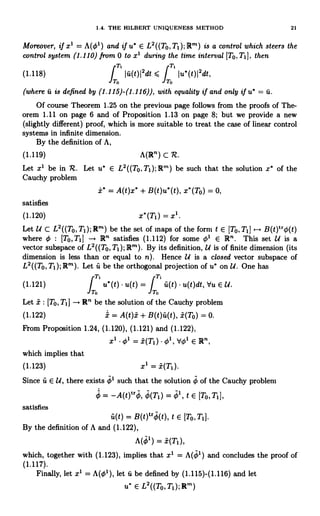
![2.1. TRANSPORT EQUATION 25
2.1.1. Well-posedness of the Cauchy problem. Let us first recall the
usual definition of solutions of the Cauchy problem
(2.4) yt + Y. = 0, t E (0,T), X E (0,L),
(2.5) y(t,0) = u(t), t E (0,T),
(2.6) y(0, x) = y°(x), x E (0, L).
where T > 0, y° E L2(0,L) and u E L'(0, T) are given. In order to motivate
this definition, let us first assume that there exists a function y of class C' on
[0,T] x [0,L] satisfying (2.4)-(2.5)-(2.6) in the usual sense. Let r E 10,T). Let
4) E C'([O,r] x [0,L1). We multiply (2.4) by ¢ and integrate the obtained identity
on 10, r] x [0, L]. Using (2.5), (2.6) and integrations by parts, one gets
- J J (¢, + 4=)ydxdt + J y(t, L)O(t, L)dt - I u(t)4(t,0)dt
0 0 0 0
+ f t y(r, x)4)(r, x)dx - f t y°(x)4)(0, x)dx = 0.
0 0
This equality leads to the following definition.
DEFINITION 2.1. Let T > 0, y° E L2(0, L) and u E L2(0,T) be given. A solu-
tion of the Cauchy problem (2.4)-(2.5)-(2.6) is a function y E C°([0,T];L2(0,L))
such that, for every r E [0, T] and for every 4) E C' ([0, r] x [0, L]) such that
(2.7) 4)(t, L) = 0, Vt E [0, r],
one has
r t
u(t)¢(t, 0)dt
(2.8) - f fo (41 + 4=)ydxdt - f0'r
0
f t y(r, x)4)(r, x)dx - f t y°(x)0(0, x)dx = 0.
+
0 0
This definition is also justified by the following proposition.
PROPOSITION 2.2. Let T > 0, y° E L2(0, L) and u E L2(0,T) be given. Let
us assume that y is a solution of the Cauchy problem (2.4)-(2.5)-(2.6) which is of
class C' in [0, T] x [0, L]. Then
(2.9) y° E C1([O, L]),
(2.10) u E C1([O,T]),
(2.11) y(0, x) = y°(x), Vx E [0, L],
(2.12) y(t,0) = u(t), Vt E (0, T],
(2.13) yl (t, x) + yx(t, x) = 0, V(t, X) E (0, TJ x [0, L].
Proof of Proposition 2.2. Let 0 E C' ([0, T] x [0, L]) vanish on ({0, T} x
[0, L]) fl ([0, T] x {0, L}). From Definition 2.1, we get, taking r := T,
fT
J'(0, + 4x)ydxdt = 0,
0](https://image.slidesharecdn.com/1270275-250526100502-0d891dfb/85/Control-And-Nonlinearity-Jeanmichel-Coron-44-320.jpg)
![26 2. LINEAR PARTIAL DIFFERENTIAL EQUATIONS
which, using integrations by parts, gives
(2.14)
1T1L
+ yl)4dxdt = 0.
Since the set 0 CI ([0,T] x [0, L]) vanishing on ({0, T} x [0, L]) fl ([0, T] x {0, L})
is dense in L'((O0IT .T)IL x (0, L)), (2.14) implies that
(2.15) (ye + y1)Ods:dt = 0, dO E Ll ((0, T) x (0, L)).
Taking 0 E L'((0, T) x (0, L)) defined by
(2.16) 0(t, x) := 1 if yt(t, x) + Y, (t, x) -> 0,
(2.17) 0(t. X) -1 if yt(t, x) + yx(t, x) < 0,
one gets
IT
(2.18) + y[dxdt 0,
which gives (2.13). Now let 0 E C' ([0,T] x [0, L]) be such that
(2.19) q(t. L) = 0, Vt E [0. T].
From (2.8) (with r = T), (2.13), (2.19) and integrations by parts, we get
T
(2.20)
I
(y(t, 0) - u(t))O(t, 0)dt + (y(0, x) - y(1(x))O(0, x)dx = 0.
0 0
Let 8 : C' ([0. T] x [0. L]) L'(0, T) x L' (0, L) be defined by
8(0) := (4(., 0), ¢(0, -))
One easily checks that
(2.21) 13({0 E C'([0, T] x [0,L]); (2.19) holds}) is dense in L'(0,T) x L'(0,L).
Proceeding as for the proof of (2.18), we deduce from (2.20) and (2.21)
f T Iy(t,0) - u(t)Idt
+ fT
Iy(0,x) - y°(x)Idx = 0.
o c0
This concludes the proof of Proposition 2.2.
EXERCISE 2.3. Let T > 0. y° E L2(0, L) and u E L2(0, T) be given. Let
y E C°([0.T]: L2(0, L)). Prove that y is a solution of the Cauchy problem (2.4)-
(2.5)-(2.6) if and only if. for every 0 E C' ([0, T] x [0, L]) such that
6(t, L) = 0, Vt E [0, T],
O(T, x) = 0, Vx E [0, L],
one has
T L
fT JL(0
fo 0
t + p,)ydxdt + u(t)O(t, 0)dt + y°(x)0(0, x)dx = 0.
W ith Definition 2.1, one has the following theorem.](https://image.slidesharecdn.com/1270275-250526100502-0d891dfb/85/Control-And-Nonlinearity-Jeanmichel-Coron-45-320.jpg)
![2.1. TRANSPORT EQUATION 27
THEOREM 2.4. Let T > 0. y° E L2(0, L) and u E L'(0, T) be given. Then the
Cauchy problem (2.4)-(2.5)-(2.6) has a unique solution. This solution satisfies
(2.22) IIy(r, )11L2(O.L) < IIy°IIL2(0,L) + II1UIIL2(°.T), Vr E [0,T].
Proof of Theorem 2.4. Let us first prove the uniqueness of the solution
to the Cauchy problem (2.4)-(2.5)-(2.6). Let us assume that yl and y2 are two
solutions of this problem. Let y := Y2 - yl. Then y E C°([0,T]; L2(0, L)) and, if
r E [0, T] and 0 E C' ([0, r] x [0, L]) satisfy (2.7), one has
rr
f' /1.
(2.23) - J f (¢t. + O=)ydxdt +
J
y(r, x)d(r, x)dx = 0.
0 0 0
Let r E [0, T]. Let (fn)nEN be a sequence of functions in C' (lib) such that
(2.24)
(2.25)
f = 0 on [L, +oc), Vn E N,
Jn1(0,L) -* y(r, ) in L2(0, L) as n -+ +oo.
For n E N, let ¢n E C' ([0, r] x [0, L]) be defined by
(2.26) 0,, (t, x) = fn (r + x - t), V(t, x) E [0, r] x [0, L].
By (2.24) and (2.26), (2.7) is satisfied for 0:= On. Moreover,
0nt + ¢nx = 0.
Hence, from (2.23) with O:= On and from (2.26), we get
L L
(2.27) f y(r,x)fn(x)dx = f y(r,x)On(r,x)dx = 0.
0 0
Letting n -. oc in (2.27), we get, using (2.25),
L
f I y(r, x)I2dx = 0.
Hence, for every r E [0,T]1 y(r, ) = 0.
Let us now give two proofs of the existence of a solution. The first one relies on
the fact that one is able to give an explicit solution! Let us define y : [0, T] x [0, L) -
R by
(2.28) y(t, x) := y°(x - t), V(t, x) E [0, T] x (0, L) such that t S x,
(2.29) y(t, x) := u(t - x), V(t, x) E [0, T] x (0, L) such that t > x.
Then one easily checks that this y is a solution of the Cauchy problem (2.4)-(2.5)-
(2.6). Moreover, this y satisfies (2.22).
Let us now give a second proof of the existence of a solution. This second proof
is longer than the first one, but can be used for much more general situations (see,
for example, Sections 2.2.1, 2.4.1, 2.5.1).
Let us first treat the case where
(2.30) u E C2([0,T]) and u(0) = 0,
(2.31) y° E H'(0, L) and y°(0) = 0.
Let A : D(A) C L2(0, L) -* L2(0, L) be the linear operator defined by
(2.32) D(A) :_ { f E H'(0, L); f (0) = 01,
(2.33) Af := -f_ Vf E D(A).](https://image.slidesharecdn.com/1270275-250526100502-0d891dfb/85/Control-And-Nonlinearity-Jeanmichel-Coron-46-320.jpg)
![28 2. LINEAR PARTIAL DIFFERENTIAL EQUATIONS
Note that
(2.34) D(A) is dense in L2(0, L),
(2.35) A is closed.
Let us recall that (2.35) means that ((f,Af); f E D(A)} is a closed subspace of
L2(0, L) x L2(0, L); see Definition A.1 on page 373. Moreover, A has the property
that, for every f E D(A),
(2.36) (Af, f)L2(o,L) = - f L f fxdx = -
f (L)2
< 0.
2
One easily checks that the adjoint A' of A is defined (see Definition A.3 on page 373)
by
D(A*) := If E H1(0, L); f (L) = 0},
A'f := fs, Vf E D(A*)
In particular, for every f E D(A'),
(2.37) (A*f,f)L2(O.L)= f Lffsdx=-f(0)2
<0.
Then, by a classical result on inhomogeneous initial value problems (Theo-
rem A.7 on page 375), (2.30), (2.31), (2.34), (2.35), (2.36) and (2.37), there exists
z E C' ([0, T]; L2(0, L)) n C°([0,T]; H1(0, L))
such that
(2.38) z(t,0) = 0, Vt E [0, T],
(2.39)
dt
= Az - u,
(2.40) y°.
Let y E C1([0, T]; L2(0, L)) n C°([0,T]; H1(0, L)) be defined by
(2.41) y(t,x) = z(t,x)+u(t), `d(t,x) E [0, T] x [0,L].
Let r E [0, T]. Let 0 E C1([0, T]; L2(0, L)) n C°([0, r]; H1(0, L)). Using (2.30),
(2.38), (2.39), (2.40) and (2.41), straightforward integrations by parts show that
(2.42) -
fr
f L(Ot + cx)ydxdt + y(t, L)q5(t, L)dt -
fr
u(t)O(t, 0)dt
0 0 0
L
+ f y(T, x)c(r, x)dx - fL
y°(x)0(0, x)dx = 0.
0 0
In particular, if we take 0:= YI[o,rjx[o,Lj, then
(2.43) fr
Iy(t, L)I2dt - fr
Iu(t)12dt + f L L
Iy(r,x)I2dx - f Iy°(x)I2dx = 0,
0 0 0 0
which implies that
(2.44) II y(r,')IIL2(o,L) < IIUIILa(o,T) + IIy°IIL2(O,L), YT E [0,T],
that is (2.22).](https://image.slidesharecdn.com/1270275-250526100502-0d891dfb/85/Control-And-Nonlinearity-Jeanmichel-Coron-47-320.jpg)
![2.1. TRANSPORT EQUATION 29
Now let y° E L2(0,L) and let u E L2(0,T). Let (yn)nEN be a sequence of
functions in D(A) such that
(2.45) yn -+ y° in L2(0, L) as n -* +oo.
Let (un)nEN be a sequence of functions in C2([0,T]) such that t (0) = 0 and
(2.46) un -p u in L2(0,T) as n +oo.
For n E N, let z,, E C1([0, T]; L2(0, L)) n C°([0, T]; H1(0, L)) be such that
(2.47) zn(t, 0) = 0, Vt E [0, T],
(2.48)
d = Azn - un,
(2.49) z-(0,') = Yon,
and let yn E C1([0,T];L2(0,L))nC°([0,TI;H1(0,L)) be defined by
(2.50) yn(t, x) = Z. (t, x) + un(t), `d(t, x) E [0, T] x [0, L].
Let r E [0, T]. Let 0 E C1([0, r] x [0, L]) be such that L) = 0. From (2.42)
(applied with y° yn, u u, and y := yn), one gets
r L t
(2.51) - J J (¢t + di=)yndxdt - J un(t)q (t, 0)dt
0 0 0
+ f yn(T, x)O(T, x)dx - f yo(x)0(0, x)dx = 0, do E N.
L L
0 0
From (2.44) (applied with y° := y°, u u,, and y := y,,),
(2.52) IIynIICa([0,T);L2(0,L)) 5 IIUnIIL2(o,T) + IIynIIL2(o,L).
Let (n, m) E N2. From (2.44) (applied with y° := y° - Y° , u := un - u,,, and
y:=yn-ym),
(2.53) llyn - yrIIC0([0,T];L2(o,L)) s Ilun - U. IIL2(0,T) + Ilyn - Y IIL2(0,L)
Rom (2.45), (2.46) and (2.53), (yn)nEN is a Cauchy sequence in C°([0, TI; L2(0, L)).
Hence there exists y E C°([0, T]; L2(0, L)) such that
(2.54) y,, - y in C°([0,T]; L2(0, L)) as n -, +oo.
From (2.51) and (2.54), one gets (2.8). From (2.52) and (2.54), one gets (2.22). This
concludes our second proof of the existence of a solution to the Cauchy problem
(2.4)-(2.5)-(2.6) satisfying (2.22).
2.1.2. Controllability. Let us now turn to the controllability of the control
system (2.2)-(2.3). We start with a natural definition of controllability.
DEFINITION 2.5. Let T > 0. The control system (2.2)-(2.3) is controllable in
time T if, for every y° E L2(0, L) and every y' E L2(0, L), there exists u E L2(0,T)
such that the solution y of the Cauchy problem (2.4)-(2.5)-(2.6) satisfies y(T, ) _
yl
With this definition we have the following theorem.
THEOREM 2.6. The control system (2.2)-(2.3) is controllable in time T if and
only if T > L.](https://image.slidesharecdn.com/1270275-250526100502-0d891dfb/85/Control-And-Nonlinearity-Jeanmichel-Coron-48-320.jpg)
![30 2. LINEAR PARTIAL DIFFERENTIAL EQUATIONS
REMARK 2.7. Let us point out that Theorem 2.6 on the previous page shows
that there is a condition on the time T in order to have controllability. Such
a phenomenon never appears for linear control systems in finite dimension. See
Theorem 1.16 on page 9. However, note that such a phenomenon can appear
for nonlinear control systems in finite dimension (see for instance Example 6.4 on
page 190).
We shall provide three different proofs of Theorem 2.6:
1. A proof based on the explicit solution y of the Cauchy problem (2.4)-(2.5)-
(2.6).
2. A proof based on the extension method.
3. A proof based on the duality between the controllability of a linear control
system and the observability of its adjoint.
2.1.2.1. Explicit solutions. Let us start the proof based on the explicit solution
of the Cauchy problem (2.4)-(2.5)-(2.6). We first take T E (0, L) and check that
the control system (2.2)-(2.3) is not controllable in time T. Let us define y° and y'
by
y°(x) = 1 and y' (x) = 0, Vx E [0, L].
Let u E L2(0, T). Then, by (2.28), the solution y of the Cauchy problem (2.4)-
(2.5)-(2.6) satisfies
y(T, x) = 1, x E (T, L).
In particular, y(T, ) 54 y'. This shows that the control system (2.2)-(2.3) is not
controllable in time T.
We now assume that T > L and show that the control system (2.2)-(2.3)
is controllable in time T. Let y° E L2(0, L) and y' E L2(0, L). Let us define
u E L2(0,T) by
u(t)=yl(T-t),tE(T-L,T),
u(t) = 0, t E (0, T - L).
Then, by (2.29), the solution y of the Cauchy problem (2.4)-(2.5)-(2.6) satisfies
y(T, x) = u(T - x) = y' (x), x E (0, L).
This shows that the control system (2.2)-(2.3) is controllable in time T.
2.1.2.2. Extension method. This method has been introduced in [425] by David
Russell. See also [426, Proof of Theorem 5.3, pages 688-690] by David Russell and
[332] by Walter Littman. We explain it on our control system (2.2)-(2.3) to prove
its controllability in time T if T > L. Let us first introduce a new definition.
DEFINITION 2.8. Let T > 0. The control system (2.2)-(2.3) is null controllable
in time T if, for every y° E L2(0, L), there exists u E L2(0, T) such that the solution
y of the Cauchy problem (2.4)-(2.5)-(2.6) satisfies y(T, ) = 0.
One has the following lemma.
LEMMA 2.9. The control system (2.2)-(2.3) is controllable in time T if and
only if it is null controllable in time T.](https://image.slidesharecdn.com/1270275-250526100502-0d891dfb/85/Control-And-Nonlinearity-Jeanmichel-Coron-49-320.jpg)
![2.1. TRANSPORT EQUATION 31
Proof of Lemma 2.9. The "only if" part is obvious. For the "if" part, let
us assume that the control system (2.2)-(2.3) is null controllable in time T. Let
y° E L2(0, L) and let yl E L2(0, L). Let us assume, for the moment, that there
exist 9° E L2(0, L) and u E L'(0, T) such that the solution y E C0([0, T]; L2(0, L))
of the Cauchy problem
(2.55) qt + 9, = 0, t E (0,T). x E (0, L),
(2.56) 9(t, 0) = u(t), t E (0,T),
(2.57) 9(0,x) _ 9°(x), x E (0, L),
satisfies
(2.58) y(T, x) := y' (x), x E (0, L).
Since the control system (2.2)-(2.3) is null controllable in time T, there exists
v. E L'(0, T) such that the solution y E C70 ([0,T]; L2(0, L)) of the Cauchy problem
(2.59) jt + yx = 0, t E (0, T), x E (0, L),
(2.60) y(t,0) = f, (t), t E (0,T),
(2.61) y(O,x) = y°(x) - 9°(x), x E (0,L),
satisfies
(2.62) (T, x) := 0, x E (0, L).
Let us define u E L2(0,T) by
(2.63) u it + ft.
From (2.55) to (2.57) and (2.59) to (2.61), the solution y E C°([0, T]; L2(0, L)) of
the Cauchy problem
yt + yr = 0, t E (0, T), x E (0, L),
y(t,0) = u(t), t E (0, T),
y(O, x) = y°(x), x E (0, L),
is y = + y. By (2.58) and by (2.62), y(T, ) = y'. Hence, as desired, the control u
steers the control system (2.2)-(2.3) from the state y° to the state y' during the time
interval [0, T]. It remains to prove the existence of 9° E L2(0, L) and v. E L2(0,T).
Let z E C°([0,T]; L2(0, L)) be the solution of the Cauchy problem
(2.64) zt + zx = 0, t E (0, T), x E (0, L),
(2.65) z(t, 0) = 0, t E (0, T),
(2.66) z(0, x) = y' (L - x), x E (0, L).
Note that from (2.64) we get z E H'((O,L);H-'(0,T)). In particular, is
well defined and
(2.67) L) E H-'(0,T).
In fact L) has more regularity than the one given by (2.67): one has
(2.68) L) E L2(0, T).
Property (2.68) can be seen by the two following methods.](https://image.slidesharecdn.com/1270275-250526100502-0d891dfb/85/Control-And-Nonlinearity-Jeanmichel-Coron-50-320.jpg)
![32 2. LINEAR PARTIAL DIFFERENTIAL EQUATIONS
- For the first one, one just uses the explicit expression of z; see (2.28) and
(2.29).
- For the second one, we start with the case where y' E H'(0, L) satisfies
y' (L) = 0. Then z E C'([0,T]; L2(0, L)) fl C°([0,T]; H'(0, L)). We multi-
ply (2.64) by z and integrate on [0, T] x [0, L]. Using (2.65) and (2.66), we
get
I
J
L z(T, x)2dx
-
f y' (x)2dx + z(t, L)2dt = 0.
I n particular,
(2.69) IIz(-,L)I(L2(0,T) <, IIY'IIV(0,L).
By density, (2.69) also holds if y' is only in L2(0, L), which completes the
second proof of (2.68).
We define y° E L2(0, L) and u E L2(0,T) by
9°(x) = z(T, L - x), x E (0, L),
u(t) = z(T - t, L), t E (0, T).
Then one easily checks that the solution y of the Cauchy problem (2.55)-(2.56)-
(2.57) is
(2.70) y(t, x) = z(T - t, L - x), t E (0, T), X E (0, L).
From (2.66) and (2.70), we get (2.58). This concludes the proof of Lemma 2.9.
REMARK 2.10. The fact that z(.,L) E L2(0,T) is sometimes called a hidden
regularity property; it does not follow directly from the regularity required on z,
i.e., z E C°([0,T]; L2(0, L)). Such a priori unexpected extra regularity properties
appear, as it is now well known, for hyperbolic equations (see in particular (2.307) on
page 68, [285] by Heinz-Otto Kreiss, [431, 432] by Reiko Sakamoto, [88, Theoreme
4.4, page 378] by Jacques Chazarain and Alain Piriou, [297, 298] by Irena Lasiecka
and Roberto Triggiani, [324, Theoreme 4.1, page 195] by Jacques-Louis Lions, [473]
by Daniel Tataru and [277, Chapter 2] by Vilmos Komornik. It also appears for our
Korteweg-de Vries control system studied below; see (2.140) due to Lionel Rosier
(407, Proposition 3.2, page 43].
Let us now introduce the definition of a solution to the Cauchy problem
(2.71) yc + yz = 0, (t, x) E (0, +oo) x R, y(0, x) = y°(x),
where y° is given in L2(R). With the same motivation as for Definition 2.1 on
page 25, one proposes the following definition.
DEFINITION 2.11. Let y° E L2(R). A solution of the Cauchy problem (2.71)
is a function y E C°([0,+oo);L2(R)) such that, for every T E [0, +oo), for every
R > 0 and for every ¢ E C' ([0, r] x R) such that
4(t, x) = 0, Vt E [0,r], dx E R such that IxI > R,
one has
/'r
fR
- l J (0c + gx)ydxdt + y(r,x)O(r,x)dx - J 0.
o R R](https://image.slidesharecdn.com/1270275-250526100502-0d891dfb/85/Control-And-Nonlinearity-Jeanmichel-Coron-51-320.jpg)
![2.1. TRANSPORT EQUATION 33
Then, adapting the proof of Theorem 2.4 on page 27, one has the following
proposition.
PROPOSITION 2.12. For every y° E L2(R), the Cauchy problem (2.71) has a
unique solution. This solution y satisfies
IIy(r,.)IIL2(R) = IIy°IIL2(R), `d-r E [0,+00).
In fact, as in the case of the Cauchy problem (2.4)-(2.5)-(2.6), one can give y
explicitly:
(2.72) y(t, x) = y°(x - t), t E (0, +oc), x E R.
Then the extension method goes as follows. Let y° E L2 (0, L). Let R > 0. Let
y° E L2(R) be such that
(2.73) 9°(x) = y°(x), x E (0, L),
(2.74) y-(x) = 0, x E (-oo, -R).
Let y E C°([0, +oo); L2(IR)) be the solution of the Cauchy problem
yt+y== 0,tE(0,+00),xER,
9(0, x) = y°(x), x E R.
Using (2.74) and the explicit expression (2.72) of the solution of the Cauchy problem
(2.71), one sees that
(2.75) 9(t,x)=0ifx<t-R.
Adapting the proofs of (2.68), one gets that
E L2(0,+00).
Let T >, L. Then one easily checks that the solution y E C°([0, T]; L2(0, L)) of the
Cauchy problem
yt + Y. = 0, t E (0, T), X E (0, L),
y(t,0) = 9(t, 0), t E (0,T),
y(0, x) = y°(x), x E (0, L),
is given by
(2.76) y(t, x) = y(t, x), t E (0, T), X E (0, L).
From (2.75), one gets y(T, ) = 0 if R < T- L. Hence the control t E (0, T) ,-+ y(t, 0)
steers the control system (2.2)-(2.3) from the state y° to 0 during the time interval
[0,T].
Of course, for our simple control system (2.2)-(2.3), the extension method seems
to be neither very interesting nor very different from the explicit method detailed
in Section 2.1.2.1 (taking R = 0 leads to the same control as in Section 2.1.2.1).
However, the extension method has some quite interesting advantages compared to
the explicit method for more complicated hyperbolic equations where the explicit
method cannot be easily applied; see, in particular, the paper [332] by Walter
Littman.
Let us also point out that the extension method is equally useful for our simple
control system (2.2)-(2.3) if one is interested in more regular solutions. Indeed, let
m E N, let us assume that y° E Hm(0, L) and that we want to steer the control](https://image.slidesharecdn.com/1270275-250526100502-0d891dfb/85/Control-And-Nonlinearity-Jeanmichel-Coron-52-320.jpg)
![34 2. LINEAR PARTIAL DIFFERENTIAL EQUATIONS
system (2.2)-(2.3) from y° to 0 in time T > L in such a way that the state always
remains in H' (0, L). Then it suffices to take R := T - L and to impose on y° to be
in Ht(iR). Note that if m > 1, one cannot take T = L, as shown in the following
exercise.
EXERCISE 2.13. Let m E N {0}. Let T = L. Let y° E Hm(O,L). Prove
that there exists u E L2(0,T) such that the solution y E Co Q0, T]; L'(0, L)) of the
Cauchy problem (2.4)-(2.5)-(2.6) satisfies
y(T, x) = 0, x E (0, L),
y(t, ) E H"'(0, L), Vt E [O,T],
if and only if
(y°)IWl(0) = 0, dj E {0, ... , m - 1}.
REMARK 2.14. Let us emphasize that there are strong links between the regu-
larity of the states and the regularity of the control: For r > 0, if the states are in
H''(0, L), one cannot have controllability with control u E H8(0, T) for
(2.77) s > r.
Moreover, (2.77) is optimal: For every T > L, for every y° E H'(0, L) and for
every yl E H''(0, L), there exists u E H''(O,T) such that the solution y of the
Cauchy problem (2.4)-(2.5)-(2.6) satisfies y(T, ) = yl and y E C°([0, T]; H''(0, L)).
Of course this problem of the links between the regularity of the states and the
regularity of the control often appears for partial differential equations; see, in par-
ticular, Theorem 9.4 on page 248. The optimal links often are still open problems;
see, for example, the Open Problem 9.6 on page 251.
2.1.2.3. Duality between controllability and observability. Let T > 0. Let us
define a linear map.FT : L2(0, T) L2(0, L) in the following way. Let u E L2(0, T).
Let y E C°([0, T]; L2(0, L)) be the solution of the Cauchy problem (2.4)-(2.5)-(2.6)
with y° := 0. Then
-17T(u) := y(T, )
One has the following lemma.
LEMMA 2.15. The control system (2.2)-(2.3) is controllable in time T if and
only if FT is onto.
Proof of Lemma 2.15. The "only if" part is obvious. Let us assume that
.PT is onto and prove that the control system (2.2)-(2.3) is controllable in time T.
Let y° E L2(0, L) and y' E L2(0, L). Let y be the solution of the Cauchy problem
(2.4)-(2.5)-(2.6) with u := 0. Since FT is onto, there exists u E L2(0,T) such that
.PT(u) = y' - y(T, ). Then the solution y of the Cauchy problem (2.4)-(2.5)-(2.6)
satisfies y(T, ) = y(T, ) + y' - y(T, ) = y', which concludes the proof of Lemma
2.15.
In order to decide whether FT is onto or not, we use the following classical result
of functional analysis (see e.g. [419, Theorem 4.15, page 97], or [71, Theoreme 11. 19,
pages 29-30] for the more general case of unbounded operators).](https://image.slidesharecdn.com/1270275-250526100502-0d891dfb/85/Control-And-Nonlinearity-Jeanmichel-Coron-53-320.jpg)
![2.1. TRANSPORT EQUATION 35
PROPOSITION 2.16. Let HI and H2 be two Hilbert spaces. Let F be a linear
continuous map from HI into H2. Then F is onto if and only if there exists c > 0
such that
(2.78) 11F*(x2)11H, > c11x211H2, dx2 E H2.
Moreover, if (2.78) holds for some c > 0, there exists a linear continuous map
from H2 into HI such that
F 0 9(x2) = x2, dx2 E H2,
IIQ(x2)IIH, s 1 IIx211H2, dx2 E H2.
C
In control theory, inequality (2.78) is called an "observability inequality". In
order to apply this proposition, we make explicit FT in the following lemma.
LEMMA 2.17. Let zT E H1(0, L) be such that
(2.79) zT(L) = 0.
Let z E CI ([0, T]; L2(0, L)) n C°([0, T]; H1(0, L)) be the (unique) solution of
(2.80) z, + zx = 0,
(2.81) z(t, L) = 0, Vt E [0, T],
(2.82) z(T. ) = zT
Then
(2.83) FT(zT) = 0).
Proof of Lemma 2.17. Let us first point out that the proof of the existence
and uniqueness of z E C'([0,T];L2(0,L)) nC°([0,T];H'(0,L)) satisfying (2.80)
to (2.82) is the same as the proof of the existence and uniqueness of the solution
of (2.38) to (2.40). In fact, if z E C' ([0, T]; L2(0, L)) n Co([O, TI; H'(0, L)) is the
solution of
z(t, 0) = 0, Vt E [0, T[,
dt = Az,
dt
z(0, x) = zT (L - x), tlx E [0, L],
then
z(t, x) = z(T - t, L - x), V(t, X) E [0, T] x [0, L].
Let u E C2([0,T]) be such that u(0) = 0. Let
y E CI([O,T];L2(0,L))nC°([0,T];H1(0,L))
be such that
(2.84) yt + y= = 0,
(2.85) y(t,0) = u(t), Vt E [0, T],
(2.86) 0.](https://image.slidesharecdn.com/1270275-250526100502-0d891dfb/85/Control-And-Nonlinearity-Jeanmichel-Coron-54-320.jpg)

![NO. XXXVII.—GRANADA.
The city of Granada[252] has twelve gates; and is about eight
miles round, defended by high walls, flanked with a multitude of
towers. Its situation is of a mixed kind; some parts of it being upon
the mountain, and other parts in the plain. The mountainous part
stands upon three small eminences; the one is called Albrezzin;
which was inhabited by the Moors that were driven out of Baezza by
the Christians. The second is called Alcazebe; and the third
Alhambra. This last is separated from the other parts by a valley,
through which the river Darro runs; and it is also fortified with
strong walls, in such a manner as to command all the rest of the
city. The greatest part of this fortified spot of ground is taken up
with a most sumptuous palace of the Moorish kings. This palace is
built with square stones of great dimensions; and is fortified with
strong walls and prodigious large towers; and the whole is of such
an extent as to be capable of holding a very numerous garrison. The
outside has exactly the appearance of an immense romantic old
castle; but it is exceedingly magnificent within.
But before we enter, we must take notice of a remarkable piece of
sculpture over the great gate; there is the figure of a large key of a
castle-gate, and at some distance above it, there is an arm reaching
towards it; and the signification of this emblematical marble basso-
relief is this:—that the castles will never be taken till the arm can
reach the key.
Upon entering, not only the portico is of marble, but the
apartments also are incrusted with marble, jasper, and porphyry, and
the beams curiously carved, painted, and gilt; and the ceilings
ornamented with pieces of foliage in stucco. The next place you
come to is an oblong-square court, paved with marble, at each angle
of which there is a fountain, and in the middle there is a very fine](https://image.slidesharecdn.com/1270275-250526100502-0d891dfb/85/Control-And-Nonlinearity-Jeanmichel-Coron-56-320.jpg)
![wear and tear of centuries, the shock of earthquakes, the violence of
war, and the quiet and no less baneful pilfering of the tasteful
traveller.
There is a Moorish tradition, that a king who built this mighty pile
was skilled in the occult sciences, and furnished himself with gold
and silver for the purpose by means of alchymy; certainly never was
there an edifice accomplished in a superior style of barbaric
magnificence; and the stranger who, even at the present day,
wanders among its silent and deserted courts and ruined halls,
gazes with astonishment at its gilded and fretted domes and
luxurious decorations, still retaining their brilliancy and beauty in
spite of the ravages of time.
The Alhamrā, usually, but erroneously, denominated the Alhambra,
is a vast pile of building about two thousand three hundred English
feet in length; and its breadth, which is the same throughout, is
about six hundred feet. It was erected by Mūhammed Abū Abdillāh,
surnamed Alghālib Billāh, who superintended the edifice himself,
and, when it was completed, made it the royal residence.
Although the glory and prosperity of Granada may be said to have
departed with its old inhabitants, yet, happily, it still retains, in pretty
good preservation, what formed its chief ornament in the time of the
Moors. This is the Alhambra, the royal alcazar, or fortress and
palace, which was founded by Mūhammed Abū. Abdillāh Ben Nasz,
the second sovereign of Granada, defrayed the expense of the works
by a tribute imposed upon his conquered subjects. He superintended
the building in person, and when it was completed, he made it a
royal residence[253]. The immediate successors of this prince also
took delight in embellishing and making additions to the fabric. Since
the conquest of Granada by the Christians, the Alhambra has
undergone some alterations. It was for a time occasionally inhabited
by the kings of Spain. Charles the Fifth caused a magnificent palace
to be commenced within the walls; but owing to his wars and
frequent absences from Spain, or, as some accounts say, to repeated](https://image.slidesharecdn.com/1270275-250526100502-0d891dfb/85/Control-And-Nonlinearity-Jeanmichel-Coron-58-320.jpg)

![itself, which is covered with an immense number of trees laden with
fruit and blossoms; while, on the south, it is bounded by mountains,
whose lofty summits are crowned with perpetual snows, whence
issue the springs and streams that diffuse both health and coolness
through the city of Granada."
"But," in the language of Mr. Swinburne, "the glories of Granada
have passed away; its streets are choked with filth; its woods
destroyed; its territory depopulated; its trade lost. In a word,
everything, except the church and the law, is in the most deplorable
condition[254]."](https://image.slidesharecdn.com/1270275-250526100502-0d891dfb/85/Control-And-Nonlinearity-Jeanmichel-Coron-63-320.jpg)
![NO. XXXVIII.—GNIDOS.
This was a maritime city of Asia Minor, founded by the Dorians,
and much known on account of a victory, which Conon gained over
the Lacedemonians. Conon was an Athenian, having the command
of the Persian fleet; Pisander, brother-in-law of Agesilaus, of the
Lacedemonian. Conon's fleet consisted of ninety galleys; that of
Pisander something less. They came in view of each other near
Gnidos. Conon took fifty of the enemy's ships. The allies of the
Spartans fled, and their chief admiral died fighting to the last, sword
in hand.
Gnidos was famed for having produced the most renowned
sculptors and architects of Greece; amongst whom were Sostratus
and Sesostris, who built the celebrated light-tower on the isle of
Pharos, considered one of the seven wonders of the world, and
whence all similar edifices were afterwards denominated.
Venus, surnamed the Gnidian, was the chief deity of this place,
where she had a temple, greatly celebrated for a marble statue of
the goddess. This beautiful image was the masterpiece of Praxiteles,
who had infused into it all the soft graces and attractions of his
favourite Phryne; and it became so celebrated, that travellers visited
the spot with great eagerness. It represented the goddess in her
naked graces, erect in posture, and with her right hand covering her
waist; but every feature and every part was so naturally expressed,
that the whole seemed to be animated[255].
"We were shown, as we passed by," says Anacharsis, "the house
in which Eudoxus, the astronomer, made his observations; and soon
after found ourselves in the presence of the celebrated Venus of
Praxiteles. This statue had just been placed in the middle of a small
temple, which received light by two opposite doors, in order that a](https://image.slidesharecdn.com/1270275-250526100502-0d891dfb/85/Control-And-Nonlinearity-Jeanmichel-Coron-64-320.jpg)
![a large temple, also in ruins, and still more overgrown with bushes.
The frieze and cornice of this temple, which lie amongst the rubbish,
are of the highest and most beautiful workmanship. A little to the
north of this stood a smaller temple, of grey veined marble, whereof
almost every vestige is obliterated.
Several arches of rough masonry, and a breast-work, support a
large square area, in which are the remains of a long colonnade, of
white marble, and of the Doric order, the ruins of an ancient stoa. Of
the Acropolis nothing is left but a few walls of strong brown
stone[256].
Besides these there are the remains of two aqueducts;
undistinguishable pieces of wall, some three, some five, eight, ten
feet from the ground; columns plain, and fluted; a few small octagon
altars, and heaps of stones. Along the sea-shore lie pieces of black
marble[257].
Whenever the ground is clear[258], it is ploughed by the peasantry
around, who frequently stop here for days together, in chambers of
the ruins and caves of the rocks. The Turks and Greeks have long
resorted thither, as to a quarry, for the building materials afforded by
the remains.
The British consul at Rhodes states, that a fine colossal statue of
marble is still standing in the centre of the orchestra belonging to
the theatre, the head of which the Turks have broken off; but he
remembers it when in a perfect state. Mr. Walpole brought away the
torso of a male statue, and which has since been added to the
collection of Greek marbles at Cambridge[259].](https://image.slidesharecdn.com/1270275-250526100502-0d891dfb/85/Control-And-Nonlinearity-Jeanmichel-Coron-66-320.jpg)
![NO. XXXIX.—HELIOPOLIS.
This city was situated in that part of Egypt which is called the
Delta. It was named Heliopolis, city of the sun, from the
circumstance of there being a temple dedicated to the sun there;
and here, according to historians, originated the tale in respect to
the phœnix.
At this place, Cambyses, king of Persia, committed a very great
extravagance; for he burned its temple, demolished all the palaces,
and destroyed most of the monuments of antiquity that were then in
it. Some obelisks, however, escaped his fury, which are still to be
seen; others were transported to Rome.
In this city[260] Sesostris built two obelisks of extreme hard stone,
brought from the quarries of Syene, at the extremity of Egypt. They
were each 120 cubits high; that is, 30 fathoms, or 180 feet. The
emperor Augustus, having made Egypt a province of the Roman
empire, caused these two obelisks to be transplanted to Rome, one
of which was afterwards broken to pieces. He durst not venture
upon a third, which was of monstrous size. It was made in the reign
of Rameses; and it is said that 20,000 men were employed in the
cutting of it. Constantius, more daring than Augustus, ordered it to
be removed to Rome. Two of these obelisks are still to be seen; as
well as another of 100 cubits, or 25 fathoms high, and 8 cubits, or 2
fathoms in diameter. Caius Cæsar had it taken from Egypt in a ship
of so odd a form, that, according to Pliny, the like had never been
seen.
At Heliopolis, there remains only a solitary sphinx and an obelisk,
to mark the site of the city of the sun, where Moses, Herodotus, and
Plato, are said to have been instructed in the learning of the
Egyptians; whose learning and arts brought even Greece for a pupil,](https://image.slidesharecdn.com/1270275-250526100502-0d891dfb/85/Control-And-Nonlinearity-Jeanmichel-Coron-67-320.jpg)
![and whose empire, says Bossuet, in regard to Egypt in general, had
a character distinct from any other.
"This kingdom (says Rollin) bestowed its noblest labours and
finest arts on the improving of mankind; and Greece was so sensible
of this, that its most illustrious men,—as Homer, Pythagoras, Plato,
even its great legislators, Lycurgus and Solon, with many more,—
travelled into Egypt to complete their studies, and draw from that
fountain whatever was most rare and valuable in every kind of
learning. God himself has given this kingdom a glorious testimony,
when, praising Moses, he says of him, that 'he was learned in all the
wisdom of the Egyptians.' Such was the desire for encouraging the
growth of scientific pursuits, that the discoverers of any useful
invention received rewards suitable to their skill and labour. They
studied natural history, geometry, and astronomy, and what is
worthy of remark, they were so far masters of the latter science, as
to be aware of the period required for the earth's annual revolutions,
and fixed the year at 365 days 6 hours—a period which remained
unaltered till the very recent change of the style. They likewise
studied and improved the science of physic, in which they attained a
certain proficiency. The persevering ingenuity and industry of the
Egyptians are attested by the remains of their great works of art,
which could not well be surpassed in modern times; and although
their working classes were doomed to engage in the occupations of
their fathers, and no others, as is still the custom in India, society
might thereby be hampered, but the practice of handicrafts would be
certainly improved. The Egyptians were also the first people who
were acquainted with the process of communicating information by
means of writing, or engraving on stone and metal; and were,
consequently, the first who formed books and collected libraries.
These repositories of learning they guarded with scrupulous care,
and the titles they bore, naturally inspired a desire to enter them.
They were called the "Office for the Diseases of the Soul," and that
very justly; because the soul was there cured of ignorance, which, it
will be allowed, is the source of many of the maladies of our mental
faculties[261]."](https://image.slidesharecdn.com/1270275-250526100502-0d891dfb/85/Control-And-Nonlinearity-Jeanmichel-Coron-68-320.jpg)

![NO. XL.—HERCULANEUM.
"It is characteristic of the noblest natures and the finest
imaginations," says an elegant writer[262], "to love to explore the
vestiges of antiquity, and to dwell in times that are no more. The
first is the domain of the imaginative affections alone; we can carry
none of our baser passions with us thither. The antiquary is often
spoken of as being of a peculiar construction of intellect, which
makes him think and feel differently from other people. But, in truth,
the spirit of antiquarianism is one of the most universal of human
tendencies. There is, perhaps, scarcely any person, for example, not
utterly stupid or sophisticated, who would not feel a strange thrill
come over him in the wonderful scenes these volumes describe.
Looking round upon the long ruined city, who would not, for the
moment, utterly forget the seventeen centuries that had revolved
since Herculaneum and Pompeii were part and parcel of the world,
moving to and fro along its streets! It would not be deemed a mere
fever of curiosity that would occupy the mind,—an impatience to pry
into every hole and corner of a scene at once so old and so new.
Besides all that, there would be a sense of the actual presence of
those past times, almost like the illusion of a dream. There is, in
fact, perhaps no spot of interest on the globe, which would be found
to strike so deep an impression into so many minds."
Herculaneum is an ancient city of Italy, situated in the Bay of
Naples, and supposed to have been founded by Hercules, or in
honour of him, 1250 years before the Christian era.[263] "This city,"
says Strabo, "and its next neighbour, Pompeii, on the river Sarnus,
were originally held by the Osci, then by the Tyrrhenians and
Pelasgians, then by the Samnites, who, in their turn, took possession
of it, and retained it ever after."](https://image.slidesharecdn.com/1270275-250526100502-0d891dfb/85/Control-And-Nonlinearity-Jeanmichel-Coron-70-320.jpg)
![The adjacent country[264] was distinguished in all ages for its
romantic loveliness and beauty. The whole coast, as far as Naples,
was studded with villas, and Vesuvius, whose fires had been long
quiescent, was itself covered with them. Villages were also scattered
along the shores, and the scene presented the appearance of one
vast city, cut into a number of sections by the luxuriant vegetation of
the paradise in which it was embosomed.
The following epigram of Martial gives an animated view of the
scene, previous to the dreadful catastrophe, which so blasted this
fair page of Nature's book:—
Here verdant vines o'erspread Vesuvius' sides;
The generous grape here pour'd her purple tides.
This Bacchus loved beyond his native scene;
Here dancing satyrs joy'd to trip the green.
Far more than Sparta this in Venus' grace;
And great Alcides once renown'd the place;
Now flaming embers spread dire waste around,
And gods regret that gods can so confound.
The scene of luxurious beauty[265] and tranquillity above
described was doomed to cease, and the subterranean fire which
had been from time immemorial extinct in this quarter, again
resumed its former channel of escape. The long period of rest, which
had preceded this event, seems to have augmented the energies of
the volcano, and prepared it for the terrible explosion. The first
intimation of this was the occurrence of an earthquake, in the year
63 after Christ, which threw down a considerable portion of Pompeii,
and also did great damage to Herculaneum. In the year following,
another severe shock was felt, which extended to Naples, where the
Roman emperor Nero was at the time exhibiting as a vocalist. The
building in which he performed was destroyed, but unfortunately the
musician had left it. These presages of the approaching catastrophe
were frequently repeated, until, in A. D. 79 (Aug. 24), they ended in
the great eruption. Fortunately we are in possession of a narrative of
the awful scene, by an eye-witness;—Pliny the younger, who was at
the time at Misenum, with the Roman fleet, commanded by his](https://image.slidesharecdn.com/1270275-250526100502-0d891dfb/85/Control-And-Nonlinearity-Jeanmichel-Coron-71-320.jpg)
![had repeatedly shaken all the small towns, and even cities in the
neighbourhood, was increasing every moment. I rose to go and
awake my mother, and met her hastily entering my apartment to
awaken me.
"We descended into the court, and sat down there. Not to lose
time, I sent for my Livy. I read, meditated, and made extracts, as I
would have done in my chamber. Was this firmness, or was it
imprudence? I know not now; but I was then very young![266] At the
same instant one of my uncle's friends, just arrived from Spain,
came to visit him. He reproached my mother with her security, and
me with my audacity. The houses, however, were shaking in so
violent a manner, that we resolved to quit Misenum. The people
followed us in consternation.
"As soon as we had got out of the town we stopped. Here we
found new prodigies and new terrors. The shore, which was
continually extending itself, and covered with fishes left dry on it,
was heaving every moment, and repelling to a great distance the
enraged sea which fell back upon itself; whilst before us, from the
limits of the horizon, advanced a black cloud, loaded with dull fires,
which were incessantly rending it, and darting forth large flashes of
lightning. The cloud descended and enveloped all the sea, it was
impossible any longer to discern either the isle of Caprea, or the
promontory of Misenum. 'Save yourself, my dear son,' cried my
mother; 'save yourself; it is your duty; for you can, and you are
young: but as for me, bulky as I am, and enfeebled with years,
provided I am not the cause of thy death, I die contented.'—'Mother,
there is no safety for me but with you.'—I took my mother by the
hand, and drew her along.—'O my son,' said she in tears, 'I delay
thy flight.'
"Already the ashes began to fall; I turned my head; a thick cloud
was rushing precipitately towards us.—'Mother,' said I, 'let us quit
the high road; the crowd will stifle us in that darkness which is
pursuing us.' Scarcely had we left the high road before it was night,](https://image.slidesharecdn.com/1270275-250526100502-0d891dfb/85/Control-And-Nonlinearity-Jeanmichel-Coron-73-320.jpg)
![My uncle hesitated whether he should return from whence he came,
or put out to sea. Fortune favours courage (exclaimed he), let us
turn towards Pomponianus. Pomponianus was at Stabiæ. My uncle
found him all trembling: embraced and encouraged him, and to
comfort him by his security, asked for a bath, then sat down to table
and supped cheerfully; or, at least, which does not show less
fortitude, with all the appearance of cheerfulness.
"In the mean time Vesuvius was taking fire on every side, amid
the thick darkness. 'It is the villages which have been abandoned
that are burning,' said my uncle to the crowd about him, to
endeavour to quiet them. He then went to bed, and fell asleep. He
was in the profoundest sleep, when the court of the house began to
fill with cinders; and all the passages were nearly closed up. They
run to him; and were obliged to awaken him. He rises, joins
Pomponianus, and deliberates with him and his attendants what is
best to be done, whether it would be safest to remain in the house
or fly into the country. They chose the latter measure.
"They departed instantly therefore from the town, and the only
precaution they could take was to cover their heads with pillows.
The day was reviving everywhere else; but there it continued night;
horrible night! the fire from the cloud alone enlightened it. My uncle
wished to gain the shore, notwithstanding the sea was still
tremendous. He descended, drank some water, had a sheet spread,
and lay down on it. On a sudden, violent flames, preceded by a
sulphureous odour, shot forth with a prodigious brightness, and
made every one take to flight. My uncle, supported by two slaves,
arose; but suddenly, suffocated by the vapour, he fell[267],—and
Pliny was no more[268]."
If this visitation affected Misenum in so terrible a manner, what
must have been the situation of the unfortunate inhabitants of
Pompeii and Herculaneum, so near its focus? The emperor Titus
here found an opportunity for the exercise of his humanity. He
hastened to the scene of affliction, appointed curatores[269], persons](https://image.slidesharecdn.com/1270275-250526100502-0d891dfb/85/Control-And-Nonlinearity-Jeanmichel-Coron-75-320.jpg)
![of consular dignity, to set up the ruined buildings, and take charge of
the effects. He personally encouraged the desponding, and
alleviated the misery of the sufferers; whilst a calamity of an equally
melancholy description recalled him to Rome; where a most
destructive fire, laying waste nearly half the city, and raging three
days without interruption, was succeeded by a pestilence, which for
some time carried off ten thousand persons every day!
Herculaneum and Pompeii rose again from their ruins in the reign
of Titus; and they still existed with some remains of splendour under
Hadrian[270]. The beautiful characters of the inscription, traced out
on the base of the equestrian statue of Marcus Nonius Balbus, son of
Marcus, are an evident proof of its existence at that period. They
were found under the reign of the Antonines. In the geographical
monument, known under the name of Peutinger's chart, which is of
a date posterior to the reign of Constantine, that is to say in the
commencement of the 4th century, Herculaneum and Pompeii were
still standing, and then inhabited; but in the Itinerary, improperly
ascribed to Antoninus, neither of these two cities is noticed; from
which it may be conjectured, that their entire ruin must have taken
place in the interval between the time when Peutinger's chart was
constructed, and that when the above Itinerary was composed.
The eruption, which took place in 471, occasioned the most
dreadful ravages. It is very probable that the cities of Herculaneum
and Pompeii disappeared at that period, and that no more traces of
them were left.
It appears, by the observation of Sir W. Hamilton[271], that the
matter, which covers the ancient town of Herculaneum, is not the
produce of one eruption only; but there are evident marks that the
matter of six eruptions has taken its course over that which lie
immediately above the town; and which was the cause of its
destruction. These strata are either of lava or burnt matter, with
veins of good soil between them. The stratum of erupted matter that
immediately covers the town, and with which the theatre and most](https://image.slidesharecdn.com/1270275-250526100502-0d891dfb/85/Control-And-Nonlinearity-Jeanmichel-Coron-76-320.jpg)
![of the houses were filled, is not of that sort of vitrified matter, called
lava, but of a sort of soft stone composed of pumice, ashes, and
burnt matter. It is exactly of the same nature with what is called the
Naples stone. The Italians call it tufa; and it is in general use for
building.
Herculaneum was covered with lava; Pompeii with pumice stone; yet
the houses of the latter were built of lava; the product of former
eruptions.
All memorials of the devoted cities were lost[272]; and discussions,
over the places they had once occupied, were excited only by some
obscure passages in the classical authors. Six successive eruptions
contributed to lay them still deeper under the surface. But after that
period had elapsed, a peasant digging a well beside his cottage in
1711, obtained some fragments of coloured marble, which attracted
attention. Regular excavations were made, under the
superintendence of Stendardo, an architect of Naples; and a statue
of Hercules, of Greek workmanship, and also a mutilated one of
Cleopatra, were drawn from what proved to be a temple in the
centre of the ancient Herculaneum.
It may be well conceived with what interest the intelligence was
received, that a Roman city had been discovered, which, safely
entombed under-ground, had thus escaped the barbarian Goths and
Vandals, who ravaged Italy, or the sacrilegious hands of modern
pillagers.
The remains of several public buildings have been discovered[273],
which have possibly suffered from subsequent convulsions. Among
these are two temples; one of them one hundred and fifty feet by
sixty, in which was found a statue of Jupiter. A more extensive
edifice stood opposite to them; forming a rectangle of two hundred
and twenty-eight feet by one hundred and thirty-two, supposed to
have been appropriated for the courts of justice. The arches of a
portico surrounding it were supported by columns; within, it was
paved with marble; the walls were painted in fresco; and bronze](https://image.slidesharecdn.com/1270275-250526100502-0d891dfb/85/Control-And-Nonlinearity-Jeanmichel-Coron-77-320.jpg)
![statues stood between forty columns under the roof. A theatre was
found nearly entire; very little had been displaced; and we see in it
one of the best specimens extant of the architecture of the ancients.
The greatest diameter of the theatre is two hundred and thirty-four
feet, whence it is computed, that it could contain ten thousand
persons, which proves the great population of the city.
This theatre was rich in antiquities[274], independent of the
ornamental part. Statues, occupying niches, represented the Muses;
scenic masks were imitated on the entablatures; and inscriptions
were engraven on different places. Analogous to the last were
several large alphabetical Roman characters in bronze; and a
number of smaller size, which had probably been connected in some
conspicuous situation. A metallic car was found, with four bronze
horses attached to it, nearly of the natural size; but all in such a
state of decay, that only one, and the spokes of the wheels, also in
metal, could be preserved. A beautiful white marble statue of Venus,
only eighteen inches high, in the same attitude as the famous Venus
de Medicis, was recovered; and either here, or in the immediate
vicinity, was found a colossal bronze statue of Vespasian, filled with
lead, which twelve men were unable to move.
Besides many objects entire, there were numerous fragments of
others, extremely interesting; which had been originally impaired, or
were injured by attempts to remove them.
When we reflect, that sixteen hundred years have elapsed since
the destruction of this city[275], an interval which has been marked
by numerous revolutions, both in the political and mental state of
Europe, a high degree of interest must be experienced in
contemplating the venerable remains, recovered from the
subterraneous city of Herculaneum. Pliny, the younger, in his letters,
brings the Romans, their occupations, manners, and customs, before
us. He pictures in feeling terms the death of his uncle, who perished
in the same eruption as the city we now describe; and that event is
brought to our immediate notice by those very things which it was](https://image.slidesharecdn.com/1270275-250526100502-0d891dfb/85/Control-And-Nonlinearity-Jeanmichel-Coron-78-320.jpg)
![the means of preserving. Among these we see the various articles
which administered to the necessities and the pleasures of the
inhabitants, the emblems of their religious sentiments, and the very
manners and customs of domestic life.
These curiosities consist not only of statues, busts, altars,
inscriptions, and other ornamental appendages of Grecian opulence
and luxury; but also comprehend an entire assortment of the
domestic, musical, and surgical instruments; tripods of elegant form
and exquisite execution; lamps in endless variety; vases and basins
of noble dimensions; chandeliers of the most beautiful shapes,
looking-glasses of polished metal; coloured glass, so hard, clear, and
well stained, as to appear like emeralds, sapphires, and other
precious stones; a kitchen completely fitted up with copper pans
lined with silver, kettles, cisterns for heating water, and every utensil
necessary for culinary purposes; also specimens of various sorts of
combustibles, retaining their form though burnt to a cinder. By an
inscription, too, we learn that Herculaneum contained no less than
nine hundred houses of entertainment, such as we call taverns.
Articles of glass, artificial gems, vases, tripods, candelabra, lamps,
urns, dice, and dice-boxes; various articles of dress and ornaments;
surgical instruments, weights and measures, carpenters' and
masons' tools; but no musical instruments except the sistrum,
cymbals, and flutes of bone and ivory.
Fragments of columns of various coloured marble and beautiful
mosaic pavements were also found disseminated among the ruins;
and numerous sacrificial implements, such as pateræ, tripods, cups,
and vases, were recovered in excellent preservation, and even some
of the knives with which the victims are conjectured to have been
slaughtered.
The ancient pictures of Herculaneum[276] are of the utmost
interest; not only from the freshness and colour, but from the nature
of the subjects they represent. All are executed in fresco; they are
exclusively on the walls, and generally on a black or red ground.](https://image.slidesharecdn.com/1270275-250526100502-0d891dfb/85/Control-And-Nonlinearity-Jeanmichel-Coron-79-320.jpg)
![Some are of animated beings large as life; but the majority are in
miniature. Every different subject of antiquity is depicted here;
deities, human figures, animals, landscapes, foreign and domestic,
and a variety of grotesque beings; sports and pastimes, theatrical
performances, sacrifices, all enter the catalogue.
In regard to the statues found[277], some are colossal, some of
the natural size, and some in miniature; and the materials of their
formation are either clay, marble, or bronze. They represent all
different objects, divinities, heroes, or distinguished persons; and in
the same substances, especially bronze, there are the figures of
many animals.
It is not probable that the best paintings of ancient Greece and
Italy[278] were deposited in Herculaneum or Pompeii, which were
towns of the second order, and unlikely to possess the master-pieces
of the chief artists, which were usually destined to adorn the more
celebrated temples or the palaces of kings and emperors. Their best
statues are correct in their proportions, and elegant in their forms;
but their paintings are not correct in their proportions, and are,
comparatively, inelegant in their forms.
A few rare medals also have been found among these ruins, the
most curious of which is a gold medallion of Augustus, struck in
Sicily in the fifteenth year of his reign.
Nor must we omit one of the greatest curiosities, preserved at
Portici[279]. This consists of a cement of cinders, which in one of the
eruptions of Vesuvius surprised a woman, and totally enveloped her.
This cement, compressed and hardened by time around her body,
has become a complete mould of it, and in the pieces here
preserved, we see a perfect impression of the different parts to
which it adhered. One represents half a bosom, which is of exquisite
beauty; another a shoulder, a third a portion of her shape, and all
concur in revealing to us that this woman was young; that she was](https://image.slidesharecdn.com/1270275-250526100502-0d891dfb/85/Control-And-Nonlinearity-Jeanmichel-Coron-80-320.jpg)
![tall and well made, and even that she had escaped in her chemise,
for some of the linen was still adhering to the ashes.
Though the city was destroyed[280] in the manner we have
related, remarkably few skeletons have been found, though many
were discovered in the streets of Pompeii; but one appears under
the threshold of a door with a bag of money in his hand, as if in the
attitude of escaping, leaving its impression in the surrounding
volcanic matter.
These and other valuable antiquities are preserved in the museum
at Portici, which occupies the site of ancient Herculaneum, and in
the Museo Borbonico at Naples. For details in respect to which, we
must refer to the numerous books that have described them.
One of the most interesting departments of this unique collection
is that of the Papyri, or MSS., discovered in the excavation of
Herculaneum. The ancients did not bind their books (which, of
course, were all MSS.) like us, but rolled them up in scrolls. When
those of Herculaneum were discovered, they presented, as they still
do, the appearance of burnt bricks, or cylindrical pieces of charcoal,
which they had acquired from the action of the heat contained in the
lava, that buried the whole city. They seemed quite solid to the eye
and touch; yet an ingenious monk discovered a process of detaching
leaf from leaf, and unrolling them, by which they could be read
without much difficulty. It is, nevertheless, to be regretted, that so
little success has followed the labours of those who have attempted
to unrol them. Some portions, however, have been unrolled, and the
titles of about 400 of the least injured have been read. They are, for
the most part, of little importance; but all entirely new, and chiefly
relating to music, rhetoric, and cookery. The obliterations and
corrections are numerous, so that there is a probability of their being
original manuscripts. There are two volumes of Epicurus "on Virtue,"
and the rest are, for the most part, productions of the same school
of writers. Only a very few are written in Latin, almost all being in
Greek. All were found in the library of one individual, and in a](https://image.slidesharecdn.com/1270275-250526100502-0d891dfb/85/Control-And-Nonlinearity-Jeanmichel-Coron-81-320.jpg)