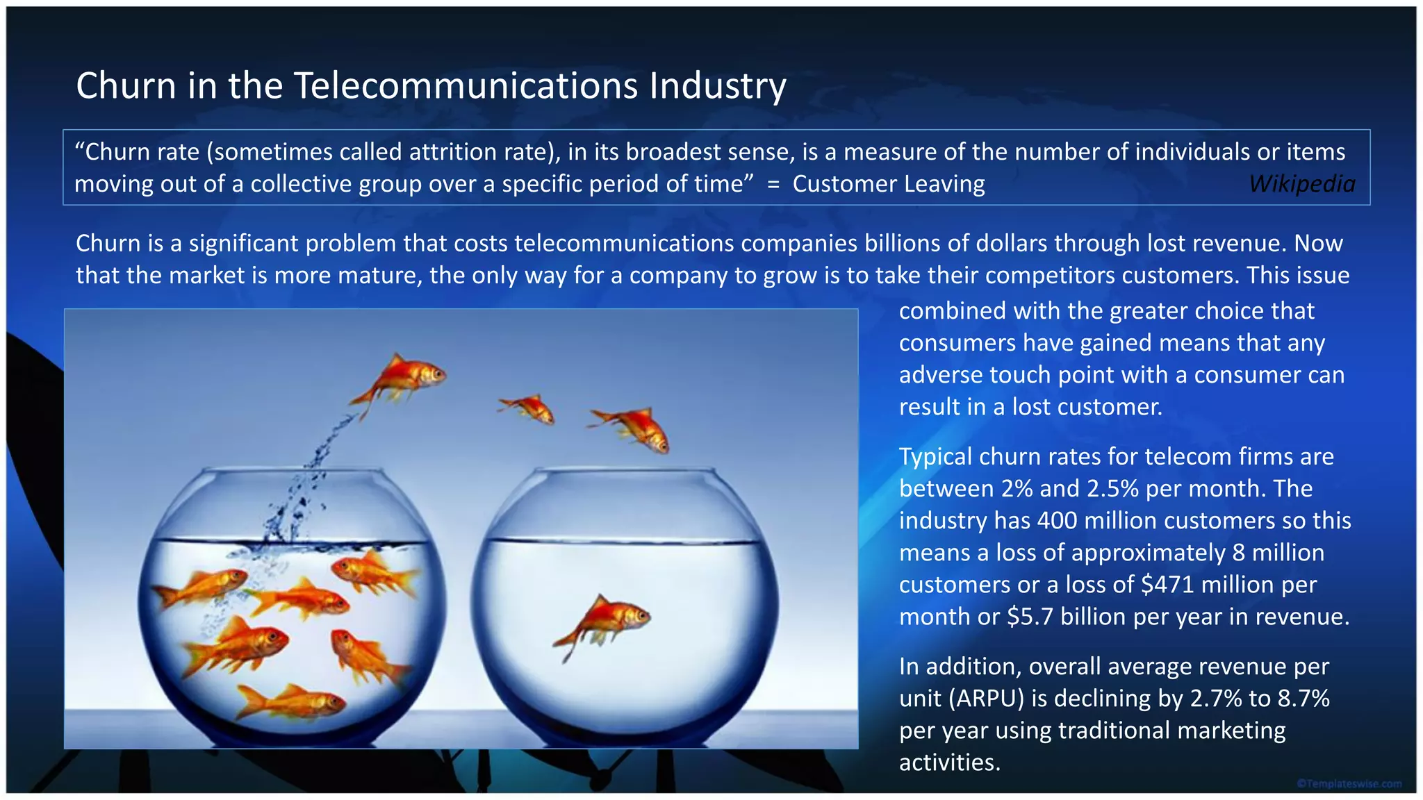
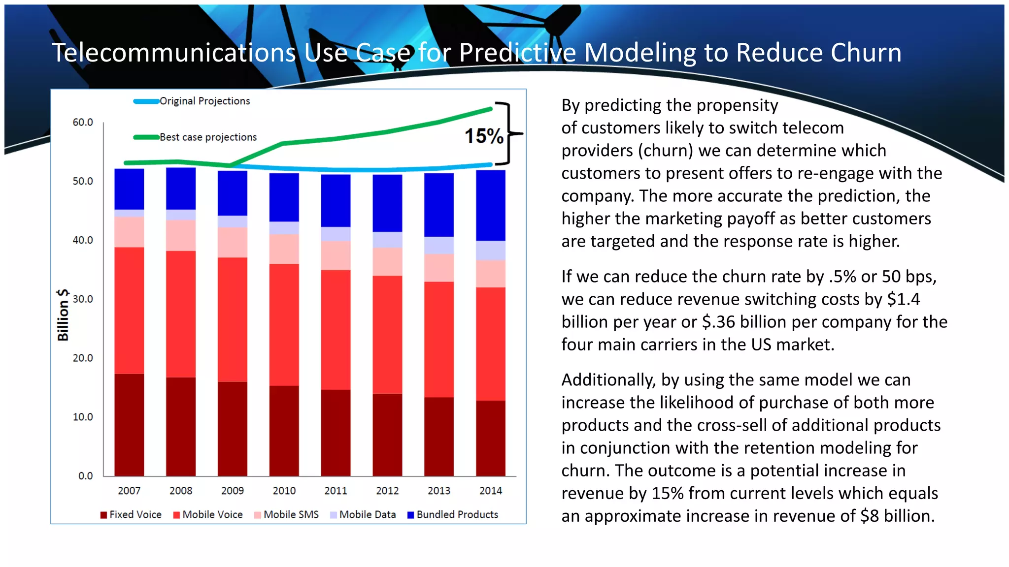
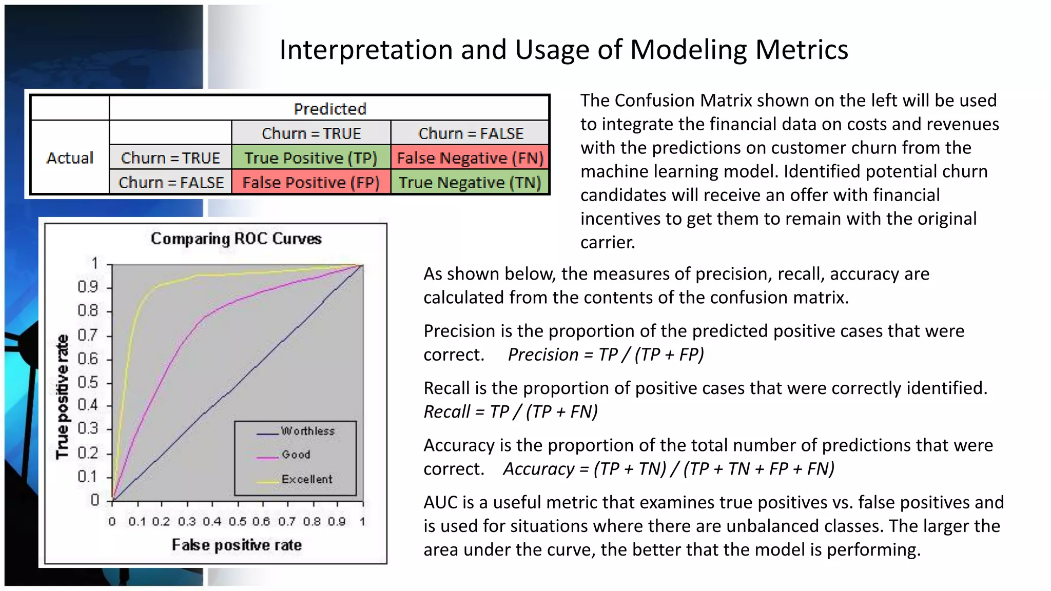
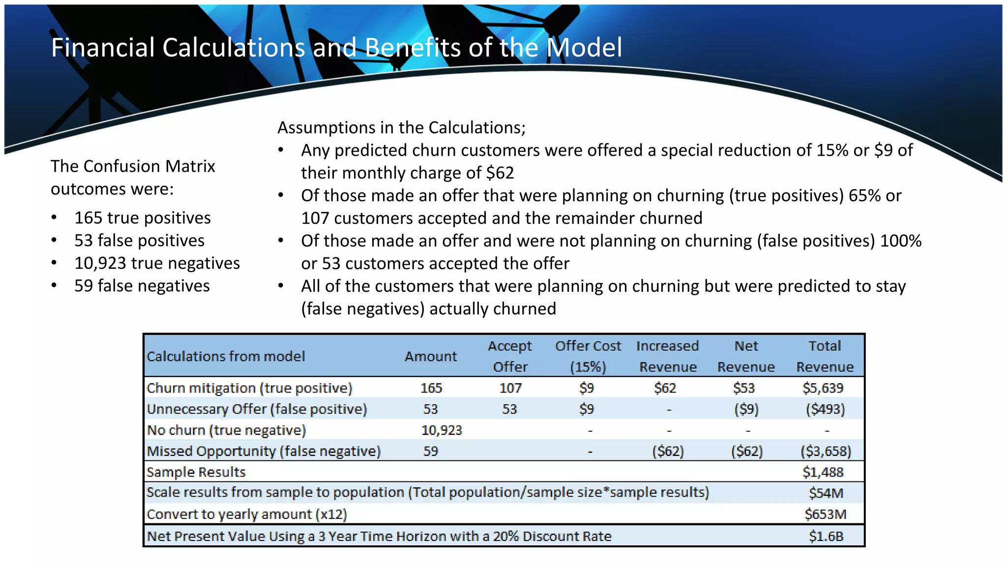
The telecommunications industry faces significant churn, costing companies about $5.7 billion annually due to lost customers, especially as competition increases. Predictive modeling can reduce churn by targeting likely switchers with offers, potentially increasing revenue by $8 billion. Implementing a model that identifies at-risk customers and incentivizes retention could save an estimated $1.6 billion across the industry over three years.

1. Churn in the Telecommunications Industry
“Churn rate (sometimes called attrition rate), in its broadest sense, is a measure of the number of individuals or items
moving out of a collective group over a specific period of time” = Customer Leaving Wikipedia
Churn is a significant problem that costs telecommunications companies billions of dollars through lost revenue. Now
that the market is more mature, the only way for a company to grow is to take their competitors customers. This issue
combined with the greater choice that
consumers have gained means that any
adverse touch point with a consumer can
result in a lost customer.
Typical churn rates for telecom firms are
between 2% and 2.5% per month. The
industry has 400 million customers so this
means a loss of approximately 8 million
customers or a loss of $471 million per
month or $5.7 billion per year in revenue.
In addition, overall average revenue per
unit (ARPU) is declining by 2.7% to 8.7%
per year using traditional marketing
activities.

2. Telecommunications Use Case for Predictive Modeling to Reduce Churn
By predicting the propensity
of customers likely to switch telecom
providers (churn) we can determine which
customers to present offers to re-engage with the
company. The more accurate the prediction, the
higher the marketing payoff as better customers
are targeted and the response rate is higher.
If we can reduce the churn rate by .5% or 50 bps,
we can reduce revenue switching costs by $1.4
billion per year or $.36 billion per company for the
four main carriers in the US market.
Additionally, by using the same model we can
increase the likelihood of purchase of both more
products and the cross-sell of additional products
in conjunction with the retention modeling for
churn. The outcome is a potential increase in
revenue by 15% from current levels which equals
an approximate increase in revenue of $8 billion.

3. Data to be Collected for Building Predictive Models for Churn
The most predictive data for use in the modeling process comes from the actual
transactional and usage data for each individual customer. This data is collected from the
Customer Relationship Management (CRM) application as well as the operational
database which will contain all product, service, purchase and billing data. Additional
data can be acquired through focus groups or 3rd party providers and is less predictive.
Data features are the following
(with relative value – ranked 1-5):
• Purchase history 5
• Products held 5
• Customer Relation Data (which
includes data from all customer
touch points) 5
• Service usage 4
• Billing data 5
Additional data to be acquired:
• Demographic data 3
• Behavioural / psychographic
data 3
• Social values 3

4. Data Sources to be Utilized for Building Predictive Models for Churn
The main data source for this study is the churn dataset
originally from the UCI Machine Learning Repository (converted to MLC++ format1),
which is now included in the package C50 of the R language2. Other data sources include the following industry
reports: Breaking the Back of Customer Churn by Bain & Company, Global Telecommunications Study: Navigating
the Road to 2020 by Ernst & Young, Telecommunications Industry at Cliff’s Edge by McKinsey & Company, and
Churn in the Telecom Industry by NYU Courant & Stern.
The main operational data comes for the UCI
Machine Learning Repository while data on industry
financial metrics, churn rates, acquisition costs,
market sizing and lost revenue is from the industry
reports.
The operational data will be modeled using various
machine learning algorithms and combined with the
financial data and industry data to produce a holistic
view of the financial impact of churn and the
potential benefits from mitigating it.
1http://www.sgi.com/tech/mlc/db/
2http://cran.r-project.org/web/packages/C50

5. Pattern
Evaluation/
Model
Optimization
Data Mining/
Predictive
Modeling
Integrated
and
Preprocessed
Data
Pattern
Information
Knowledge
Data Selection
Data Availability and Priority for Modeling Purposes
Data availability is good for operational data variables but is less so for other types of
data. A huge issue is always data cleansing and dealing with missing variables. Data
integration can be challenging as well.
Data priority generally follows the following process laid-out in the diagram below with
data preprocessing first, followed by data integration, data selection, and then data
evaluation prior to model development / optimization.

6. Model
Lift
Data Transformations for Different Modeling Approaches
Multiple types of predictive models will be
utilized in the modeling process with each model being scored on a separate
test dataset which has not been used to train the models. Both classification and regression models
such as Decision Trees, Random Forests, Neural Networks, Support Vector Machines, Generalized Boosted Models,
Stochastic Gradient Boosting, and Logistic Regression can be implemented and scored against each other.
Standardization is a key data preparation technique if the variables
differ markedly in their magnitude or scale.
Variable reduction is used when dealing with sparse data matrices that
have multiple missing values and when the number of variables is large
– an example is lasso regression.
Dimensionality reduction is used when variables are highly collinear and
when there are many of them – examples include principal components
analysis and factor analysis.
Missing value imputation using regression or statistical approximations
is useful for regression analysis.
Converting from numerical to categorical variables can help to interpret
and visualize the numerical variable, but also can add an additional
feature that could increase the performance of the predictive model by
reducing noise or non-linearity.

7. Interpretation and Usage of Modeling Metrics
The Confusion Matrix shown on the left will be used
to integrate the financial data on costs and revenues
with the predictions on customer churn from the
machine learning model. Identified potential churn
candidates will receive an offer with financial
incentives to get them to remain with the original
carrier.
As shown below, the measures of precision, recall, accuracy are
calculated from the contents of the confusion matrix.
Precision is the proportion of the predicted positive cases that were
correct. Precision = TP / (TP + FP)
Recall is the proportion of positive cases that were correctly identified.
Recall = TP / (TP + FN)
Accuracy is the proportion of the total number of predictions that were
correct. Accuracy = (TP + TN) / (TP + TN + FP + FN)
AUC is a useful metric that examines true positives vs. false positives and
is used for situations where there are unbalanced classes. The larger the
area under the curve, the better that the model is performing.

8. Data Preparation, Pre-processing and Exploration
The dataset was first checked to see if there were any missing
values, correlated features, and variables with near-zero variance. Then the relative
magnitude of the variables was examined to see if the variables required normalization. Since this dataset was
already pre-processed none of these
adjustments were necessary.
Likewise, there was no need for
dimensionality reduction nor variable
reduction.
The next step was to examine the data itself
and see if any characteristics stood out. We
can see right away that thee are some
significant differences in some level of the
features between the customers that
churned and did not churn.
Significant differences were noted in
total_day_minutes, total_day_charge and
all_charge. Customers that churned had
significantly higher charges in all three of
these variables.

9. Exploratory Data Analysis continued
Other features with significant differences between the
customers that churned and those that stayed included the
number of service calls. The histogram on the right shows
the relatively higher proportion of service calls for the
customers that churned.
In fact, customers with four or more customer service calls
churned more than four times as often as the customers
with less than four service calls.
Other interesting observations were that customers with
the International Plan tended to churn more frequently
and customers with the Voice Mail Plan tended to churn
less frequently.
The variables mentioned so far ended up ranking as the
most significant variables in the final version of the model.

10. Model Development and Processing
The dataset was partitioned into training
and test datasets. Next we specified the type of resampling as three separate
10-fold cross-validations. This process was utilized to get the maximum amount of use from the
dataset since it was not that large. In addition, it was noted that the dataset used undersampling3 for the majority
class in order to correct for class imbalances and ensure that the prediction algorithms ran correctly. Such undersampling
needs to be reversed prior to generating any conclusions from the results.
A decision was made to use three distinct types of algorithms to model the data – Random Forests, Generalized Boosted
Models, and Support Vector Machines. The outputs from the final models generated on the training dataset are
specified below.
The best model was the Random Forest Model with an Accuracy Rate of 0.9604, a Precision Rate of 0.9593 and a Recall
Rate of 0.7366. The Out-of-sample-error was only 0.0396 so the model performed very well.
3 https://en.wikipedia.org/wiki/Oversampling_and_undersampling_in_data_analysis

11. Model Results and Evaluation on the Training Dataset
The final metric examined
was Area Under the Curve
(AUC) which was 0.9599 for
the Random Forest Model.
It is apparent from
examining the ROC graph on
the left that the best model
as shown by the highest
curve to the top of the
graph was the Random
Forest Model.
Although the Generalized
Boosted Models were close,
they generated more false
positives and false negatives
than the Random Forest
Model.

12. Outputs From the Test Dataset and Undersampling Correction
After the models were evaluated using three runs of 10 fold
cross-validation on the training dataset, the Random Forests Model emerged as the overall
winner with higher scores in all of the relevant metrics – Precision, Recall, Accuracy, and Area Under the Curve.
To reiterate, cross-validation is a model validation technique for assessing how the results of a statistical analysis
will generalize to an independent data set. It is mainly used in settings where the goal is prediction, and one
wants to estimate how accurately a predictive model will perform in practice.
The next stage was to take the winning model and run it against the test dataset which had not been utilized for
any of the analysis at this point. The outcome from
this final run would then be used to rate how well
the model would perform in a real world scenario
since the data the model was being tested against
was from out-of-sample.
The output from the model was a confusion matrix
that indicated how well the model predicted both
positive and negative outcomes. In order to make
the results comparable with the actual class
composition in the industry, the undersampling for
the majority class was accounted for in this step.
Confusion Matrix

13. Telecom Industry Market Size and Average Financial Metrics
The Telecommunications Industry market size and average financial metrics are listed
below. There are four major carriers in the US market and each of them has approximately
25% or 100M customers of the 400M in the market. The market is saturated and given
that 92% of the US population currently owns a cell phone, the only way for companies to
grow is through acquiring their competitors
customers.
The average monthly revenue per customer
is $62 and companies have gross margins of
55% or $34 per customer.
Monthly loss from churn for each of the
four carriers is approximately $65M.
Finally, acquisition costs are $315 per
customer so it is the best interests of each
carrier to offer a competitive discount in
order to retain their customers.

14. Financial Calculations and Benefits of the Model
The Confusion Matrix
outcomes were:
• 165 true positives
• 53 false positives
• 10,923 true negatives
• 59 false negatives
Assumptions in the Calculations;
• Any predicted churn customers were offered a special reduction of 15% or $9 of
their monthly charge of $62
• Of those made an offer that were planning on churning (true positives) 65% or
107 customers accepted and the remainder churned
• Of those made an offer and were not planning on churning (false positives) 100%
or 53 customers accepted the offer
• All of the customers that were planning on churning but were predicted to stay
(false negatives) actually churned

15. Implications of the Model
Predicting false negative values present the most financial implications to a telecom service provider since this is the
only outcome in which a service provider loses a customer. Some of these financial implications include:
• Revenue loss on the remainder of the customer’s contract
• Costs for acquiring a new customer which includes marketing costs
The aim for each service provider is to maximize their revenues and profits. This can only be achieved if they retain
majority of their customers and prevent customer churn. So, the goal for the model is to maximize the profits by
minimizing the false negative values. The lower the false negative values, the higher will be the profit.
In the model developed and evaluated in this business case, the overall benefits of proactively modeling for churn
and incenting identified customers to stay was $1.6B over a standard 3 year timeframe.
Recommendations
The finished model should be implemented across the industry to score the Telecom company’s customers for the
likelihood of churn. Any identified customers should receive an offer of a 15% rebate for their telecom services for
the next calendar year.
As shown by the selected model enough of these customers will be retained by the offering telecom service
providers such that the total benefits that will accrue across the industry from implementing this strategy will be
approximately $1.6 billion over a standard 3 year timeframe.