The chi-square test is used to determine if experimental data fits the results expected from genetic theory. It involves calculating an expected and observed count for each phenotype, then using a chi-square formula to determine how well the observed fits the expected. The result is compared to critical chi-square values from a table based on degrees of freedom and probability to determine if the null hypothesis should be rejected or failed to be rejected.

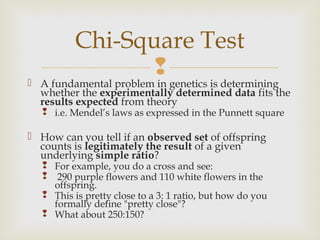
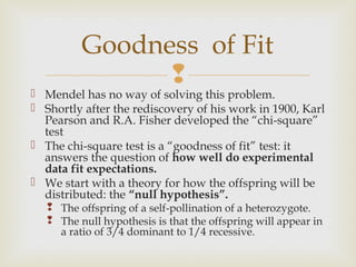
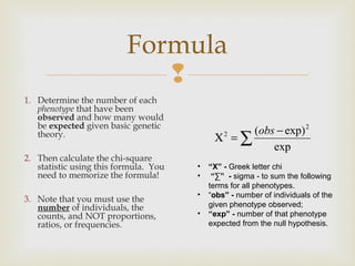
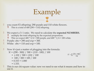
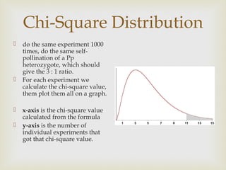
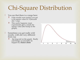
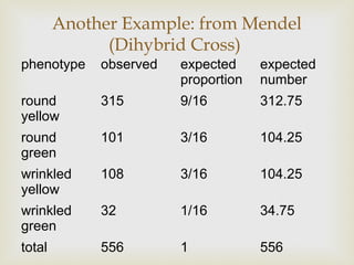
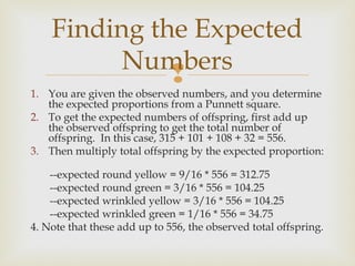
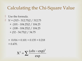
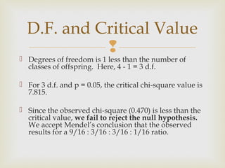
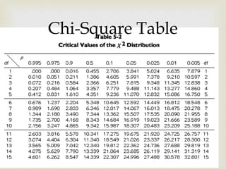
1. “The Goodness Fit” model

2. Chi-Square Test

 A fundamental problem in genetics is determining
whether the experimentally determined data fits the
results expected from theory
 i.e. Mendel’s laws as expressed in the Punnett square
 How can you tell if an observed set of offspring
counts is legitimately the result of a given
underlying simple ratio?
 For example, you do a cross and see:
 290 purple flowers and 110 white flowers in the
offspring.
 This is pretty close to a 3: 1 ratio, but how do you
formally define "pretty close"?
 What about 250:150?

3. Goodness of Fit

 Mendel has no way of solving this problem.
 Shortly after the rediscovery of his work in 1900, Karl
Pearson and R.A. Fisher developed the “chi-square”
test
 The chi-square test is a “goodness of fit” test: it
answers the question of how well do experimental
data fit expectations.
 We start with a theory for how the offspring will be
distributed: the “null hypothesis”.
 The offspring of a self-pollination of a heterozygote.
 The null hypothesis is that the offspring will appear in
a ratio of 3/4 dominant to 1/4 recessive.

4. Formula

1. Determine the number of each
phenotype that have been
observed and how many would
be expected given basic genetic
(obs − exp) 2
theory. Χ2 = ∑
exp
2. Then calculate the chi-square
statistic using this formula. You • “Χ” - Greek letter chi
need to memorize the formula! • “∑” - sigma - to sum the following
terms for all phenotypes.
• “obs” - number of individuals of the
3. Note that you must use the
number of individuals, the given phenotype observed;
counts, and NOT proportions, • “exp” - number of that phenotype
ratios, or frequencies. expected from the null hypothesis.

5. Example

 you count F2 offspring: 290 purple and 110 white flowers.
 This is a total of 400 (290 + 110) offspring.
 We expect a 3: 1 ratio. We need to calculate the expected NUMBERS.
 multiply the total offspring by the expected proportions.
 This we expect 400 * 3/4 = 300 purple, and 400 * 1/4 = 100 white.
 Purple: obs = 290 and exp = 300.
 White: obs = 110 and exp = 100.
 Now it's just a matter of plugging into the formula:
Χ2 = (290 - 300)2 / 300 + (110 - 100)2 / 100
= (-10)2 / 300 + (10)2 / 100
= 100 / 300 + 100 / 100
= 0.333 + 1.000
= 1.333.
 This is our chi-square value: now we need to see what it means and how to
use it.

6. Chi-Square Distribution
 do the same experiment 1000
times, do the same self-
pollination of a Pp
heterozygote, which should
give the 3 : 1 ratio.
 For each experiment we
calculate the chi-square value,
them plot them all on a graph.
 x-axis is the chi-square value
calculated from the formula
 y-axis is the number of
individual experiments that
got that chi-square value.

7. Chi-Square Distribution
 You see that there is a range here:
 if the results were perfect you get
a chi-square value of 0 (because
obs = exp).
 This rarely happens: most
experiments give a small chi-
square value (the hump in the
graph).
 Sometimes you get really wild
results, with obs very different
from exp
 the long tail on the graph. Really
odd things occasionally do
happen by chance alone

8. The Critical Question

result?


How do you tell a really odd but correct result from a WRONG
occasionally very skewed distributions of data occur even though you
performed the experiment correctly (correct theory)
 Never for certain that a given result is “wrong”,
 determine whether a given result is likely or unlikely.
 2 ways of getting a high chi-square value: ( statistics is never able
to discriminate between true and false with 100% certainty)
 an unusual result from the correct theory,
 or a result from the wrong theory.
 Does your 290: 110 offspring ratio really fit a 3/4 : 1/4 ratio or was
it the result of a mistake or accident?
 You can’t be certain, but you can at least determine whether your result
is REASONABLE

9. Reasonable

 subjective and arbitrary.
 A result is said to not differ significantly from expectations, if the
difference between the observed results and the expected results is
small enough that it would be seen at least 1 time in 20 over
thousands of experiments
 For technical reasons, we use “fail to reject” instead of “accept”.
 Probability value p = 0.05, because 1/20 = 0.05.

10. Degrees of Freedom

 the number of independent random variables
involved.
 Degrees of freedom is simply the number of classes
of offspring minus 1.
 For our example, there are 2 classes of offspring:
purple and white. Thus, degrees of freedom (d.f.) =
2 -1 = 1.

11. Critical Chi-Square


Sorted by degrees of freedom
and probability levels. Be sure
to use p = 0.05.
 If chi-square value is greater
than the critical value from the
table, you “reject the null
hypothesis”.
 If chi-square value is less than
the critical value, you “fail to
reject” the null hypothesis

12. Using the Table

 290 purple to 110 white,
 chi-square value of 1.333
 1 degree of freedom.
 1 d.f. is the first row
 p = 0.05 is the sixth column
 critical chi-square value, 3.841.
 chi-square, 1.333, is less than
the critical value, 3.841, we “fail
to reject” the null hypothesis.
 Thus, an observed ratio of 290
purple to 110 white is a good fit
to a 3/4 to 1/4 ratio.

13. Another Example: from Mendel
(Dihybrid Cross)
phenotype observed expected expected
proportion number
round 315
yellow
round 101
green
wrinkled 108
yellow
wrinkled 32
green
total 556

14. Another Example: from Mendel
(Dihybrid Cross)
phenotype observed expected expected
proportion number
round 315 9/16
yellow
round 101 3/16
green
wrinkled 108 3/16
yellow
wrinkled 32 1/16
green
total 556 1

15. Another Example: from Mendel
(Dihybrid Cross)
phenotype observed expected expected
proportion number
round 315 9/16 312.75
yellow
round 101 3/16 104.25
green
wrinkled 108 3/16 104.25
yellow
wrinkled 32 1/16 34.75
green
total 556 1 556

16. Finding the Expected
Numbers

1. You are given the observed numbers, and you determine
the expected proportions from a Punnett square.
2. To get the expected numbers of offspring, first add up
the observed offspring to get the total number of
offspring. In this case, 315 + 101 + 108 + 32 = 556.
3. Then multiply total offspring by the expected proportion:
--expected round yellow = 9/16 * 556 = 312.75
--expected round green = 3/16 * 556 = 104.25
--expected wrinkled yellow = 3/16 * 556 = 104.25
--expected wrinkled green = 1/16 * 556 = 34.75
4. Note that these add up to 556, the observed total offspring.

17. Calculating the Chi-Square Value
 Use the formula.
 X2 = (315 - 312.75)2 / 312.75
+ (101 - 104.25)2 / 104.25
+ (108 - 104.25)2 / 104.25
+ (32 - 34.75)2 / 34.75
= 0.016 + 0.101 + 0.135 + 0.218
= 0.470.
(obs − exp) 2
Χ =∑
2
exp

18. D.F. and Critical Value

 Degrees of freedom is 1 less than the number of
classes of offspring. Here, 4 - 1 = 3 d.f.
 For 3 d.f. and p = 0.05, the critical chi-square value is
7.815.
 Since the observed chi-square (0.470) is less than the
critical value, we fail to reject the null hypothesis.
We accept Mendel’s conclusion that the observed
results for a 9/16 : 3/16 : 3/16 : 1/16 ratio.

19. Chi-Square Table
