CHAPTER 5:
DISCRETE FOURIERTRANSFORM
(DFT)
Lecture 9: DFT and Inverse DFT
Lecture 10: Fast Fourier Transform (FFT)
Duration: 4 hrs
2.
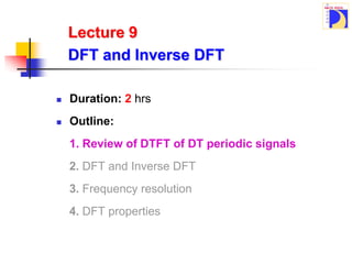
Lecture 9
DFT andInverse DFT
Duration: 2 hrs
Outline:
1. Review of DTFT of DT periodic signals
2. DFT and Inverse DFT
3. Frequency resolution
4. DFT properties
3.
Procedure to calculateDTFT of
periodic signals
Step 1:
Start with x0(n) – one period of x(n), with zero everywhere else
Step 2:
Find the DTFT X0(Ω) of the signal x0[n] above
Step 3:
Find X0(Ω) at N equally spacing frequency points X0(k2π/N)
Step 4:
Obtain the DTFT of x(n):
k N
k
N
k
X
N
X )
2
(
)
2
(
2
)
( 0
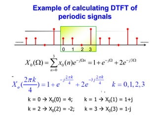
4.
Example of calculatingDTFT of
periodic signals
3
3
0
0
0 2
1
)
(
)
( j
j
n
n
j
e
e
e
n
x
X
k = 0 X0(0) = 4; k = 1 X0(1) = 1+j
k = 2 X0(2) = -2; k = 3 X0(3) = 1-j
0 1 2 3
Lecture 9
DFT andInverse DFT
Duration: 2 hrs
Outline:
1. Review of DTFT of DT periodic signals
2. DFT and Inverse DFT
3. Frequency resolution
4. Applications
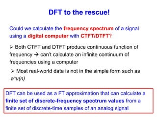
7.
DFT to therescue!
Both CTFT and DTFT produce continuous function of
frequency can’t calculate an infinite continuum of
frequencies using a computer
Most real-world data is not in the simple form such as
anu(n)
DFT can be used as a FT approximation that can calculate a
finite set of discrete-frequency spectrum values from a
finite set of discrete-time samples of an analog signal
Could we calculate the frequency spectrum of a signal
using a digital computer with CTFT/DTFT?
8.
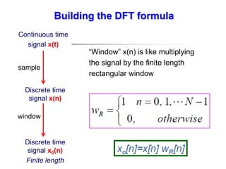
Building the DFTformula
“Window” x(n) is like multiplying
the signal by the finite length
rectangular window
Discrete time
signal x(n)
Continuous time
signal x(t)
Discrete time
signal x0(n)
Finite length
sample
window
9.
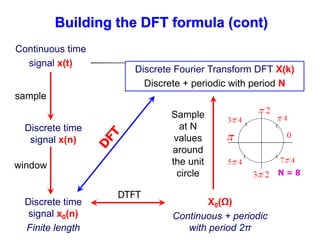
Building the DFTformula (cont)
DTFT
1
0
0
0
0 ]
[
]
[
)
(
N
n
n
j
n
n
j
e
n
x
e
n
x
X
Discrete time
signal x(n)
Continuous time
signal x(t)
Discrete time
signal x0(n)
Finite length
sample
window
10.
Building the DFTformula (cont)
Discrete time
signal x(n)
Discrete time
signal x0(n)
Finite length
sample
window
DTFT
Sample
at N
values
around
the unit
circle
Discrete Fourier Transform DFT X(k)
Discrete + periodic with period N
X0(Ω)
Continuous + periodic
with period 2π
N = 8
Continuous time
signal x(t)
11.
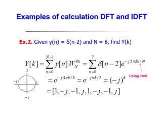
DFT and inverseDFT formulas
N
2
j
N e
W
Notation:
You only have to store N points
12.
k = 0 X(k) = X(0) = N
k ≠ 0 X(k) = 0
Ex.1. Find the DFT of x(n) = 1, n = 0, 1, 2, …, (N-1)
Examples of calculation DFT and IDFT
13.
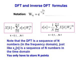
Ex.2. Given y(n)= δ(n-2) and N = 8, find Y(k)
Examples of calculation DFT and IDFT
14.
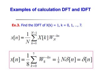
Ex.3. Find theIDFT of X(k) = 1, k = 0, 1, …, 7.
Examples of calculation DFT and IDFT
15.
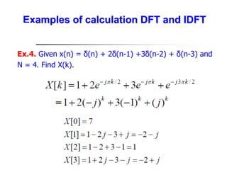
Examples of calculationDFT and IDFT
Ex.4. Given x(n) = δ(n) + 2δ(n-1) +3δ(n-2) + δ(n-3) and
N = 4. Find X(k).
Lecture 9
DFT andInverse DFT
Duration: 2 hrs
Outline:
1. Review of DTFT of DT periodic signals
2. DFT and Inverse DFT
3. Frequency resolution
4. DFT properties
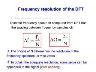
18.
Discrete frequency spectrumcomputed from DFT has
the spacing between frequency samples of:
N
f
f s
N
2
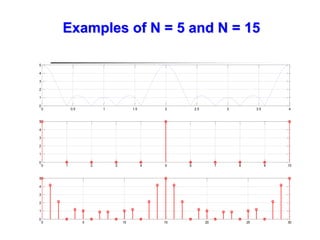
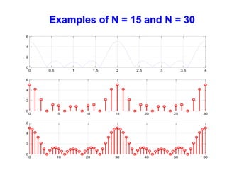
The choice of N determines the resolution of the
frequency spectrum, or vice-versa
To obtain the adequate resolution, some zeros can be
appended to the signal (zero padding)
Frequency resolution of the DFT
Lecture 9
DFT andInverse DFT
Duration: 2 hrs
Outline:
1. Review of DTFT of DT periodic signals
2. DFT and Inverse DFT
3. Frequency resolution
4. DFT properties
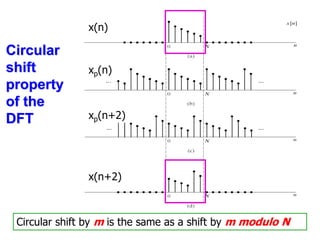
22.
Circular shift propertyof the DFT
x(n) is one period of signal xp(n)
x(n)
Finite length
xp(n)
Infinite length,
periodic
N periodic extension
truncate
]
k
[
X
W
]
m
n
[
x km
DFT
Recall linear convolution
N1: the non-zero length of x1(n); N2: the non-zero
length of x2(n); Ny = N1 + N2 -1
The shift operation is the regular shift
The flip operation is the regular flip
p
p
n
x
p
x
n
x
n
x
n
y ]
[
]
[
]
[
*
]
[
]
[ 2
1
2
1
25.
Circular convolution ofthe DFT
The non-zero length of x1(n), x2(n) and y(n) can be no
longer than N
The shift operation is circular shift
The flip operation is circular flip
1
0
mod
2
1
2
1 ]
[
]
[
]
[
]
[
]
[
N
p
N
p
n
x
p
x
n
x
n
x
n
y
26.
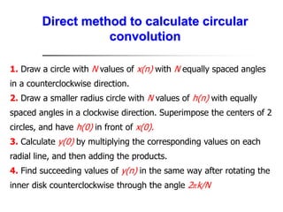
Direct method tocalculate circular
convolution
1. Draw a circle with N values of x(n) with N equally spaced angles
in a counterclockwise direction.
2. Draw a smaller radius circle with N values of h(n) with equally
spaced angles in a clockwise direction. Superimpose the centers of 2
circles, and have h(0) in front of x(0).
3. Calculate y(0) by multiplying the corresponding values on each
radial line, and then adding the products.
4. Find succeeding values of y(n) in the same way after rotating the
inner disk counterclockwise through the angle 2πk/N
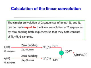
Calculation of thelinear convolution
x1(n)
N1 samples
x2(n)
N2 samples
x’1(n)
x’2(n)
Zero padding
(N2-1) zeros
IDFT
x1(n)*x2(n)
Zero padding
(N1-1) zeros
DFT
DFT
The circular convolution of 2 sequences of length N1 and N2
can be made equal to the linear convolution of 2 sequences
by zero padding both sequences so that they both consists
of N1+N2-1 samples.
Prob.1
Compute the DFTwith N time samples:
1
N
n
0
odd
n
0
even
n
1
]
n
[
x
)
c
(
]}
N
n
[
u
]
n
[
u
{
a
]
n
[
x
)
b
(
]
n
[
]
n
[
x
)
a
(
n
HW
33.
Prob.2
Given the twofour-point sequences:
HW
x(n) = [ 1 0.75 0.5 0.25 ]
y(n) = [ 0.75 0.5 0.25 1]
Express the DFT Y(k) in terms of the DFT X(k)
34.
Prob.3
Given signals belowand their DFT-5
HW
]
n
[
]
n
[
s
)
c
(
]
1
n
[
]
n
[
x
)
b
(
]
4
n
[
4
]
3
n
[
3
]
2
n
[
2
]
1
n
[
]
n
[
x
)
a
(
2
1
1. Find y[n] so that Y[k] = X1[k].X2[k]
2. Does x3[n] exist, if S[k] = X1[k].X3[k]?
35.
Prob.4 Given x(n)and its 8-point DFT, X(k)
HW
7
n
4
,
0
3
n
0
,
1
]
n
[
x
Express the DFTs of the signals below in terms of X(k).
7
n
6
,
0
5
n
2
,
1
1
n
0
,
0
]
n
[
x
)
b
(
7
n
5
,
1
4
n
1
,
0
0
n
,
1
]
n
[
x
)
a
(
2
1
36.
Prob.5 The 8-pointDFTs of x(n) and h(n) are:
X(k) = [0, -j0.707, -j, -j0.707, 0, j0.707, j, j0.707]
and
H(k) = [3, 2.414, 1, -0.414, -1, -0.414, 1, 2.414]
HW
Find the value of y(2), where y(n) is the circular convolution
of x(n) and h(n).
37.
Lecture 10
Fast FourierTransform (FFT)
Duration: 2 hrs
Outline:
1. What is FFT?
2. The decomposition-in-time Fast Fourier
Transform algorithm
38.
DFT plays animportant role in the analysis, design and
implementation of the DT signal processing algorithms and
systems.
Major reason: existence of efficient algorithms for computing
DFT called FFT
N
2
j
N e
W
1
N
n
0
W
]
k
[
X
N
1
]
n
[
x
1
N
k
0
W
]
n
[
x
]
k
[
X
1
N
0
n
nk
N
1
N
0
n
nk
N
Recall DFT and IDFT definition
39.
1
N
k
0
W
]
n
[
x
]
k
[
X
1
N
0
n
nk
N
Thedirect computation of the DFT requires:
1. N complex multiplications for each of k
2. N2 complex multiplications for all N points of X(k)
3. (N-1) complex summations for each of k
4. N(N-1) complex summations for all N points of X(k)
FFT optimize computational processes (1) & (2) in different
algorithms
Direct computation of the DFT
40.
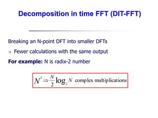
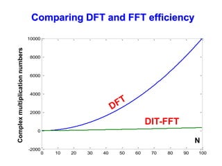
Breaking an N-pointDFT into smaller DFTs
Fewer calculations with the same output
For example: N is radix-2 number
tions
multiplica
complex
2
log2
2
N
N
N
Decomposition in time FFT (DIT-FFT)
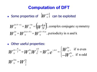
Some propertiesof can be exploited
Other useful properties:
W
nk
N
k
and
n
in
y
periodicit
,
symmetry
conjugate
complex
,
)
(
)
(
*
)
(
W
W
W
W
W
W
n
N
k
N
N
n
k
N
kn
N
kn
N
n
N
k
N
kn
N
W
W
W
W
e
W
W
W
W
kn
N
kn
N
kn
N
kn
N
jn
kn
N
nN
N
kn
N
n
N
k
N
2
2
2
)
2
(
odd
n
if
,
even
n
if
,
Computation of DFT
43.
Lecture 10
Fast FourierTransform (FFT)
Duration: 2 hrs
Outline:
1. What is FFT?
2. The decomposition-in-time Fast Fourier
Transform algorithm
44.
G(k) isN/2 points DFT of the even numbered data: x(0),
x(2), x(4), …., x(N-2).
H(k) is the N/2 points DFT of the odd numbered data:
x(1), x(3), …, x(N-1).
even odd
[ ] [ ] [ ]
kn kn
n n
X k x n W x n W
DIT-FFT with N as a 2-radix number
45.
2 2
1 1
2(2 1)
0 0
[ ] [2 ] [2 1]
N N
mk k m
m m
X k x m W x m W
2 2
1 1
2 2
0 0
[2 ]( ) [2 1]( )
N N
mk k mk
m m
x m W W x m W
=
2
/
N
)
2
/
N
/(
2
j
2
N
/
2
j
2
N W
e
e
W
G(k) and H(k) are of length N/2; X(k) is of length N
G(k)=G(k+N/2) and H(k)=H(k+N/2)
1
N
,...,
1
,
0
k
),
k
(
H
)
k
(
G
)
k
(
X W
k
N
DIT-FFT (cont)
Now the overallcomputation is reduced to:
tions
multiplica
complex
2
log2
2
N
N
N
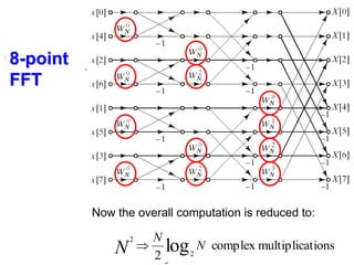
8-point
FFT
50.
Prob.6
(a) Draw aneight-point DIT FFT signal-flow diagram, and use
it to solve for the DFT of the sequence x(n)
x(n) = (0.5) n [u(n) – u(n-8)]
HW
(b) Use Matlab (fft) to confirm the result of part (a)

![Procedure to calculate DTFT of
periodic signals
Step 1:
Start with x0(n) – one period of x(n), with zero everywhere else
Step 2:
Find the DTFT X0(Ω) of the signal x0[n] above
Step 3:
Find X0(Ω) at N equally spacing frequency points X0(k2π/N)
Step 4:
Obtain the DTFT of x(n):
k N
k
N
k
X
N
X )
2
(
)
2
(
2
)
( 0
](https://image.slidesharecdn.com/chapter5discretefouriertransform-251214075349-ae81f125/85/Chapter5_DISCRETEr-FOURIER-TRANSFORM-pdf-3-320.jpg)
![Building the DFT formula (cont)
DTFT
1
0
0
0
0 ]
[
]
[
)
(
N
n
n
j
n
n
j
e
n
x
e
n
x
X
Discrete time
signal x(n)
Continuous time
signal x(t)
Discrete time
signal x0(n)
Finite length
sample
window](https://image.slidesharecdn.com/chapter5discretefouriertransform-251214075349-ae81f125/85/Chapter5_DISCRETEr-FOURIER-TRANSFORM-pdf-9-320.jpg)

![ x = [1 2 3 1];
>> X = fft(x)
X = 7.0000 -2.0000 - 1.0000i 1.0000 -2.0000
+ 1.0000i
7.0000 1.7071 - 5.1213i -2.0000 - 1.0000i 0.2929 +
0.8787i
Columns 5 through 8
1.0000 0.2929 - 0.8787i -2.0000 + 1.0000i 1.7071
+ 5.1213i](https://image.slidesharecdn.com/chapter5discretefouriertransform-251214075349-ae81f125/85/Chapter5_DISCRETEr-FOURIER-TRANSFORM-pdf-16-320.jpg)
![Circular shift property of the DFT
x(n) is one period of signal xp(n)
x(n)
Finite length
xp(n)
Infinite length,
periodic
N periodic extension
truncate
]
k
[
X
W
]
m
n
[
x km
DFT
](https://image.slidesharecdn.com/chapter5discretefouriertransform-251214075349-ae81f125/85/Chapter5_DISCRETEr-FOURIER-TRANSFORM-pdf-22-320.jpg)
![Recall linear convolution
N1: the non-zero length of x1(n); N2: the non-zero
length of x2(n); Ny = N1 + N2 -1
The shift operation is the regular shift
The flip operation is the regular flip
p
p
n
x
p
x
n
x
n
x
n
y ]
[
]
[
]
[
*
]
[
]
[ 2
1
2
1](https://image.slidesharecdn.com/chapter5discretefouriertransform-251214075349-ae81f125/85/Chapter5_DISCRETEr-FOURIER-TRANSFORM-pdf-24-320.jpg)
![Circular convolution of the DFT
The non-zero length of x1(n), x2(n) and y(n) can be no
longer than N
The shift operation is circular shift
The flip operation is circular flip
1
0
mod
2
1
2
1 ]
[
]
[
]
[
]
[
]
[
N
p
N
p
n
x
p
x
n
x
n
x
n
y](https://image.slidesharecdn.com/chapter5discretefouriertransform-251214075349-ae81f125/85/Chapter5_DISCRETEr-FOURIER-TRANSFORM-pdf-25-320.jpg)
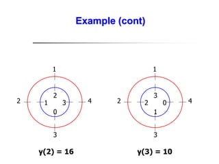
![Example to calculate circular convolution
Evaluate the circular convolution, y(n) of 2 signals:
x1(n) = [ 1 2 3 4 ]; x2(n) = [ 0 1 2 3 ]
1
2
3
4
0
1
2
3
y(0) = 16
1
2
3
4
1
2
3
0
y(1) = 18](https://image.slidesharecdn.com/chapter5discretefouriertransform-251214075349-ae81f125/85/Chapter5_DISCRETEr-FOURIER-TRANSFORM-pdf-27-320.jpg)
![Another method to calculate circular
convolution
x1(n)
x2(n)
X1(k)
X2(k)
DFT
DFT
IDFT y(n)
Ex. x1(n) = [ 1 2 3 4 ]; x2(n) = [ 0 1 2 3 ]
X1(k) = [ 10, -2+j2, -2, -2-j2 ];
X2(k) = [ 6, -2+j2, -2, -2-j2 ];
Y(k) = X1(k).X2(k) = [ 60, -j8, 4, j8 ]
y(n) = [ 16, 18, 16, 10 ]](https://image.slidesharecdn.com/chapter5discretefouriertransform-251214075349-ae81f125/85/Chapter5_DISCRETEr-FOURIER-TRANSFORM-pdf-29-320.jpg)
![x1(n) = [ 1 2 3 4 ]; x2(n) = [ 0 1 2 3 ]
x’1(n) = [ 1 2 3 4 0 0 0 ]; x’2(n) = [ 0 1 2 3 0 0 0 ]
X’1(k) = [ 10, -2.0245-j6.2240, 0.3460+j2.4791, 0.1784-
j2.4220, 0.1784+j2.4220, 0.3460-j2.4791, -2.0245-j6.2240 ];
X’2(k) = [ 6, -2.5245-j4.0333, -0.1540+j2.2383, -0.3216-
j1.7950, -0.3216+j1.7950, -0.1540-j2.2383, -2.5245+j4.0333];
Y’(k) = [ 60, -19.9928+j23.8775, -5.6024+j0.3927, -5.8342-
j0.8644, -4.4049+j0.4585, -5.6024-j0.3927, -19.9928
+j23.8775 ]
IDFT{Y’(k)} = y’(n) = [ 0 1 4 10 16 17 12 ]
Example of calculation the linear convolution](https://image.slidesharecdn.com/chapter5discretefouriertransform-251214075349-ae81f125/85/Chapter5_DISCRETEr-FOURIER-TRANSFORM-pdf-31-320.jpg)
![Prob.1
Compute the DFT with N time samples:
1
N
n
0
odd
n
0
even
n
1
]
n
[
x
)
c
(
]}
N
n
[
u
]
n
[
u
{
a
]
n
[
x
)
b
(
]
n
[
]
n
[
x
)
a
(
n
HW](https://image.slidesharecdn.com/chapter5discretefouriertransform-251214075349-ae81f125/85/Chapter5_DISCRETEr-FOURIER-TRANSFORM-pdf-32-320.jpg)
![Prob.2
Given the two four-point sequences:
HW
x(n) = [ 1 0.75 0.5 0.25 ]
y(n) = [ 0.75 0.5 0.25 1]
Express the DFT Y(k) in terms of the DFT X(k)](https://image.slidesharecdn.com/chapter5discretefouriertransform-251214075349-ae81f125/85/Chapter5_DISCRETEr-FOURIER-TRANSFORM-pdf-33-320.jpg)
![Prob.3
Given signals below and their DFT-5
HW
]
n
[
]
n
[
s
)
c
(
]
1
n
[
]
n
[
x
)
b
(
]
4
n
[
4
]
3
n
[
3
]
2
n
[
2
]
1
n
[
]
n
[
x
)
a
(
2
1
1. Find y[n] so that Y[k] = X1[k].X2[k]
2. Does x3[n] exist, if S[k] = X1[k].X3[k]?](https://image.slidesharecdn.com/chapter5discretefouriertransform-251214075349-ae81f125/85/Chapter5_DISCRETEr-FOURIER-TRANSFORM-pdf-34-320.jpg)
![Prob.4 Given x(n) and its 8-point DFT, X(k)
HW
7
n
4
,
0
3
n
0
,
1
]
n
[
x
Express the DFTs of the signals below in terms of X(k).
7
n
6
,
0
5
n
2
,
1
1
n
0
,
0
]
n
[
x
)
b
(
7
n
5
,
1
4
n
1
,
0
0
n
,
1
]
n
[
x
)
a
(
2
1](https://image.slidesharecdn.com/chapter5discretefouriertransform-251214075349-ae81f125/85/Chapter5_DISCRETEr-FOURIER-TRANSFORM-pdf-35-320.jpg)
![Prob.5 The 8-point DFTs of x(n) and h(n) are:
X(k) = [0, -j0.707, -j, -j0.707, 0, j0.707, j, j0.707]
and
H(k) = [3, 2.414, 1, -0.414, -1, -0.414, 1, 2.414]
HW
Find the value of y(2), where y(n) is the circular convolution
of x(n) and h(n).](https://image.slidesharecdn.com/chapter5discretefouriertransform-251214075349-ae81f125/85/Chapter5_DISCRETEr-FOURIER-TRANSFORM-pdf-36-320.jpg)
![DFT plays an important role in the analysis, design and
implementation of the DT signal processing algorithms and
systems.
Major reason: existence of efficient algorithms for computing
DFT called FFT
N
2
j
N e
W
1
N
n
0
W
]
k
[
X
N
1
]
n
[
x
1
N
k
0
W
]
n
[
x
]
k
[
X
1
N
0
n
nk
N
1
N
0
n
nk
N
Recall DFT and IDFT definition](https://image.slidesharecdn.com/chapter5discretefouriertransform-251214075349-ae81f125/85/Chapter5_DISCRETEr-FOURIER-TRANSFORM-pdf-38-320.jpg)
![1
N
k
0
W
]
n
[
x
]
k
[
X
1
N
0
n
nk
N
The direct computation of the DFT requires:
1. N complex multiplications for each of k
2. N2 complex multiplications for all N points of X(k)
3. (N-1) complex summations for each of k
4. N(N-1) complex summations for all N points of X(k)
FFT optimize computational processes (1) & (2) in different
algorithms
Direct computation of the DFT](https://image.slidesharecdn.com/chapter5discretefouriertransform-251214075349-ae81f125/85/Chapter5_DISCRETEr-FOURIER-TRANSFORM-pdf-39-320.jpg)
![ G(k) is N/2 points DFT of the even numbered data: x(0),
x(2), x(4), …., x(N-2).
H(k) is the N/2 points DFT of the odd numbered data:
x(1), x(3), …, x(N-1).
even odd
[ ] [ ] [ ]
kn kn
n n
X k x n W x n W
DIT-FFT with N as a 2-radix number](https://image.slidesharecdn.com/chapter5discretefouriertransform-251214075349-ae81f125/85/Chapter5_DISCRETEr-FOURIER-TRANSFORM-pdf-44-320.jpg)
![2 2
1 1
2 (2 1)
0 0
[ ] [2 ] [2 1]
N N
mk k m
m m
X k x m W x m W
2 2
1 1
2 2
0 0
[2 ]( ) [2 1]( )
N N
mk k mk
m m
x m W W x m W
=
2
/
N
)
2
/
N
/(
2
j
2
N
/
2
j
2
N W
e
e
W
G(k) and H(k) are of length N/2; X(k) is of length N
G(k)=G(k+N/2) and H(k)=H(k+N/2)
1
N
,...,
1
,
0
k
),
k
(
H
)
k
(
G
)
k
(
X W
k
N
DIT-FFT (cont)](https://image.slidesharecdn.com/chapter5discretefouriertransform-251214075349-ae81f125/85/Chapter5_DISCRETEr-FOURIER-TRANSFORM-pdf-45-320.jpg)
![]
3
[
H
W
]
3
[
G
]
7
[
X
]
2
[
H
W
]
2
[
G
]
6
[
X
]
1
[
H
W
]
1
[
G
]
5
[
X
]
0
[
H
W
]
0
[
G
]
4
[
X
]
3
[
H
W
]
3
[
G
]
3
[
X
]
2
[
H
W
]
2
[
G
]
2
[
X
]
1
[
H
W
]
1
[
G
]
1
[
X
]
0
[
H
W
]
0
[
G
]
0
[
X
7
8
6
8
5
8
4
8
3
8
2
8
1
8
0
8
tions
multiplica
complex
2
2
2
2
2
2
2
2
N
N
N
N N
N
DFT N = 4
DFT N = 4
The new computation counts are reduced
8-point FFT
4
8
4
8 ]
[
]
[
]
[ k
H
W
k
G
k
X k
](https://image.slidesharecdn.com/chapter5discretefouriertransform-251214075349-ae81f125/85/Chapter5_DISCRETEr-FOURIER-TRANSFORM-pdf-46-320.jpg)
![0
W
0
W
W4
W2
W0
W0
W6
W6
W2
W4
DFT N = 2
DFT N = 2
DFT N = 2
DFT N = 2
G[0]
G[1]
G[2]
G[3]
H[0]
H[1]
H[2]
H[3]
8-point
FFT
(cont)](https://image.slidesharecdn.com/chapter5discretefouriertransform-251214075349-ae81f125/85/Chapter5_DISCRETEr-FOURIER-TRANSFORM-pdf-47-320.jpg)
![Prob.6
(a) Draw an eight-point DIT FFT signal-flow diagram, and use
it to solve for the DFT of the sequence x(n)
x(n) = (0.5) n [u(n) – u(n-8)]
HW
(b) Use Matlab (fft) to confirm the result of part (a)](https://image.slidesharecdn.com/chapter5discretefouriertransform-251214075349-ae81f125/85/Chapter5_DISCRETEr-FOURIER-TRANSFORM-pdf-50-320.jpg)