Download as PDF, PPTX
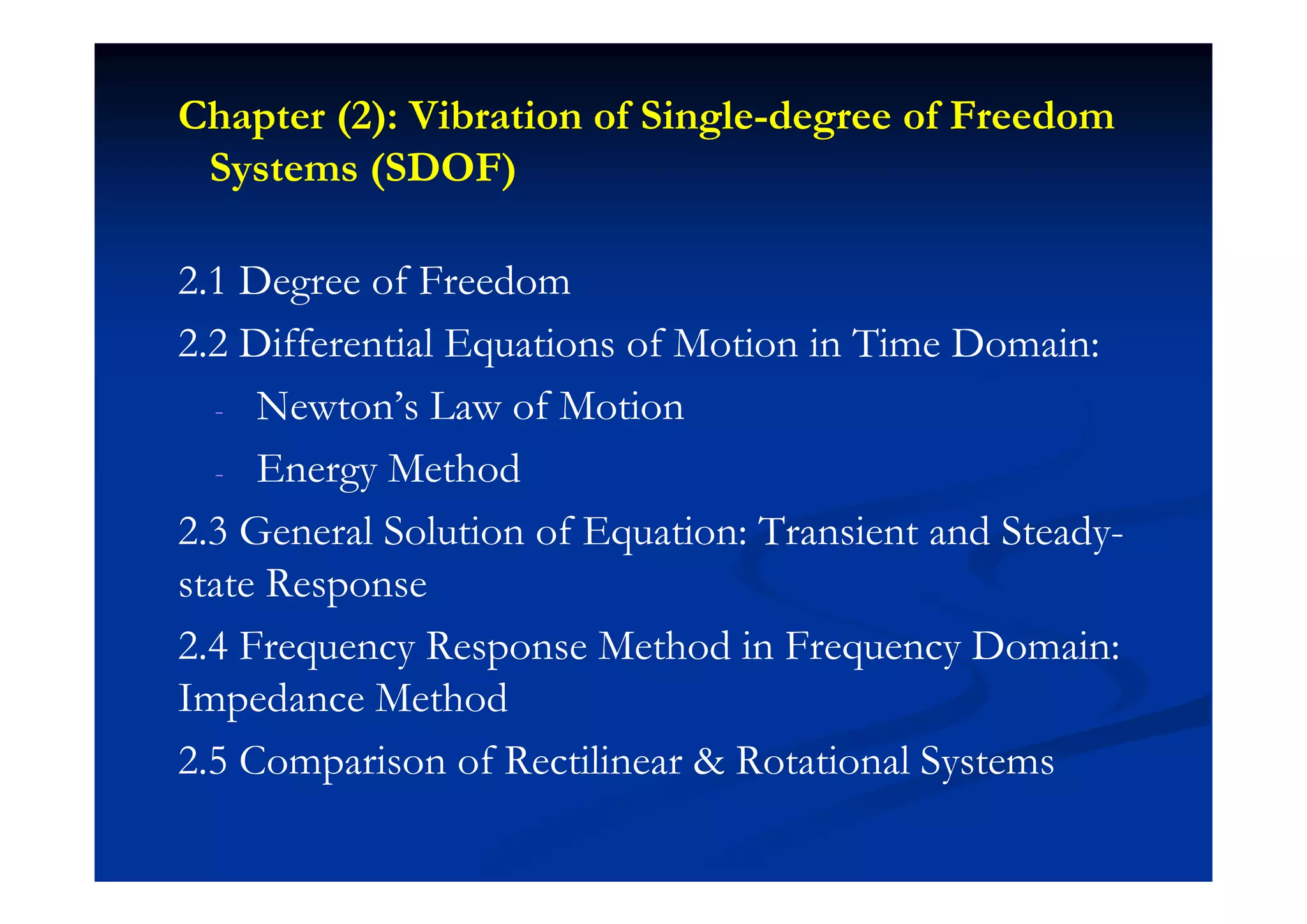
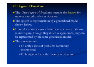
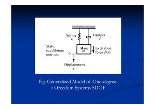
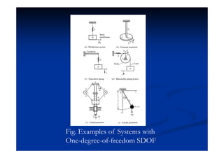
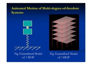
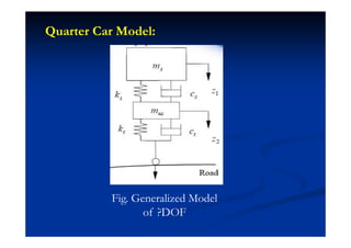
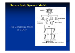
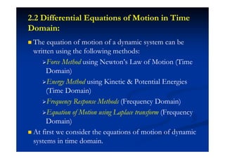
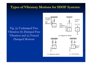
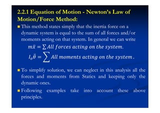
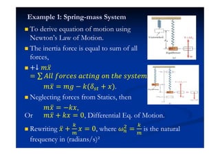
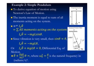
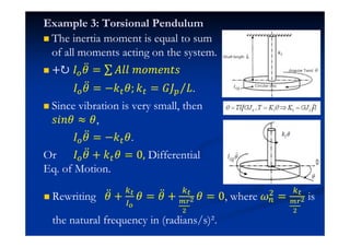
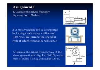
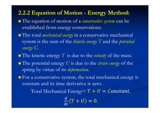
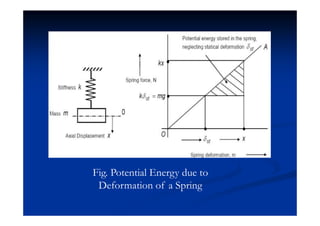
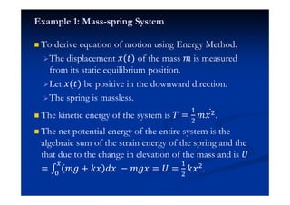
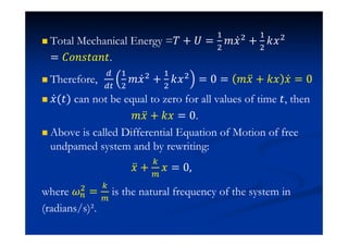
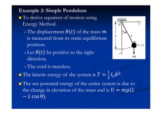
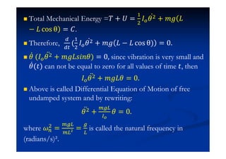
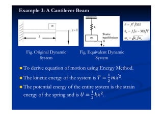
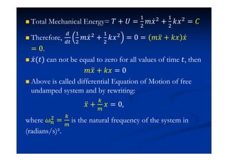
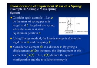
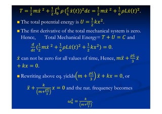
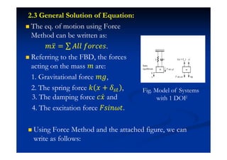

This document summarizes key concepts in vibration of single-degree-of-freedom (SDOF) systems. It discusses the generalized model of SDOF systems and provides examples. It then covers the differential equations of motion for SDOF systems using Newton's law and the energy method in the time domain. Specific examples are given for mass-spring, simple pendulum, and cantilever beam systems. Considerations for equivalent mass and stiffness of springs are also addressed.