This my presentation

1. Data Structures and Algorithms
Chapter One: Introduction to Data Structures
and Algorithms
Organized by Haymanot F.(MSc)

2. Contents
Introduction
Common Data Structures (Stacks, Queues, Lists, Trees,
Graphs, Tables)
ADT
Algorithm
Properties /Characteristics of an Algorithm
Measuring Complexity
Complexity of Algorithm
Asymptotic notation such as Big-oh notation and others
2

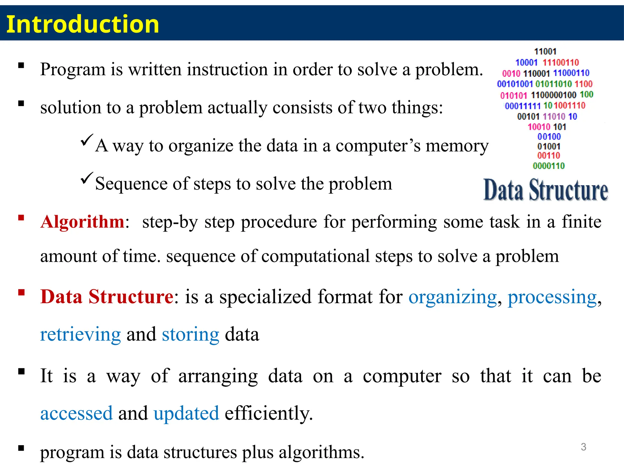
3.  Program is written instruction in order to solve a problem.
 solution to a problem actually consists of two things:
A way to organize the data in a computer’s memory
Sequence of steps to solve the problem
 Algorithm: step-by step procedure for performing some task in a finite
amount of time. sequence of computational steps to solve a problem
 Data Structure: is a specialized format for organizing, processing,
retrieving and storing data
 It is a way of arranging data on a computer so that it can be
accessed and updated efficiently.
 program is data structures plus algorithms. 3
Introduction

4. • For example, if you want to store data sequentially in the memory, then
you can go for the Array data structure.
• Note: Data structure and data types are slightly different.
• Data structure is the collection of data types arranged in a specific order.
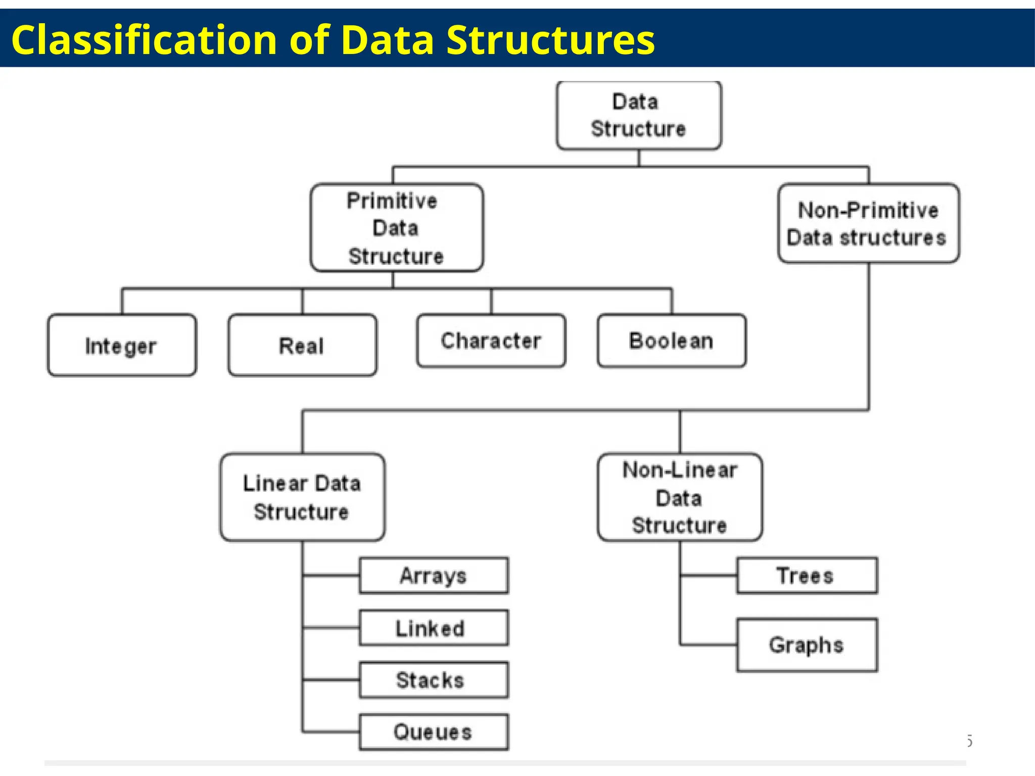
Types of Data Structure
• Linear data structure: elements are arranged in particular
order, they are easy to implement.
• However, when the complexity of the program increases, the
linear data structures might not be the best choice because of
operational complexities
• Non-linear data structure: elements arranged in a hierarchical manner
where one element will be connected to one or more elements
4
Introduction con…

5. 5
Classification of Data Structures

6. Cont..
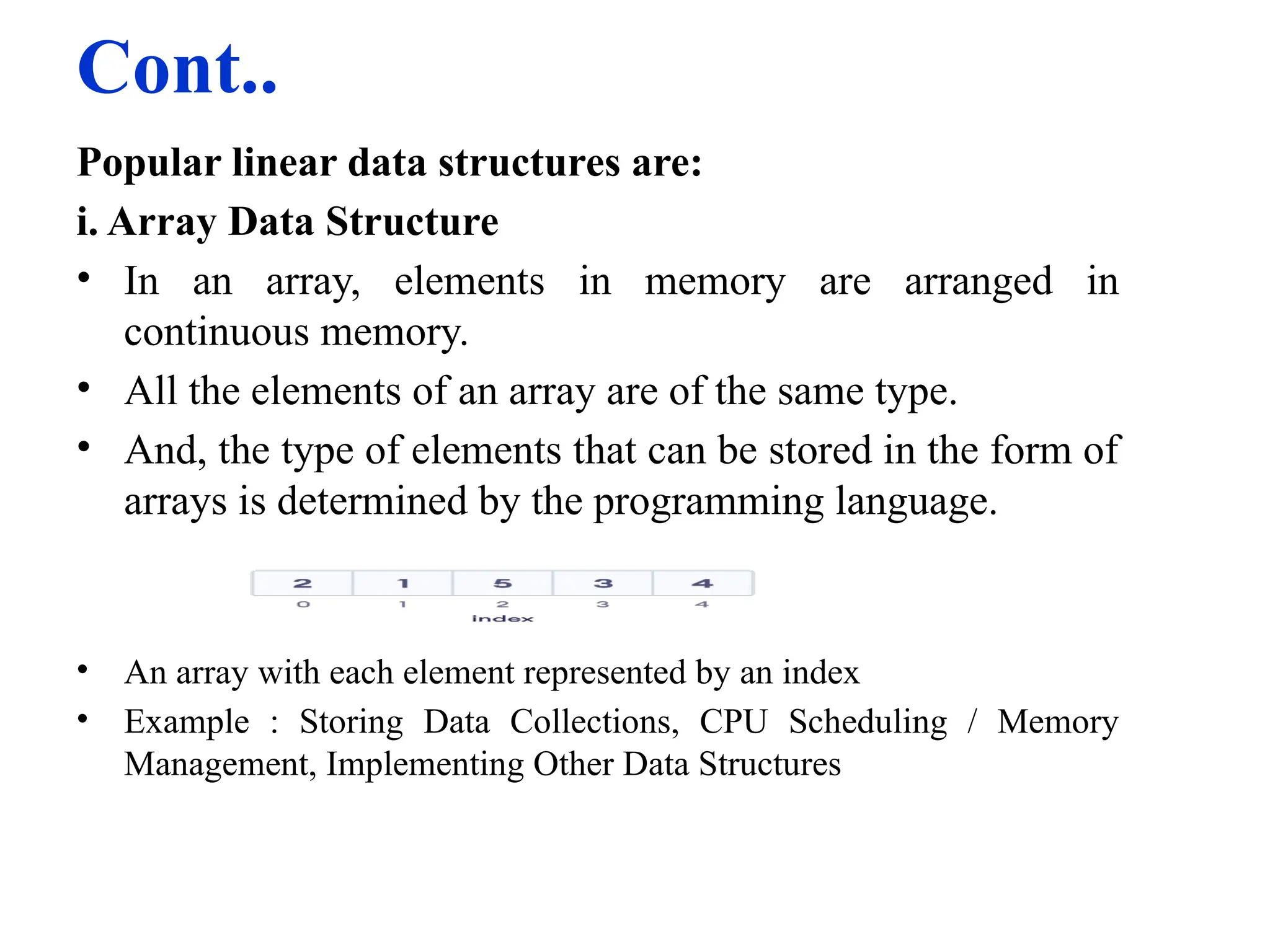
Popular linear data structures are:
i. Array Data Structure
• In an array, elements in memory are arranged in
continuous memory.
• All the elements of an array are of the same type.
• And, the type of elements that can be stored in the form of
arrays is determined by the programming language.
• An array with each element represented by an index
• Example : Storing Data Collections, CPU Scheduling / Memory
Management, Implementing Other Data Structures

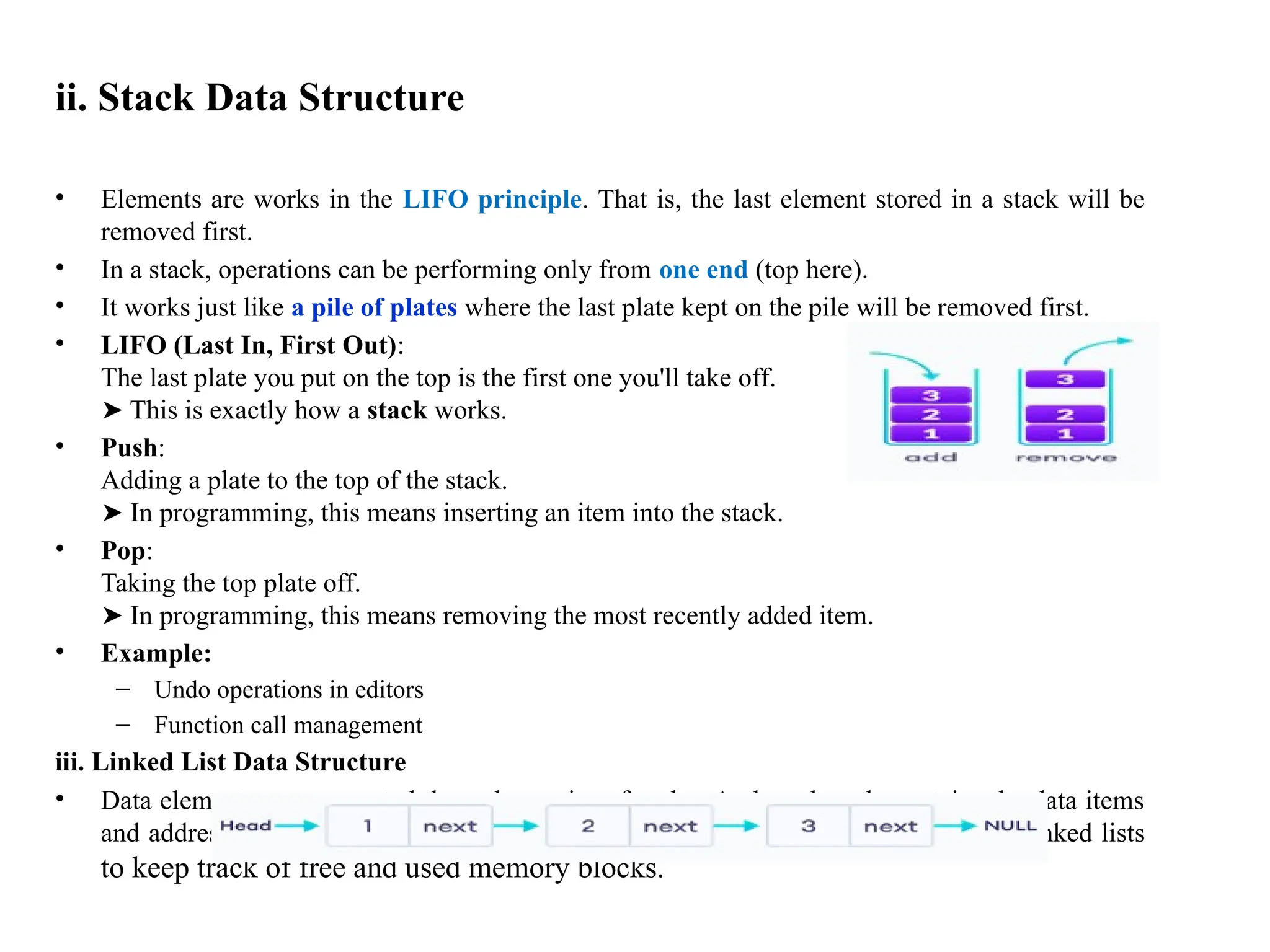
7. ii. Stack Data Structure
• Elements are works in the LIFO principle. That is, the last element stored in a stack will be
removed first.
• In a stack, operations can be performing only from one end (top here).
• It works just like a pile of plates where the last plate kept on the pile will be removed first.
• LIFO (Last In, First Out):
The last plate you put on the top is the first one you'll take off.
This is exactly how a
➤ stack works.
• Push:
Adding a plate to the top of the stack.
In programming, this means inserting an item into the stack.
➤
• Pop:
Taking the top plate off.
In programming, this means removing the most recently added item.
➤
• Example:
– Undo operations in editors
– Function call management
iii. Linked List Data Structure
• Data elements are connected through a series of nodes. And, each node contains the data items
and address to the next node. Example: Operating systems manage memory using linked lists
to keep track of free and used memory blocks.

8. 8
iv. Queue Data Structure
• Unlike stack, the queue data structure works in the FIFO principle where first
element stored in the queue will be removed first.
• First to join - first leave and last to join last to leave.
• It works just like a queue of people in the ticket counter where first person on
the queue will get the ticket first.
• Real life example:
• You join the end of the line → enqueue
• The person at the front gets the ticket and leaves → dequeue
• In a queue, addition and removal are performed from separate ends.
• Enqueue = Add data at the rear (end) of the queue
• Dequeue = Remove data from the front of the queue
Applications :
• Print queues
• Task scheduling in OS

9. Nonlinear data structures
• Unlike linear data structures, elements in non-linear data
structures are not in any sequence.
• Instead they are arranged in a hierarchical manner where one
element will be connected to one or more elements.
• Non-linear data structures are further divided into
A. Graph and
B. Tree based data structures

10. Cont..
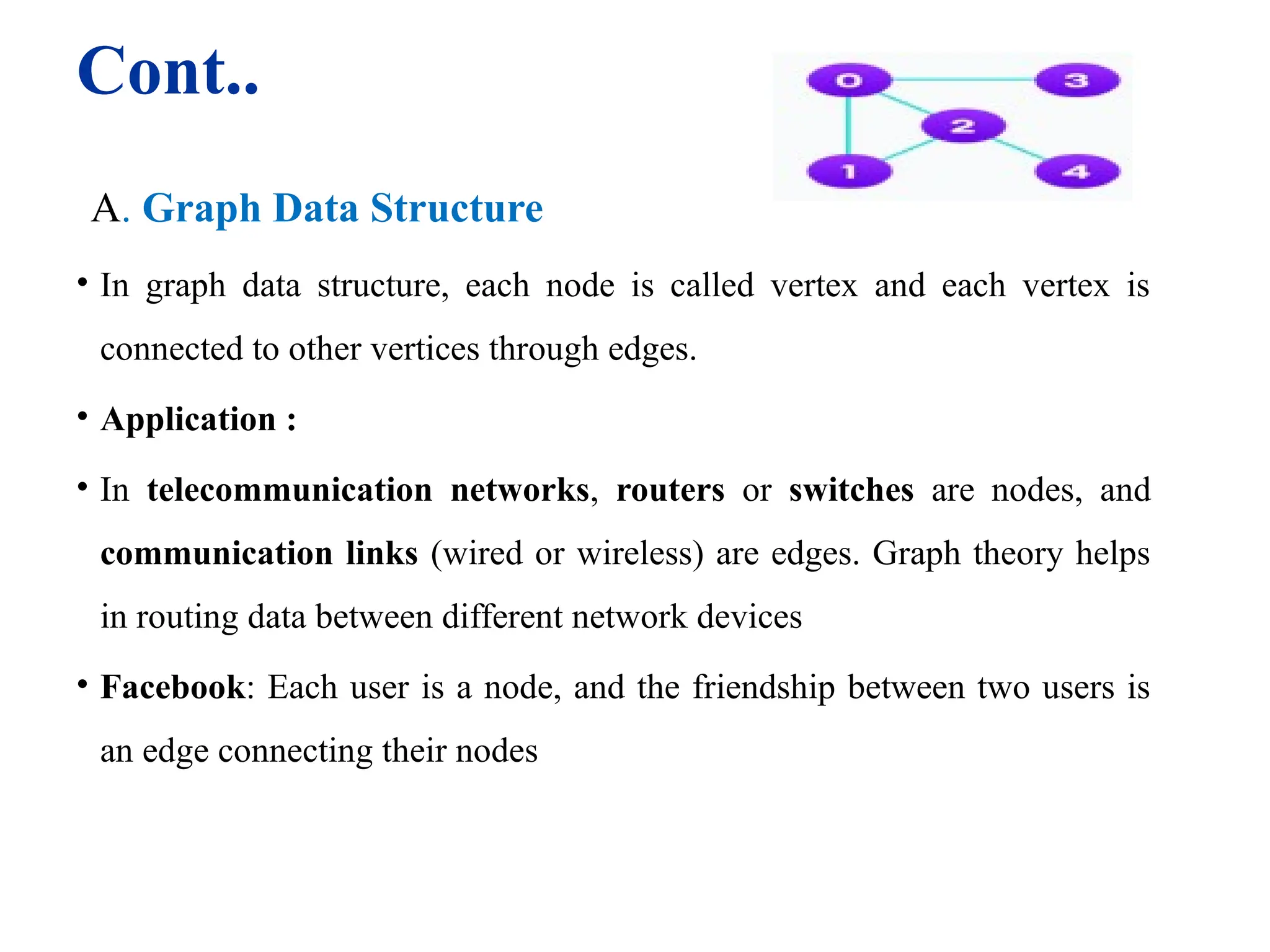
A. Graph Data Structure
• In graph data structure, each node is called vertex and each vertex is
connected to other vertices through edges.
• Application :
• In telecommunication networks, routers or switches are nodes, and
communication links (wired or wireless) are edges. Graph theory helps
in routing data between different network devices
• Facebook: Each user is a node, and the friendship between two users is
an edge connecting their nodes

11. Con…
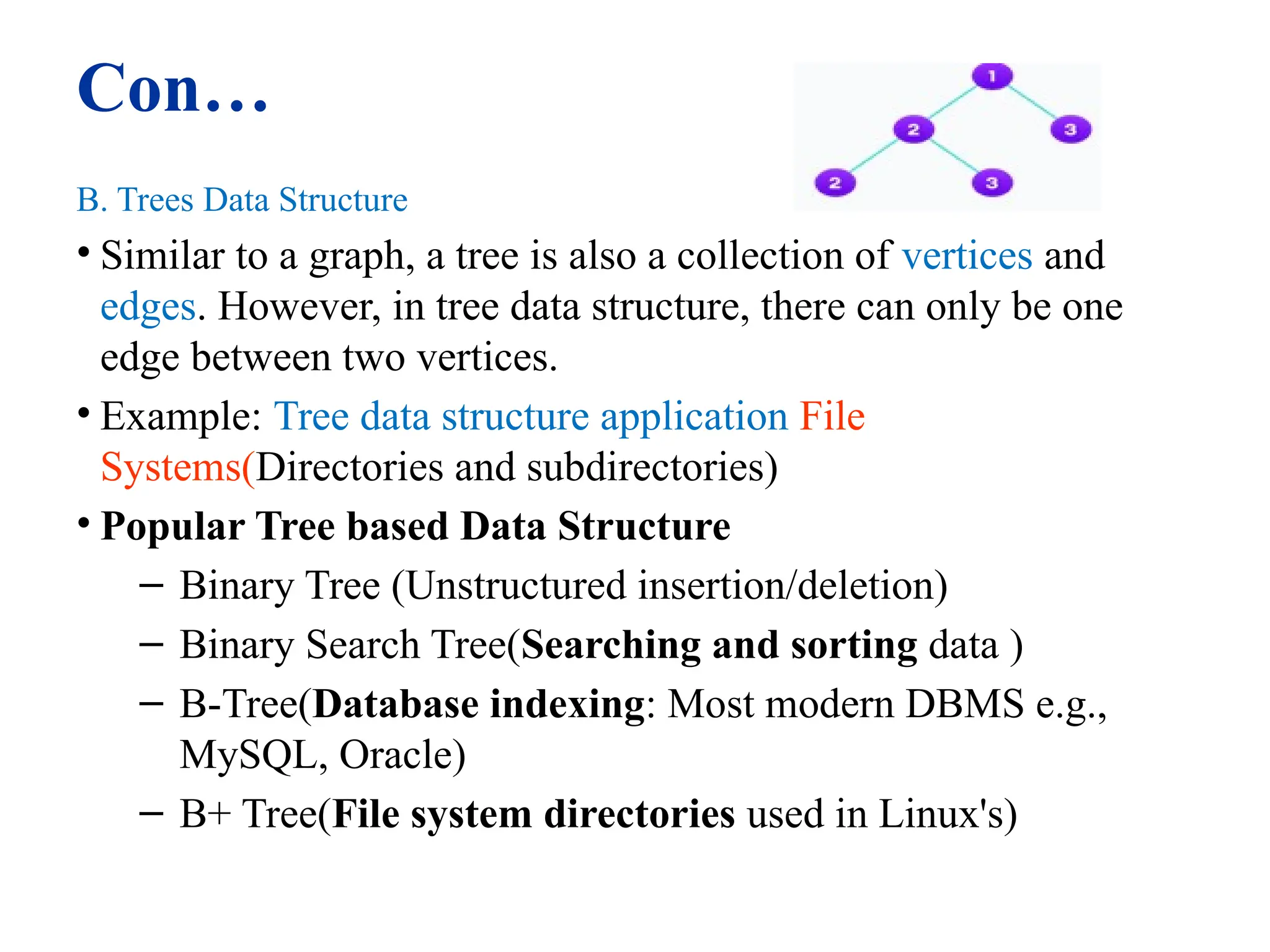
B. Trees Data Structure
• Similar to a graph, a tree is also a collection of vertices and
edges. However, in tree data structure, there can only be one
edge between two vertices.
• Example: Tree data structure application File
Systems(Directories and subdirectories)
• Popular Tree based Data Structure
– Binary Tree (Unstructured insertion/deletion)
– Binary Search Tree(Searching and sorting data )
– B-Tree(Database indexing: Most modern DBMS e.g.,
MySQL, Oracle)
– B+ Tree(File system directories used in Linux's)
11

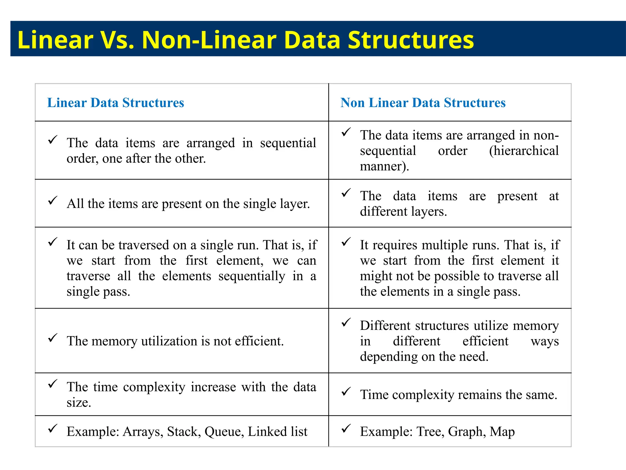
12. Linear Data Structures Non Linear Data Structures
 The data items are arranged in sequential
order, one after the other.
 The data items are arranged in non-
sequential order (hierarchical
manner).
 All the items are present on the single layer.
 The data items are present at
different layers.
 It can be traversed on a single run. That is, if
we start from the first element, we can
traverse all the elements sequentially in a
single pass.
 It requires multiple runs. That is, if
we start from the first element it
might not be possible to traverse all
the elements in a single pass.
 The memory utilization is not efficient.
 Different structures utilize memory
in different efficient ways
depending on the need.
 The time complexity increase with the data
size.
 Time complexity remains the same.
 Example: Arrays, Stack, Queue, Linked list  Example: Tree, Graph, Map
Linear Vs. Non-Linear Data Structures

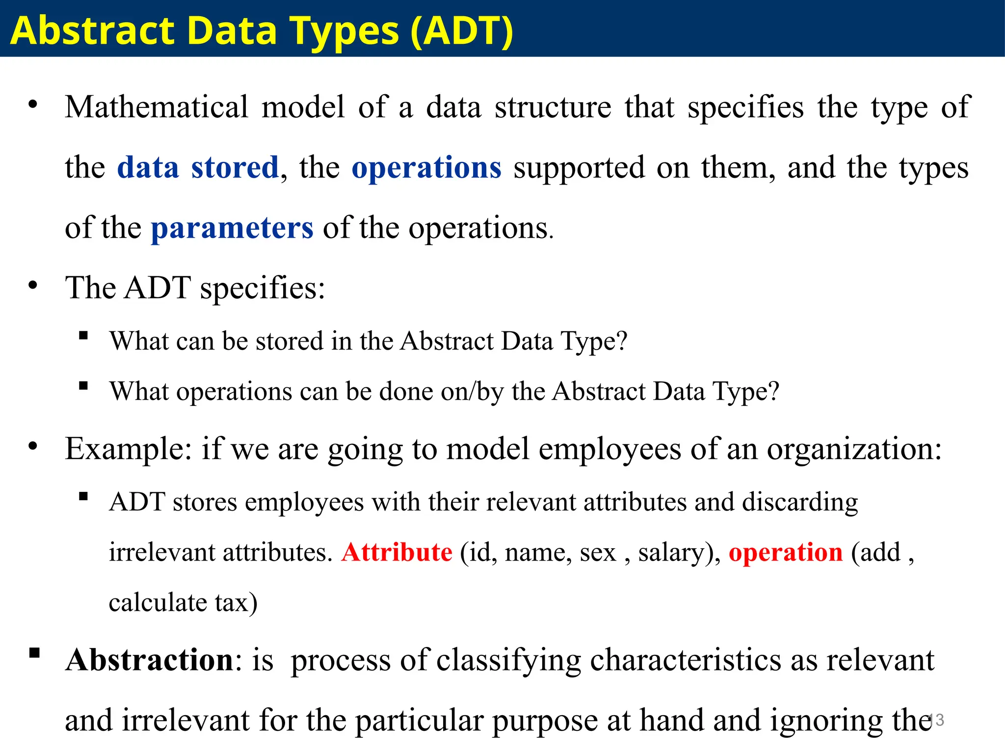
13. • Mathematical model of a data structure that specifies the type of
the data stored, the operations supported on them, and the types
of the parameters of the operations.
• The ADT specifies:
 What can be stored in the Abstract Data Type?
 What operations can be done on/by the Abstract Data Type?
• Example: if we are going to model employees of an organization:
 ADT stores employees with their relevant attributes and discarding
irrelevant attributes. Attribute (id, name, sex , salary), operation (add ,
calculate tax)
 Abstraction: is process of classifying characteristics as relevant
and irrelevant for the particular purpose at hand and ignoring the
13
Abstract Data Types (ADT)

14. • ADT is a theoretical model that defines the data structure behavior.
• Used to specify the data and the operation can be performed
• Deals about interface(abstract behavior) rather than implementation
• Data structure is implementation of ADT using memory and algorithm
• Data structure deals how data stored ,accessed and manipulate in
memory, how the operation performed on that data(via algorithm)
• Example list and stack are ADT support operations like insertion,
deletion, access for list and pop, push for stack
• List and stack ADT implement on data structure using array or linked
list
14
Abstract Data Types (ADT) con…

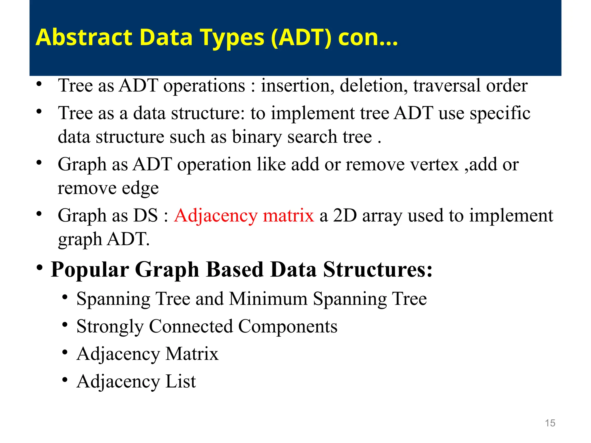
15. • Tree as ADT operations : insertion, deletion, traversal order
• Tree as a data structure: to implement tree ADT use specific
data structure such as binary search tree .
• Graph as ADT operation like add or remove vertex ,add or
remove edge
• Graph as DS : Adjacency matrix a 2D array used to implement
graph ADT.
• Popular Graph Based Data Structures:
• Spanning Tree and Minimum Spanning Tree
• Strongly Connected Components
• Adjacency Matrix
• Adjacency List
15
Abstract Data Types (ADT) con…

16. • It is well-defined procedure that takes some value or a set of values
as input and produces some value or a set of values as output.
• Algorithm are the dynamic part of a program’s world model.
• Data structures model the static part of the world, They are
unchanging while the world is changing.
• transforms data structures from one state to another state in two
ways:
– may change the value held by a data structure
– may change the data structure itself
• The quality of a data structure is related to its ability to
successfully model the characteristics of the world.
16
Algorithm

17. • The quality of an algorithm is related to its ability to
successfully simulate the changes in the world.
• correct data structures lead to simple and efficient
algorithms
• correct algorithms lead to accurate and efficient data
structures
• Algorithm example : binary search which search elements on
sorted array (Data structure) : binary search algorithm
implemented in array.
• Data structure is way of organize data
• Algorithm how to operate on data
17
Algorithm con…

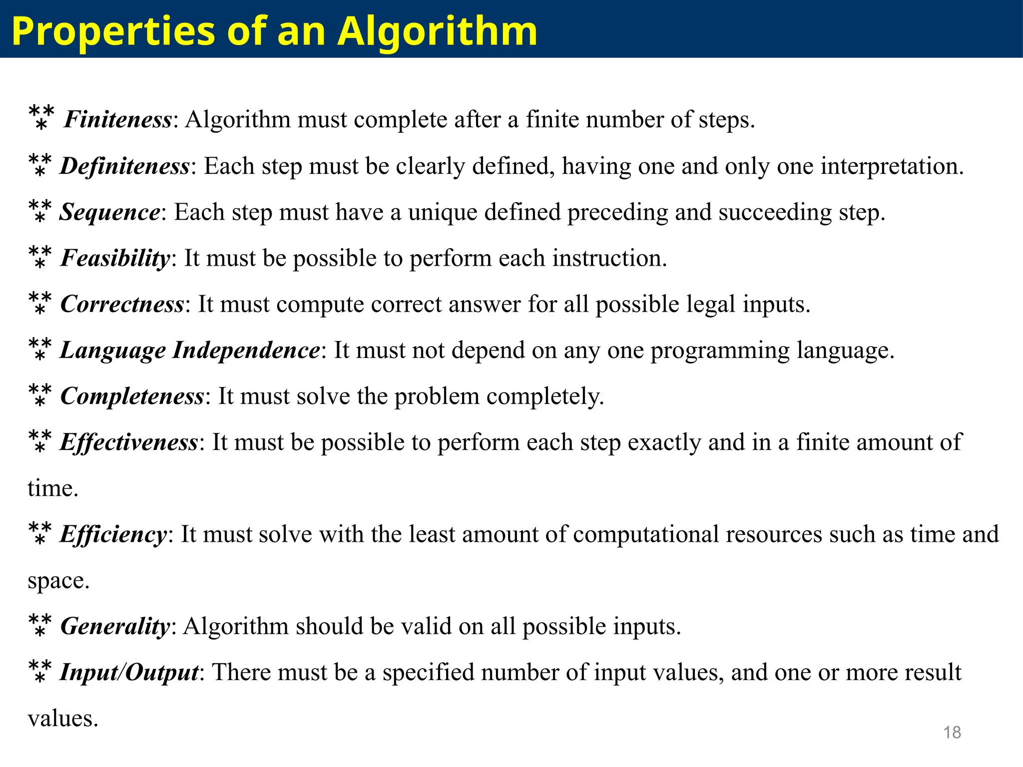
18.  Finiteness: Algorithm must complete after a finite number of steps.
 Definiteness: Each step must be clearly defined, having one and only one interpretation.
 Sequence: Each step must have a unique defined preceding and succeeding step.
 Feasibility: It must be possible to perform each instruction.
 Correctness: It must compute correct answer for all possible legal inputs.
 Language Independence: It must not depend on any one programming language.
 Completeness: It must solve the problem completely.
 Effectiveness: It must be possible to perform each step exactly and in a finite amount of
time.
 Efficiency: It must solve with the least amount of computational resources such as time and
space.
 Generality: Algorithm should be valid on all possible inputs.
 Input/Output: There must be a specified number of input values, and one or more result
values. 18
Properties of an Algorithm

19. Good Algorithms
• Run in less time
• Consume less memory
But computational resources (time complexity) is usually more important
Measuring Algorithms Efficiency
• The efficiency of an algorithm is a measure of the amount of
resources consumed in solving a problem of size n.
– The resource we are most interested in is time
– We can use the same techniques to analyze the consumption of other
resources, such as memory space.
• It would seem that the most obvious way to measure the efficiency of an
algorithm is to run it and measure how much processor time is needed.
19

20. Algorithm Analysis Concepts
• Algorithm analysis refers to the process of determining how
much computing time and storage that algorithms will
require.
• In other words, it’s a process of predicting the resource
requirement of algorithms in a given environment.
• In order to solve a problem, there are many possible algorithms.
One has to be able to choose the best algorithm for the problem
at hand using some scientific method.
• To classify some data structures and algorithms as good, we
need precise ways of analyzing them in terms of resource
20

21. Con…
• The main resources are:
– Running Time
– Memory Usage
• Running time is usually treated as the most important since
computational time is the most precious resource in most
problem domains.
• There are two approaches to measure the efficiency of
algorithms:
– Empirical
– Theoretical
21

22. • It works based on the total running time of the program. It uses actual
system clock time.
Example:
t1(Initial time before the program starts)
for(int i=0; i<=10; i++)
cout<<i;
t2 (final time after the execution of the program is finished)
Running time taken by the above algorithm (TotalTime) = t2-t1;
• It is difficult to determine efficiency of algorithms using this approach,
because clock-time can vary based on many factors. For example:
a) Processor speed of the computer
b) Current processor load
c) Specific data for a particular run of the program (Input Size and
Input Properties)
d) Operating System
• Multitasking Vs.Single tasking
• Internal structure
1. Empirical Algorithm Analysis
22

23. • Determining the quantity of resources required using mathematical
concept.
• Analyze an algorithm according to the number of basic operations (time
units) required, rather than according to an absolute amount of time
involved.
• We use theoretical approach to determine the efficiency of algorithm
because:
– The number of operation will not vary under different conditions.
– It helps us to have a meaningful measure that permits comparison of
algorithms independent of operating platform.
– It helps to determine the complexity of algorithm(the amount of
2. Theoretical Algorithm Analysis
23

24. • Complexity Analysis determines the amount of time and space
resources required to solve a problem, with respect to input size
• It is a theoretical way to estimate how efficient an algorithm is,
especially as the input grows large
• and it stays independent of hardware and software differences
• It is the process of evaluating how the resources needed by an
algorithm grow with the size of the input
• Instead of measuring actual execution time, it uses asymptotic
notation like: O(n) linear, O(n²) quadratic
• This abstract view helps compare algorithms theoretically, no matter
where or how they're implemented.
Complexity Analysis
24

25. • Goal: a meaningful measure that permits
• comparison of algorithms independent of operating platform.
• choosing or designing the right algorithm for the problem.
• Two important ways to characterize the effectiveness of an
algorithm
– Time Complexity: Determine the approximate number of
operations required to solve a problem of size n.
– Space Complexity: Determine the approximate memory
required to solve a problem of size n.
– The running time of an algorithm is a function of the input
size.
Complexity Analysis
25

26. Complexity analysis involves two distinct phases:
1. Algorithm Analysis: Analysis of the algorithm or data structure to
produce a function T(n) that describes the algorithm in terms of
the operations performed in order to measure the complexity of
the algorithm.
2. Order of Magnitude Analysis: Analysis of the function T (n) to
determine the general complexity category to which it belongs
(constant time, linear time, logarithmic time, quadratic time,
exponential time or other).
Complexity Analysis
26

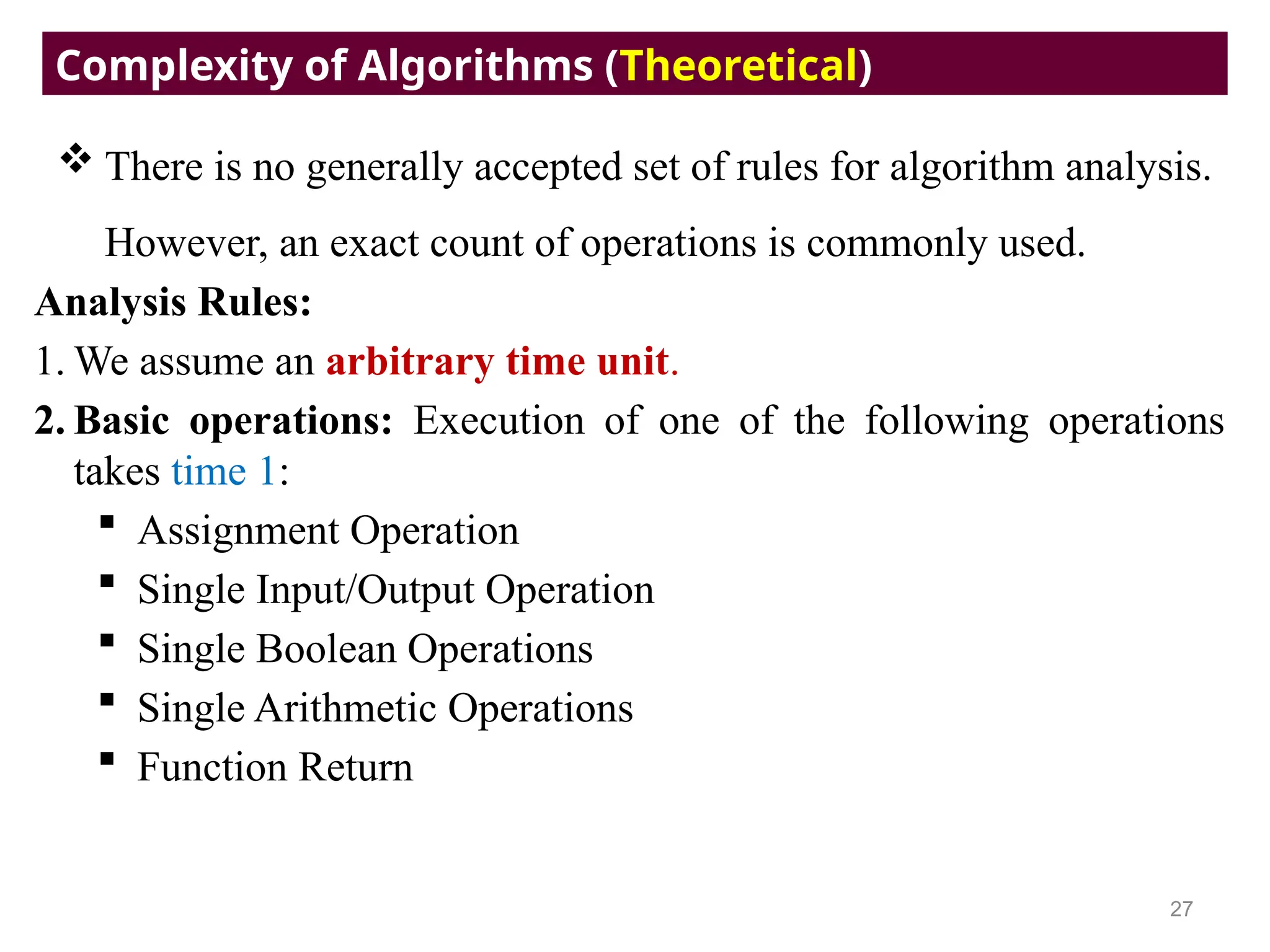
27.  There is no generally accepted set of rules for algorithm analysis.
However, an exact count of operations is commonly used.
Analysis Rules:
1. We assume an arbitrary time unit.
2. Basic operations: Execution of one of the following operations
takes time 1:
 Assignment Operation
 Single Input/Output Operation
 Single Boolean Operations
 Single Arithmetic Operations
 Function Return
Complexity of Algorithms (Theoretical)
27

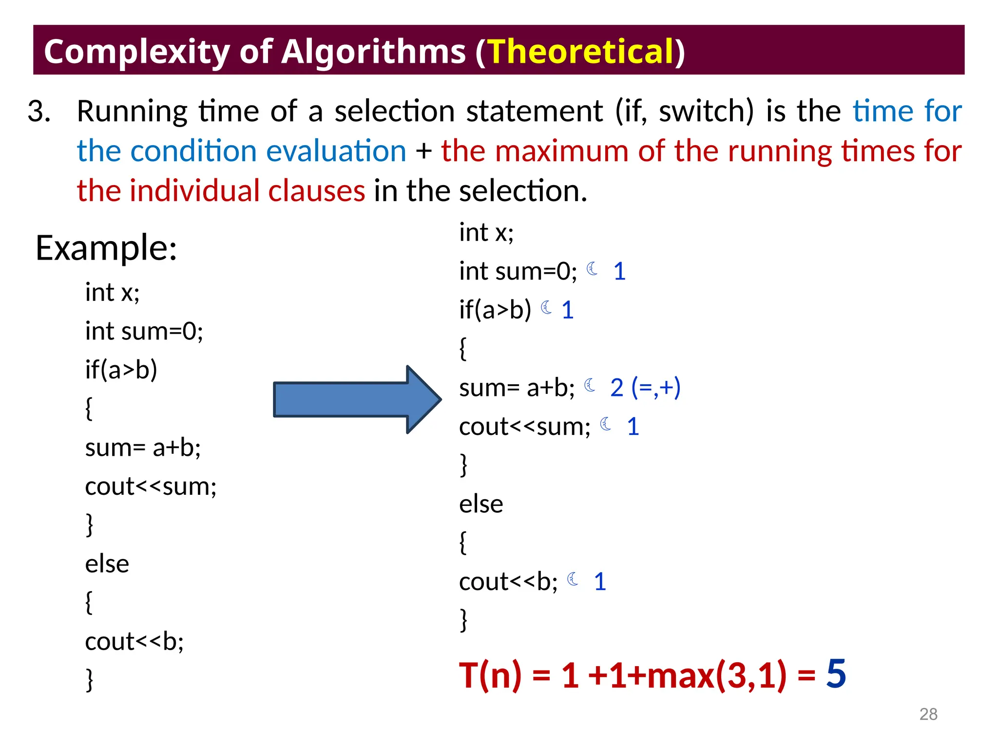
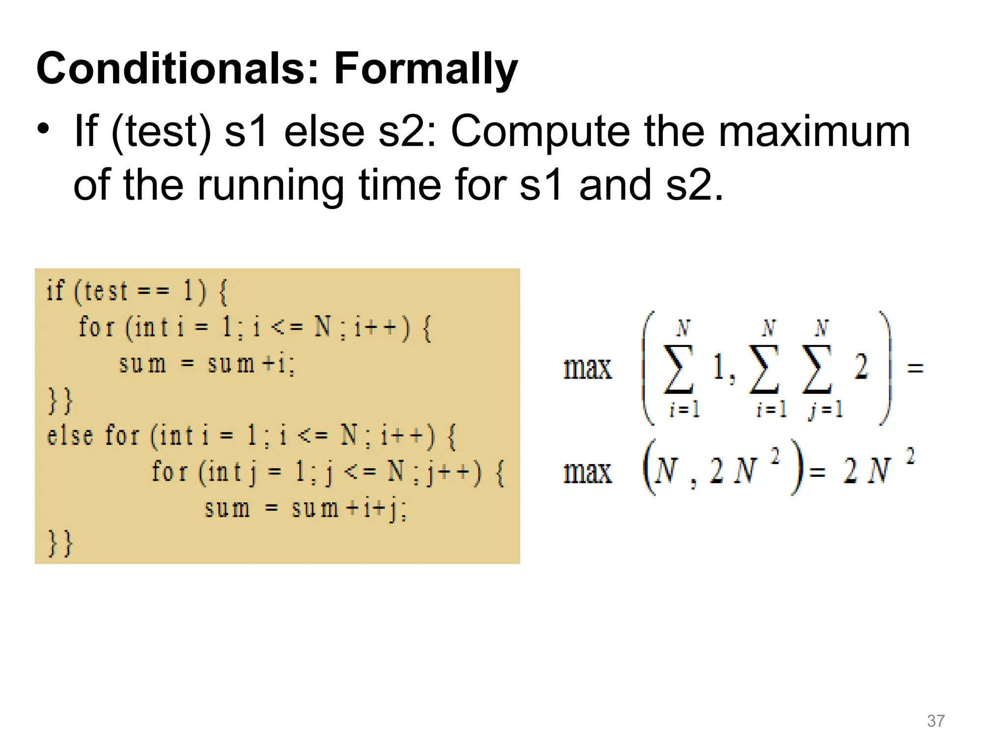
28. 3. Running time of a selection statement (if, switch) is the time for
the condition evaluation + the maximum of the running times for
the individual clauses in the selection.
Complexity of Algorithms (Theoretical)
28
Example:
int x;
int sum=0;
if(a>b)
{
sum= a+b;
cout<<sum;
}
else
{
cout<<b;
}
int x;
int sum=0; 1
if(a>b)1
{
sum= a+b; 2 (=,+)
cout<<sum; 1
}
else
{
cout<<b; 1
}
T(n) = 1 +1+max(3,1) = 5

29. 29
4. Loop statements
 The running time for the statements inside the loop*number of
iterations + time for setup ( 1 ) + time for checking ( number of
iteration + 1 ) + time for update ( number of iteration ) .
 The total running time of statements inside a group of nested
loops is the running time of the statements*the product of the
sizes of all the loops.
 For nested loops , analyze inside out . Always assume that the
loop executes the maximum number of iterations possible .

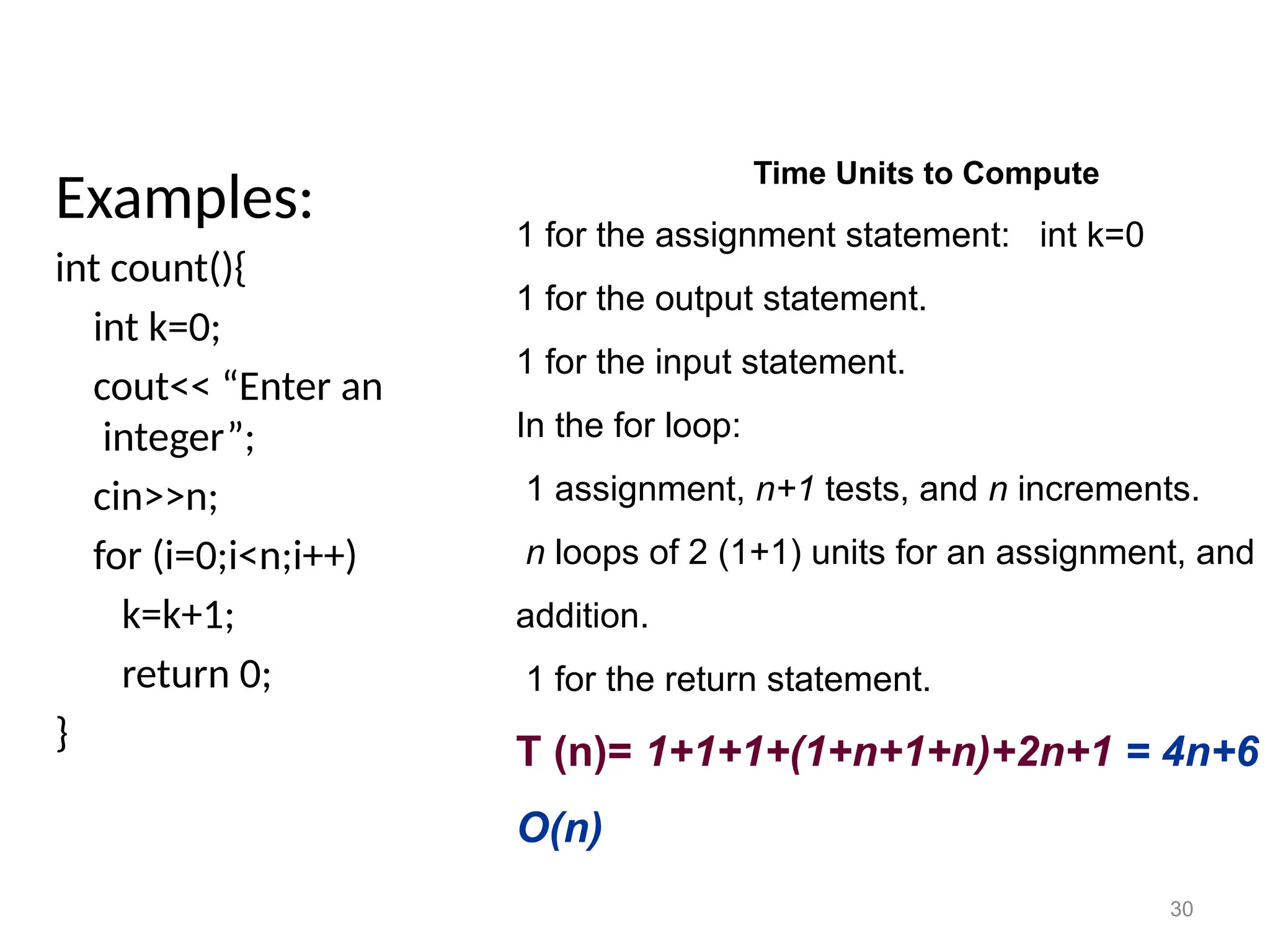
30. Examples:
int count(){
int k=0;
cout<< “Enter an
integer”;
cin>>n;
for (i=0;i<n;i++)
k=k+1;
return 0;
}
Time Units to Compute
1 for the assignment statement: int k=0
1 for the output statement.
1 for the input statement.
In the for loop:
1 assignment, n+1 tests, and n increments.
n loops of 2 (1+1) units for an assignment, and
addition.
1 for the return statement.
T (n)= 1+1+1+(1+n+1+n)+2n+1 = 4n+6
O(n)
30

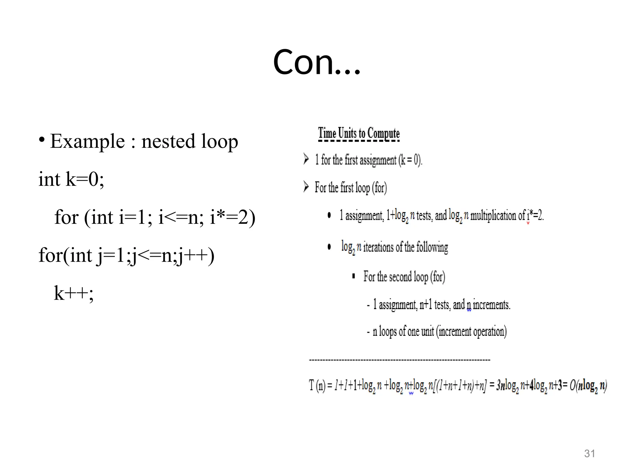
31. Con…
• Example : nested loop
int k=0;
for (int i=1; i<=n; i*=2)
for(int j=1;j<=n;j++)
k++;
31

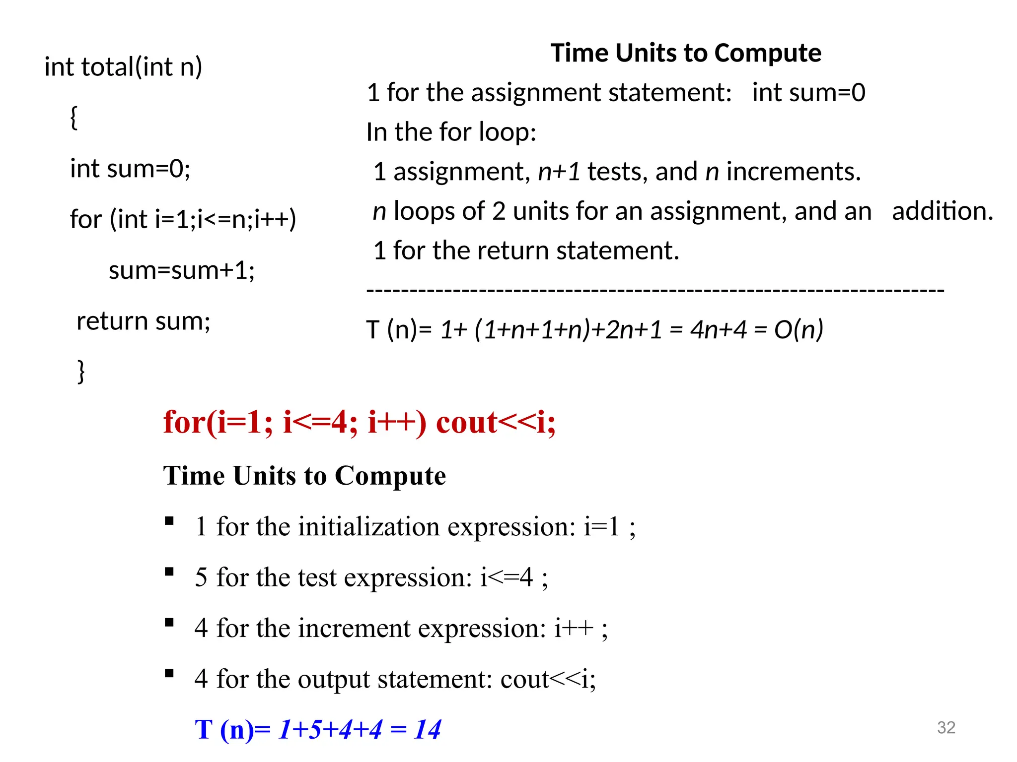
32. int total(int n)
{
int sum=0;
for (int i=1;i<=n;i++)
sum=sum+1;
return sum;
}
Time Units to Compute
1 for the assignment statement: int sum=0
In the for loop:
1 assignment, n+1 tests, and n increments.
n loops of 2 units for an assignment, and an addition.
1 for the return statement.
-------------------------------------------------------------------
T (n)= 1+ (1+n+1+n)+2n+1 = 4n+4 = O(n)
32
for(i=1; i<=4; i++) cout<<i;
Time Units to Compute
 1 for the initialization expression: i=1 ;
 5 for the test expression: i<=4 ;
 4 for the increment expression: i++ ;
 4 for the output statement: cout<<i;
T (n)= 1+5+4+4 = 14

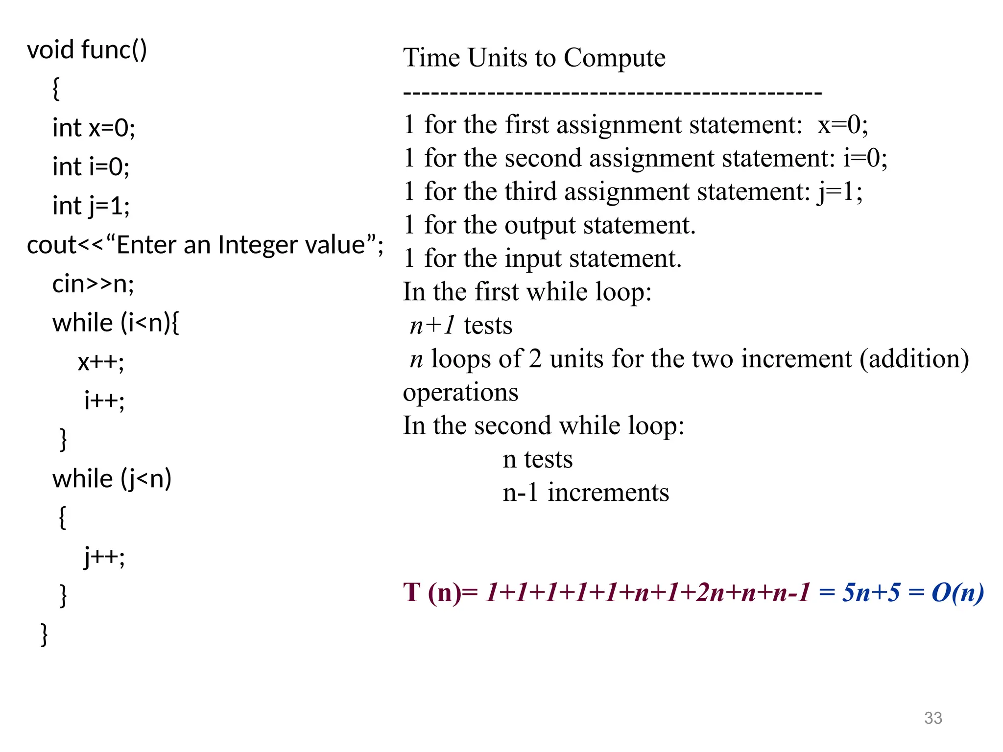
33. void func()
{
int x=0;
int i=0;
int j=1;
cout<<“Enter an Integer value”;
cin>>n;
while (i<n){
x++;
i++;
}
while (j<n)
{
j++;
}
}
Time Units to Compute
---------------------------------------------
1 for the first assignment statement: x=0;
1 for the second assignment statement: i=0;
1 for the third assignment statement: j=1;
1 for the output statement.
1 for the input statement.
In the first while loop:
n+1 tests
n loops of 2 units for the two increment (addition)
operations
In the second while loop:
n tests
n-1 increments
T (n)= 1+1+1+1+1+n+1+2n+n+n-1 = 5n+5 = O(n)
33

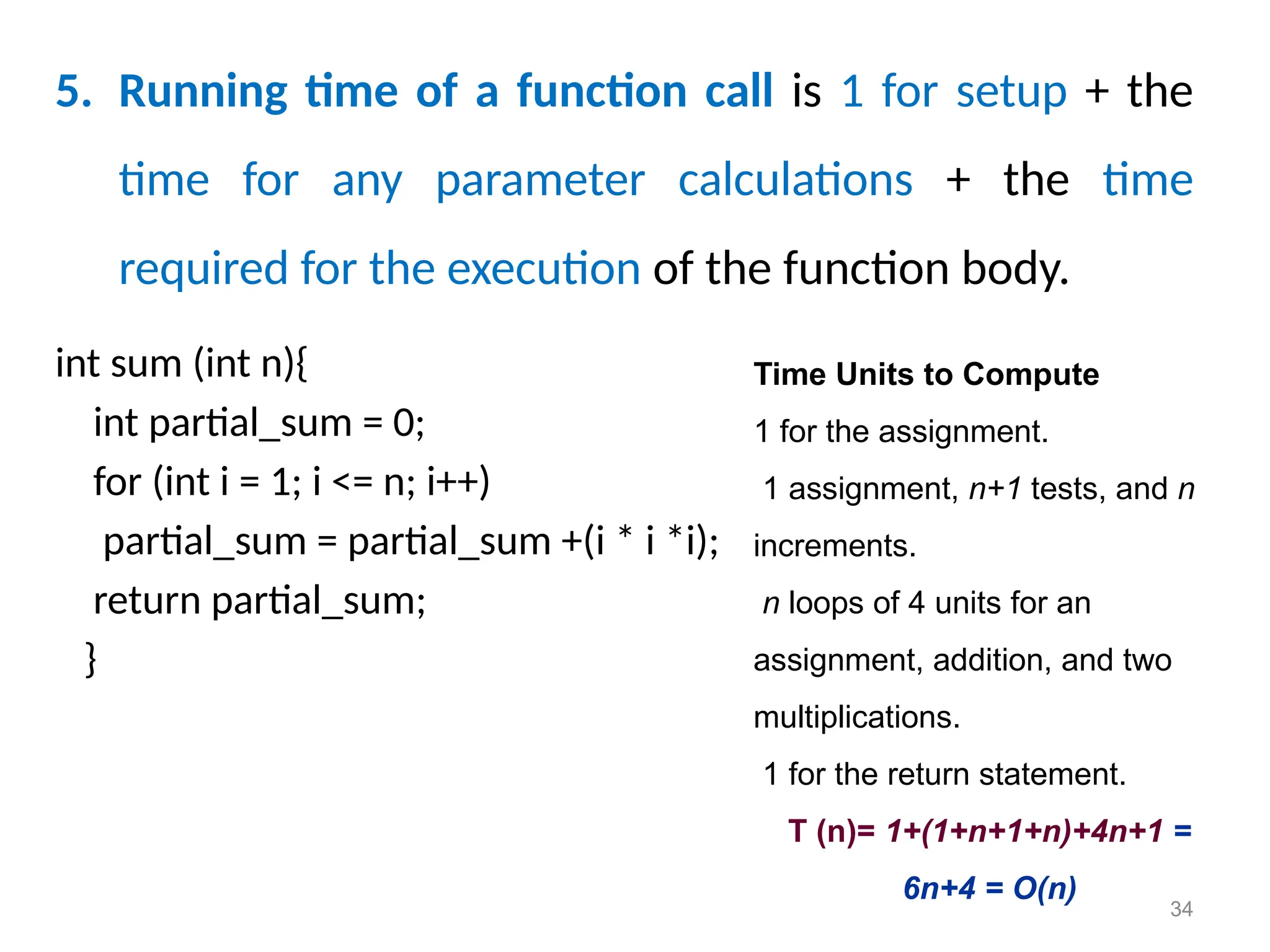
34. 5. Running time of a function call is 1 for setup + the
time for any parameter calculations + the time
required for the execution of the function body.
34
Time Units to Compute
1 for the assignment.
1 assignment, n+1 tests, and n
increments.
n loops of 4 units for an
assignment, addition, and two
multiplications.
1 for the return statement.
T (n)= 1+(1+n+1+n)+4n+1 =
6n+4 = O(n)
int sum (int n){
int partial_sum = 0;
for (int i = 1; i <= n; i++)
partial_sum = partial_sum +(i * i *i);
return partial_sum;
}

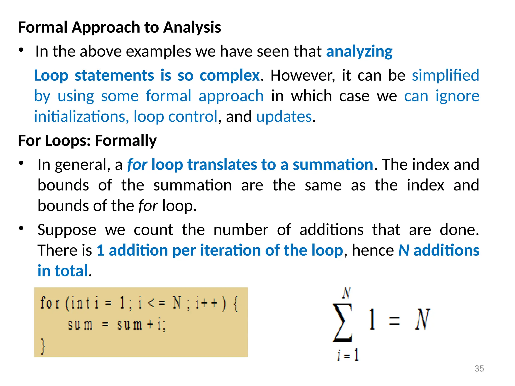
35. Formal Approach to Analysis
• In the above examples we have seen that analyzing
Loop statements is so complex. However, it can be simplified
by using some formal approach in which case we can ignore
initializations, loop control, and updates.
For Loops: Formally
• In general, a for loop translates to a summation. The index and
bounds of the summation are the same as the index and
bounds of the for loop.
• Suppose we count the number of additions that are done.
There is 1 addition per iteration of the loop, hence N additions
in total.
35

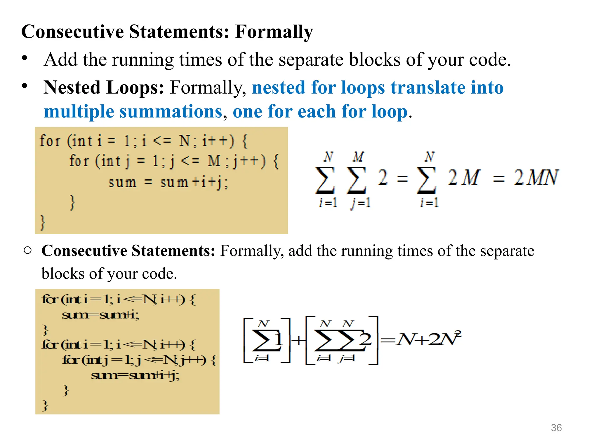
36. Consecutive Statements: Formally
• Add the running times of the separate blocks of your code.
• Nested Loops: Formally, nested for loops translate into
multiple summations, one for each for loop.
o Consecutive Statements: Formally, add the running times of the separate
blocks of your code.
36

37. Conditionals: Formally
• If (test) s1 else s2: Compute the maximum
of the running time for s1 and s2.
37

38. Con…
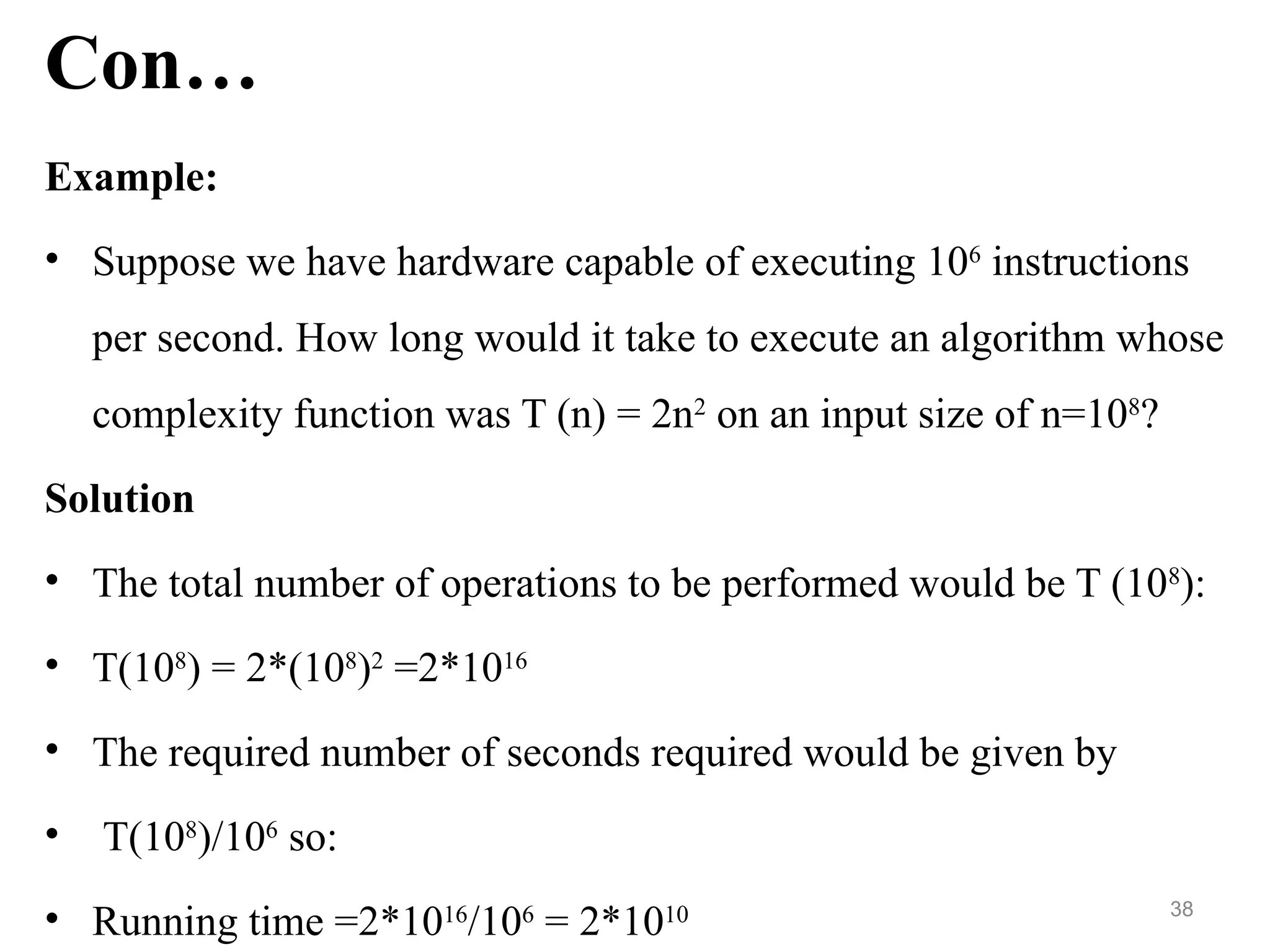
Example:
• Suppose we have hardware capable of executing 106
instructions
per second. How long would it take to execute an algorithm whose
complexity function was T (n) = 2n2
on an input size of n=108
?
Solution
• The total number of operations to be performed would be T (108
):
• T(108
) = 2*(108
)2
=2*1016
• The required number of seconds required would be given by
• T(108
)/106
so:
• Running time =2*1016
/106
= 2*1010 38

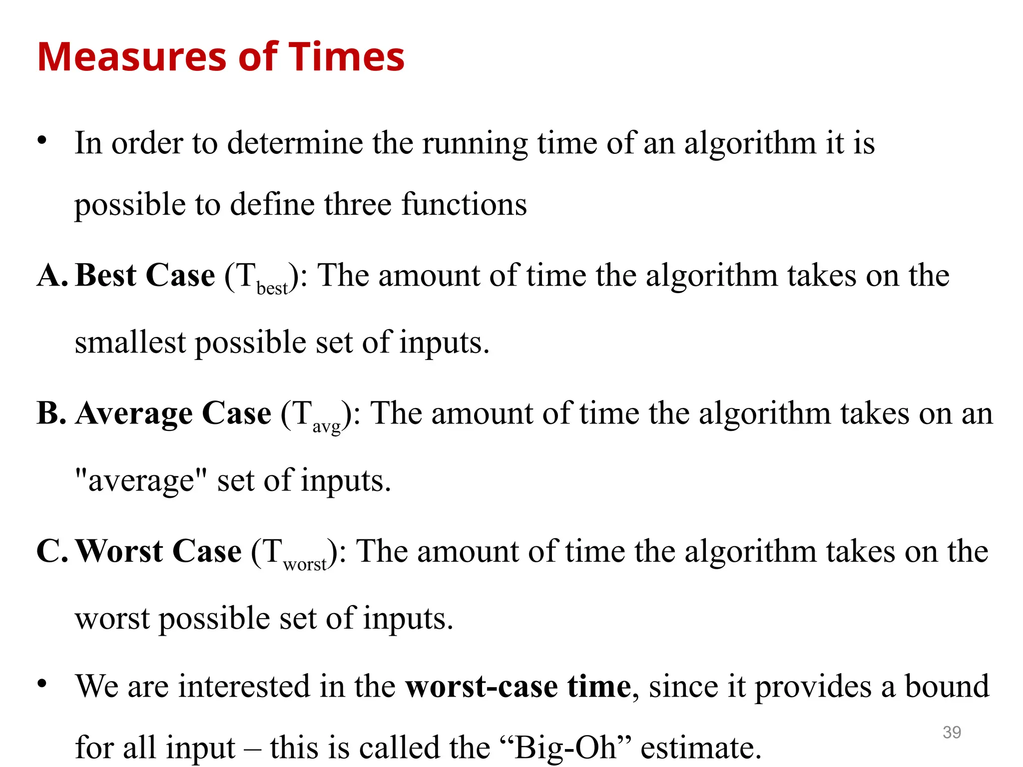
39. Measures of Times
• In order to determine the running time of an algorithm it is
possible to define three functions
A. Best Case (Tbest): The amount of time the algorithm takes on the
smallest possible set of inputs.
B. Average Case (Tavg): The amount of time the algorithm takes on an
"average" set of inputs.
C. Worst Case (Tworst): The amount of time the algorithm takes on the
worst possible set of inputs.
• We are interested in the worst-case time, since it provides a bound
for all input – this is called the “Big-Oh” estimate.
39

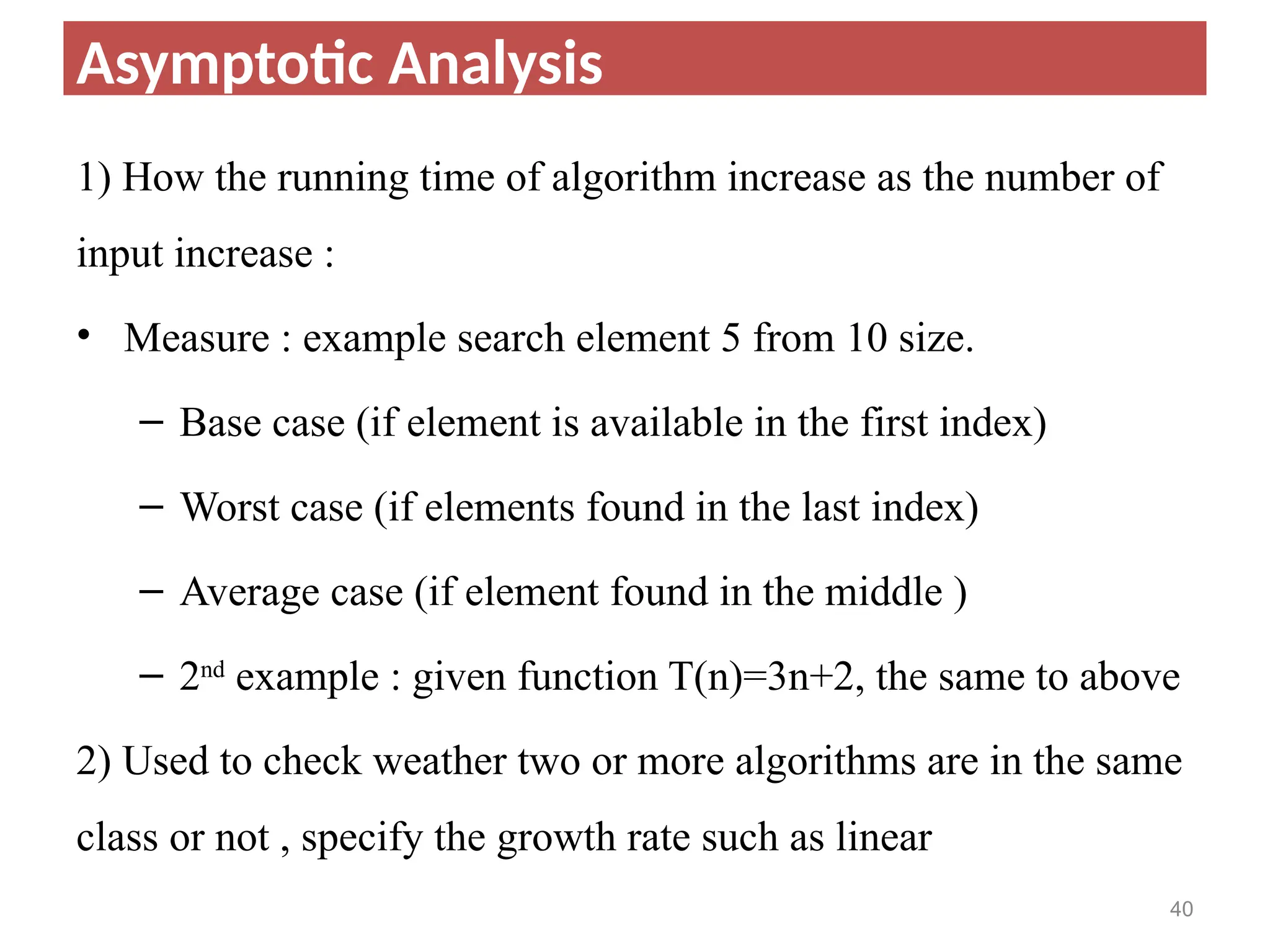
40. 1) How the running time of algorithm increase as the number of
input increase :
• Measure : example search element 5 from 10 size.
– Base case (if element is available in the first index)
– Worst case (if elements found in the last index)
– Average case (if element found in the middle )
– 2nd
example : given function T(n)=3n+2, the same to above
2) Used to check weather two or more algorithms are in the same
class or not , specify the growth rate such as linear
40
Asymptotic Analysis

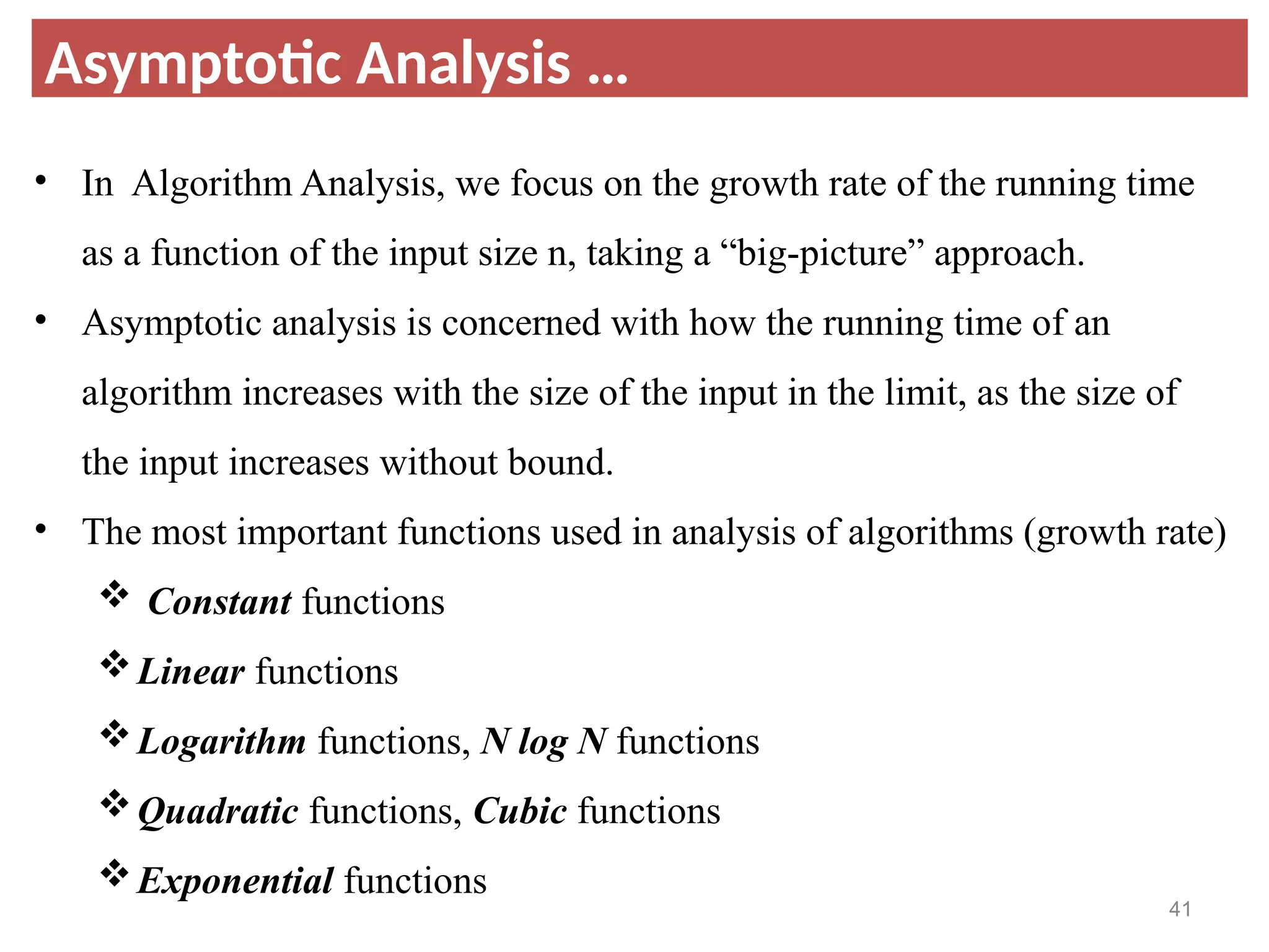
41. Asymptotic Analysis …
• In Algorithm Analysis, we focus on the growth rate of the running time
as a function of the input size n, taking a “big-picture” approach.
• Asymptotic analysis is concerned with how the running time of an
algorithm increases with the size of the input in the limit, as the size of
the input increases without bound.
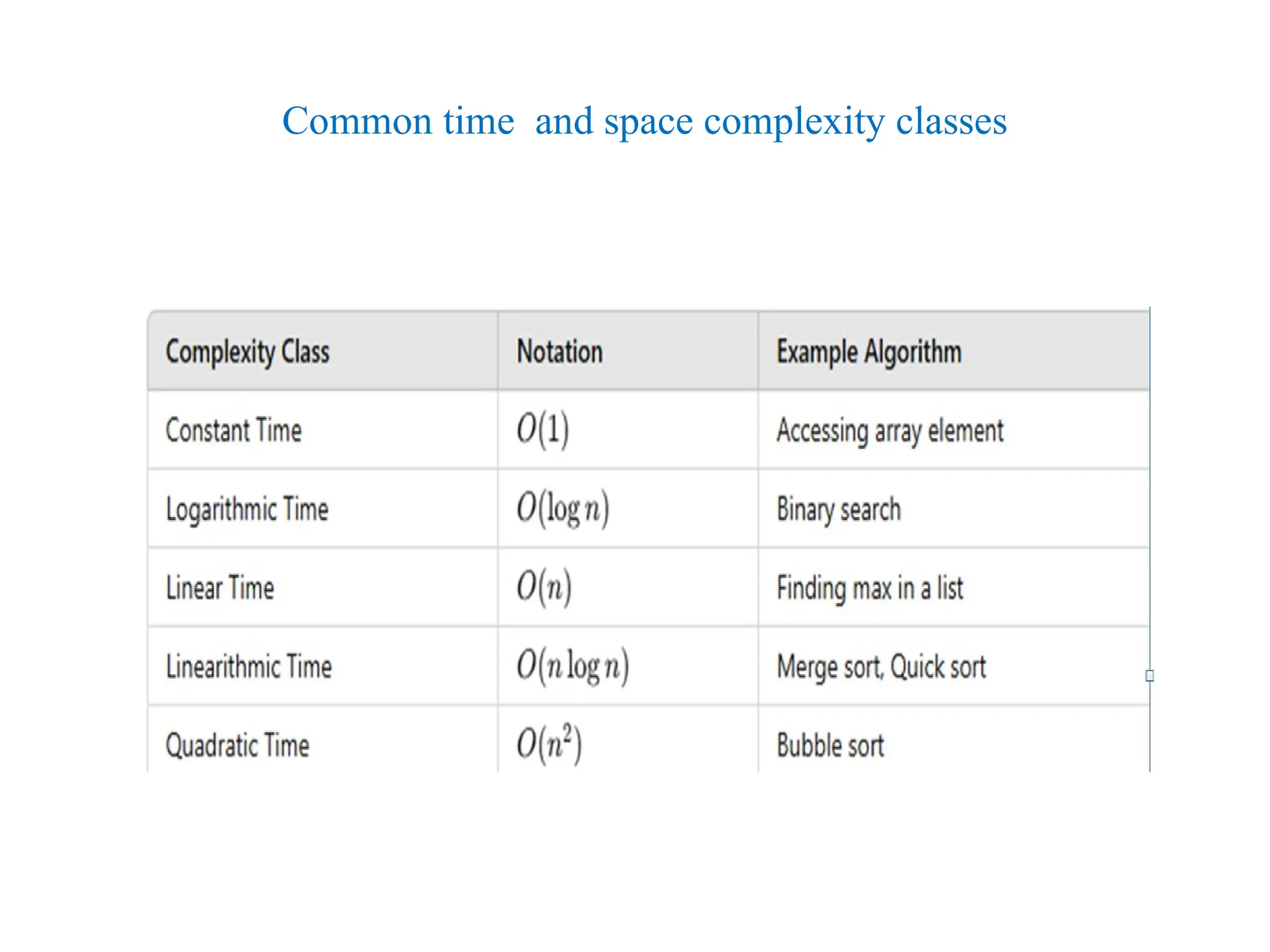
• The most important functions used in analysis of algorithms (growth rate)
 Constant functions
Linear functions
Logarithm functions, N log N functions
Quadratic functions, Cubic functions
Exponential functions
41

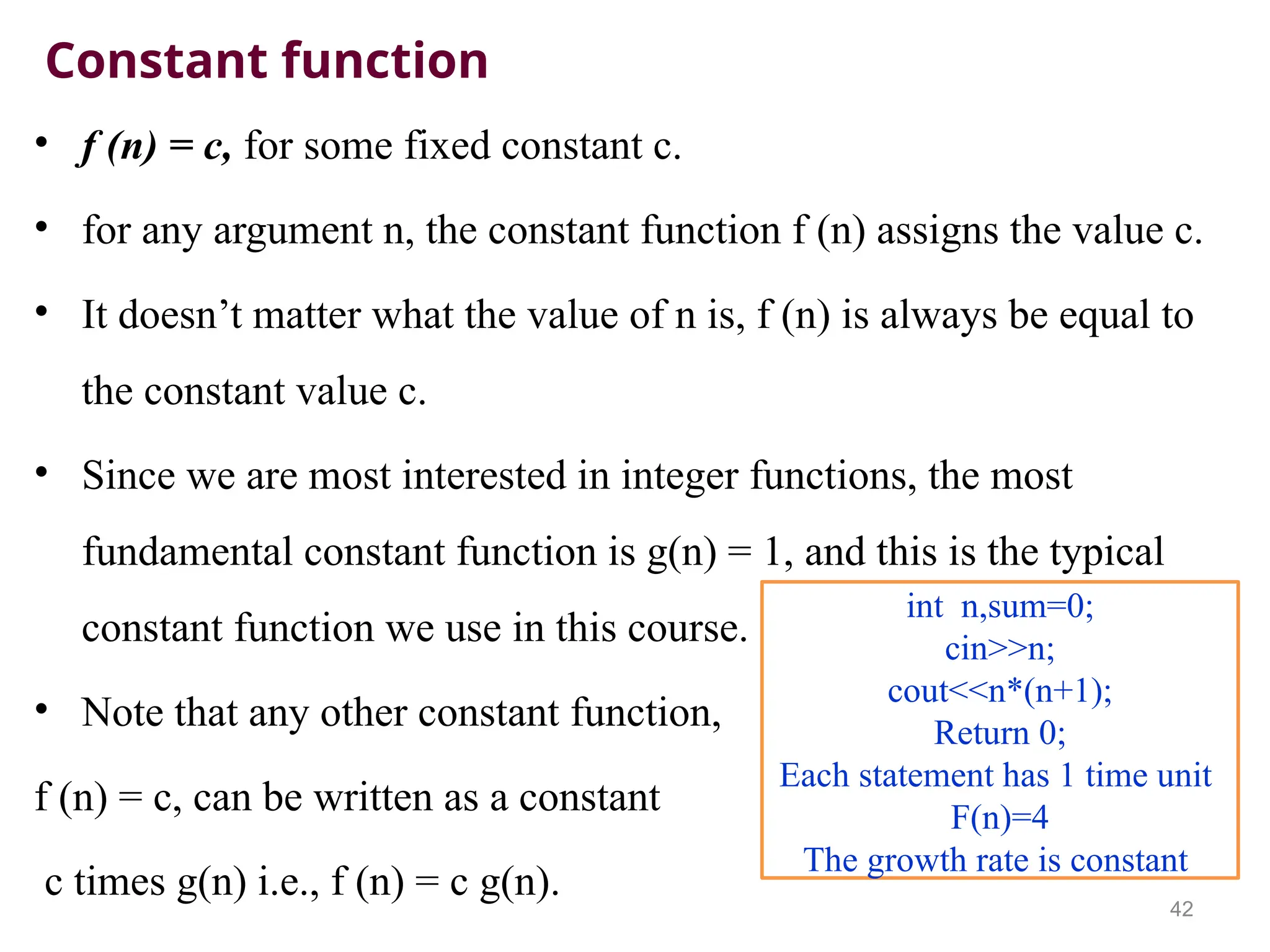
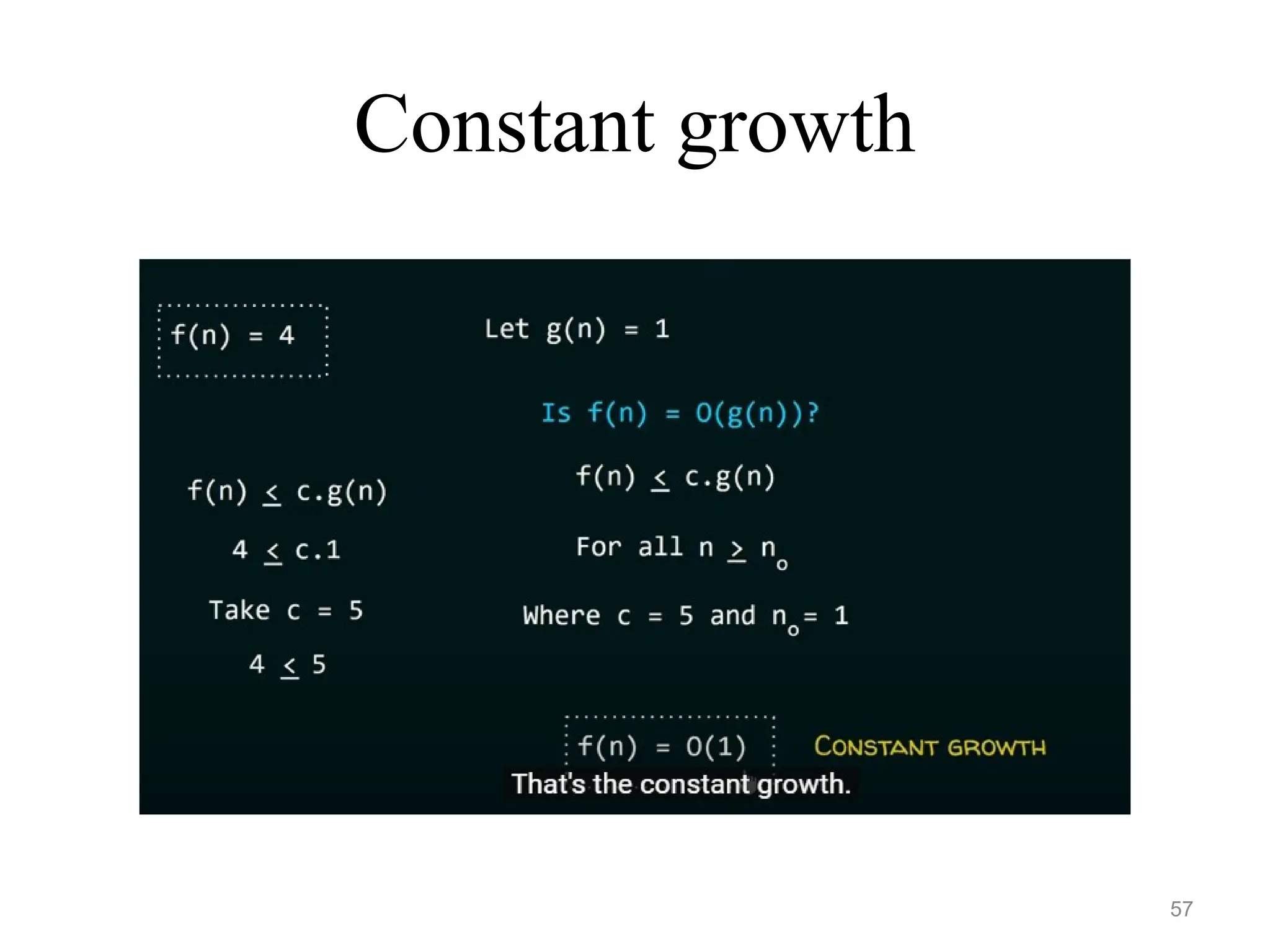
42. Constant function
• f (n) = c, for some fixed constant c.
• for any argument n, the constant function f (n) assigns the value c.
• It doesn’t matter what the value of n is, f (n) is always be equal to
the constant value c.
• Since we are most interested in integer functions, the most
fundamental constant function is g(n) = 1, and this is the typical
constant function we use in this course.
• Note that any other constant function,
f (n) = c, can be written as a constant
c times g(n) i.e., f (n) = c g(n).
42
int n,sum=0;
cin>>n;
cout<<n*(n+1);
Return 0;
Each statement has 1 time unit
F(n)=4
The growth rate is constant

43. Linear function
• f (n) = n.
• given an input value n, the linear function f assigns the value n
itself.
• This function arises in algorithm analysis any time we have to do a
single basic operation for each of n elements.
• Example: comparing a number x to each element of an array of size
n requires n comparisons.
43
bool findElement(int arr[], int n, int key){
for (int i = 0; i < n; i++) {
if (arr[i] == key) {
return true; }
return false;}
the growth rate is linear

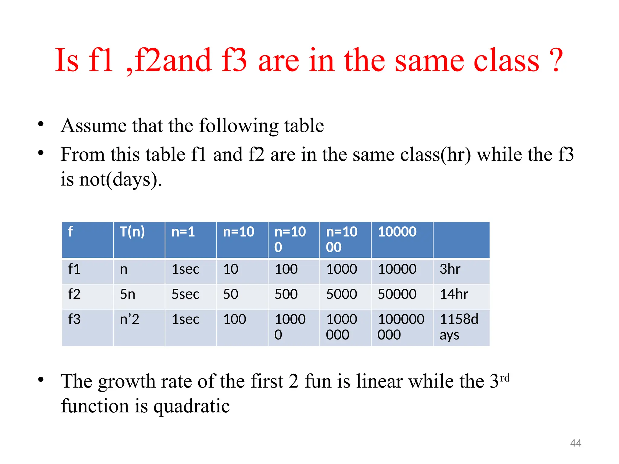
44. Is f1 ,f2and f3 are in the same class ?
44
f T(n) n=1 n=10 n=10
0
n=10
00
10000
f1 n 1sec 10 100 1000 10000 3hr
f2 5n 5sec 50 500 5000 50000 14hr
f3 n’2 1sec 100 1000
0
1000
000
100000
000
1158d
ays
• Assume that the following table
• From this table f1 and f2 are in the same class(hr) while the f3
is not(days).
• The growth rate of the first 2 fun is linear while the 3rd
function is quadratic

45. Logarithm function
• f (n) = logbn for some constant b > 1.
• defined as x = logbn if and only if bx
= n. By
definition, logb1 = 0.
for (int i=1;i<=n)
{ i=i*2;}
• n=2^k-1
• k-1=log2n
• K=log2n+1
• f(n)=o(log2n)
45
Iteration 1 i=1 2^0
Iteration 2 i=2 2^1
Iteration 3 i=4 2^2
Iteration k i=n 2^k-1
for (int i=1;i<=32)
{ cout<<“hello”;
i=i*2;}
k= log2 32+1= 6

46. Quadratic function
• f (n) = n2
• given an input value n, the function f assigns the product of n with itself (in other
words, “n squared”).
• main reason: there are many algorithms that have nested loops
– inner loop performs a linear number of operations
– outer loop is performed a linear number of times.
Thus, the algorithm performs n*n = n2
operations.
46
void bubbleSort(int arr[], int n){
for (int i = 0; i < n - 1; i++) {
for (int j = 0; j < n - i - 1; j++) {
if (arr[j] > arr[j + 1]) {
swap(&arr[j], &arr[j + 1]);
}} }}

47. Cubic function
• f (n) = n3
• assigns to an input value n the product of n with itself three times.
• appears less frequently in the context of algorithm analysis than the
constant, linear, and quadratic functions.
47
void multiply(int mat1[][N], int mat2[][N], int
res[][N]){
for (int i = 0; i < N; i++) {
for (int j = 0; j < N; j++) {
res[i][j] = 0;
for (int k = 0; k < N; k++)
res[i][j] += mat1[i][k] * mat2[k][j];
}}}

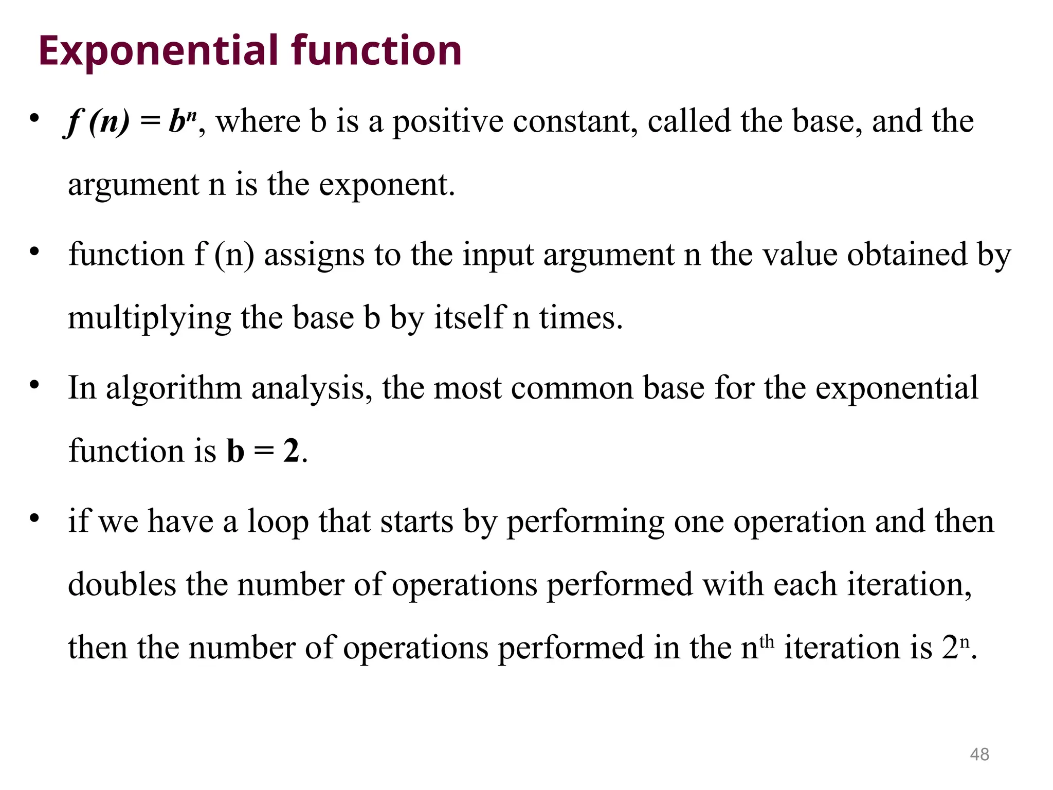
48. Exponential function
• f (n) = bn
, where b is a positive constant, called the base, and the
argument n is the exponent.
• function f (n) assigns to the input argument n the value obtained by
multiplying the base b by itself n times.
• In algorithm analysis, the most common base for the exponential
function is b = 2.
• if we have a loop that starts by performing one operation and then
doubles the number of operations performed with each iteration,
then the number of operations performed in the nth
iteration is 2n
.
48

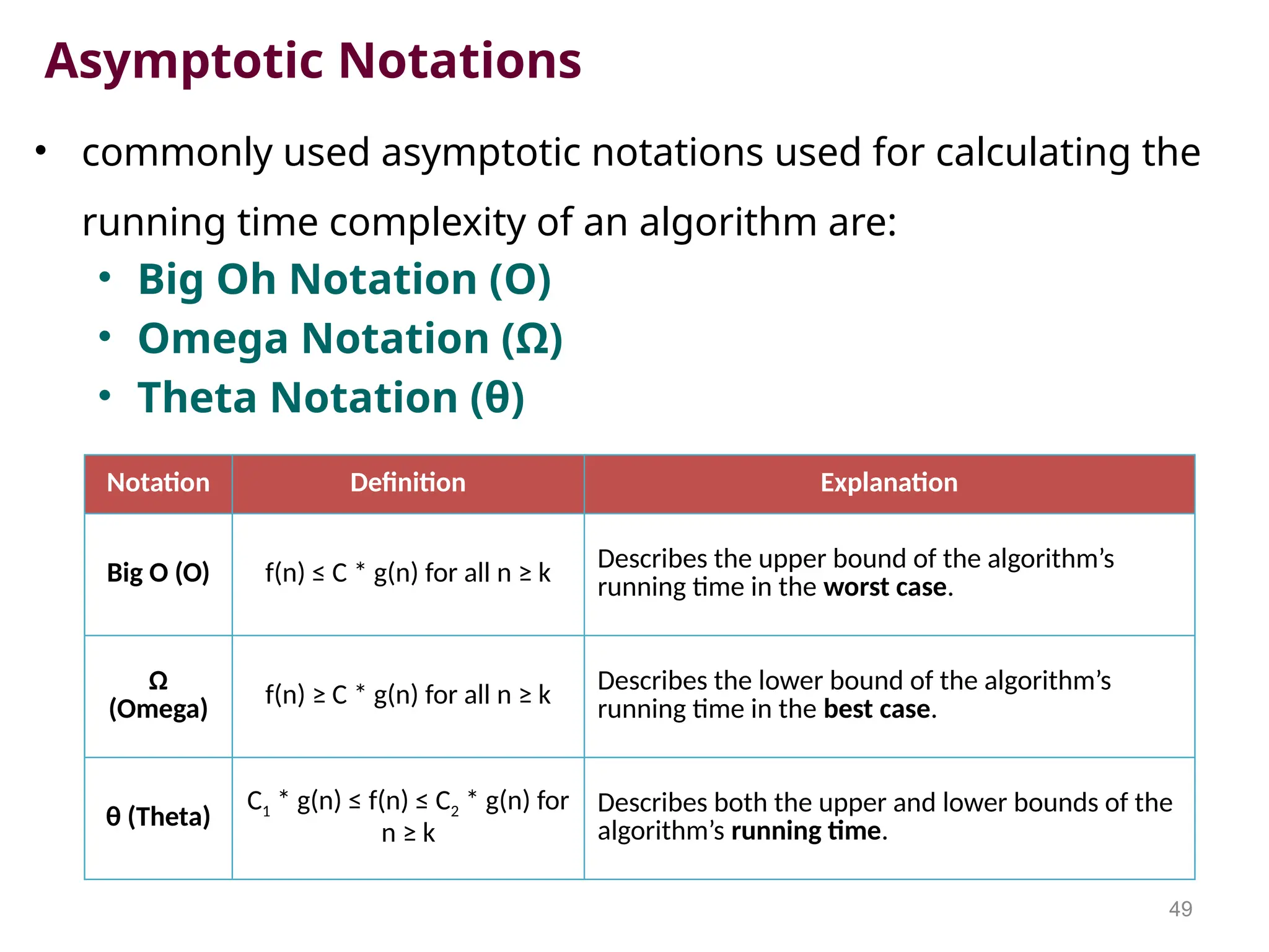
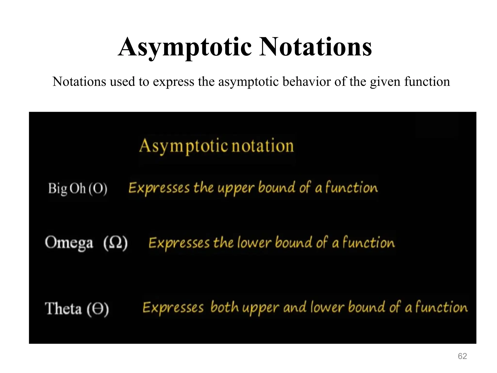
49. Asymptotic Notations
• commonly used asymptotic notations used for calculating the
running time complexity of an algorithm are:
• Big Oh Notation (O)
• Omega Notation (Ω)
• Theta Notation (θ)
49
Notation Definition Explanation
Big O (O) f(n) ≤ C * g(n) for all n ≥ k
Describes the upper bound of the algorithm’s
running time in the worst case.
Ω
(Omega)
f(n) ≥ C * g(n) for all n ≥ k
Describes the lower bound of the algorithm’s
running time in the best case.
θ (Theta)
C1 * g(n) ≤ f(n) ≤ C2 * g(n) for
n ≥ k
Describes both the upper and lower bounds of the
algorithm’s running time.

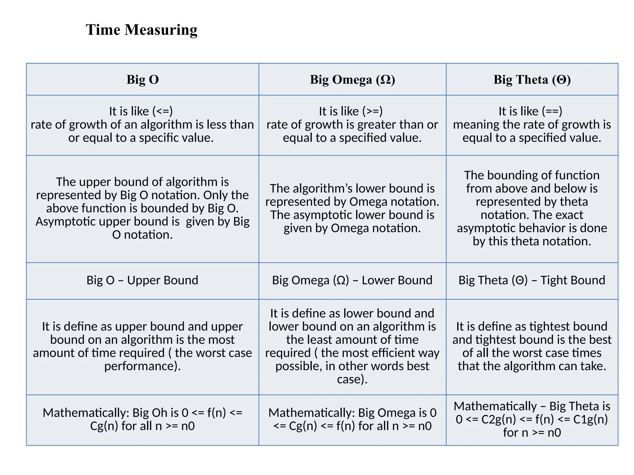
50. Big O Big Omega (Ω) Big Theta (Θ)
It is like (<=)
rate of growth of an algorithm is less than
or equal to a specific value.
It is like (>=)
rate of growth is greater than or
equal to a specified value.
It is like (==)
meaning the rate of growth is
equal to a specified value.
The upper bound of algorithm is
represented by Big O notation. Only the
above function is bounded by Big O.
Asymptotic upper bound is given by Big
O notation.
The algorithm’s lower bound is
represented by Omega notation.
The asymptotic lower bound is
given by Omega notation.
The bounding of function
from above and below is
represented by theta
notation. The exact
asymptotic behavior is done
by this theta notation.
Big O – Upper Bound Big Omega (Ω) – Lower Bound Big Theta (Θ) – Tight Bound
It is define as upper bound and upper
bound on an algorithm is the most
amount of time required ( the worst case
performance).
It is define as lower bound and
lower bound on an algorithm is
the least amount of time
required ( the most efficient way
possible, in other words best
case).
It is define as tightest bound
and tightest bound is the best
of all the worst case times
that the algorithm can take.
Mathematically: Big Oh is 0 <= f(n) <=
Cg(n) for all n >= n0
Mathematically: Big Omega is 0
<= Cg(n) <= f(n) for all n >= n0
Mathematically – Big Theta is
0 <= C2g(n) <= f(n) <= C1g(n)
for n >= n0
50
Time Measuring

51. Big-Oh Notation
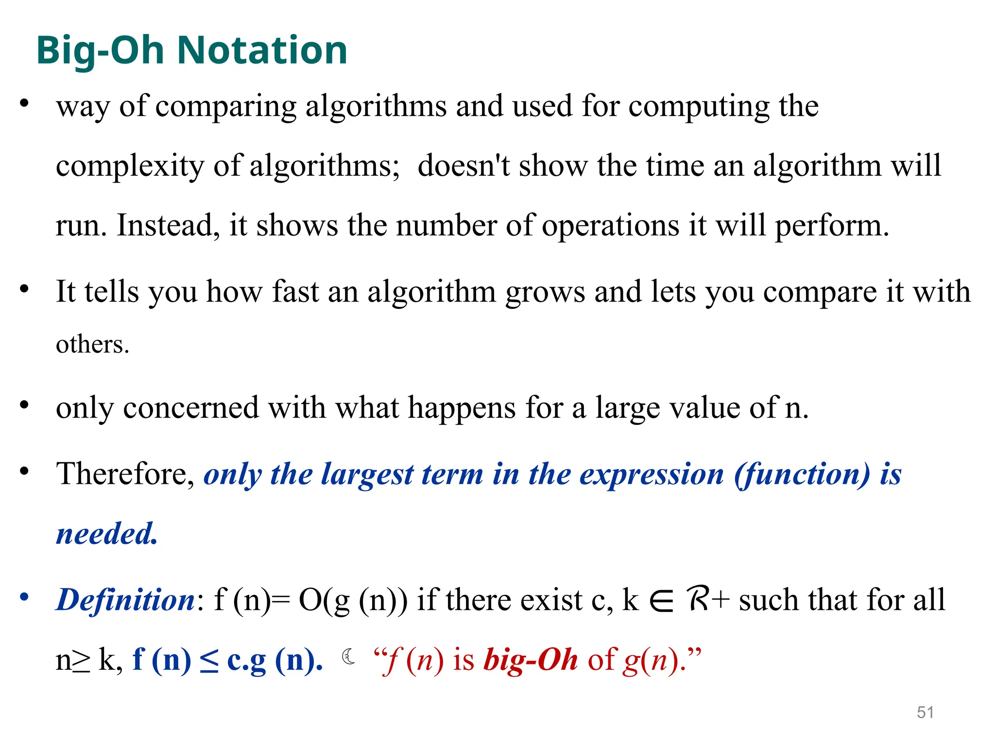
• way of comparing algorithms and used for computing the
complexity of algorithms; doesn't show the time an algorithm will
run. Instead, it shows the number of operations it will perform.
• It tells you how fast an algorithm grows and lets you compare it with
others.
• only concerned with what happens for a large value of n.
• Therefore, only the largest term in the expression (function) is
needed.
• Definition: f (n)= O(g (n)) if there exist c, k + such that for all
∊ ℛ
n≥ k, f (n) ≤ c.g (n).  “f (n) is big-Oh of g(n).”
51

52. Big-Oh Notation
Void fun(int n){
int i,j;
for(i=1;i<=n; i++)
for(j=1;j<=n ; j++){
cout<<“hello”;
break; }}
52
Big O Notation is determined by
identifying the dominant operation in an
algorithm and expressing its time
complexity in terms of n, where n
represents the input size.
From this f(n)=o(n)
While if we remove break, f(n)=o(n^2)
Big Oh rules
- Drop lower order
- Drop constant factor

53. Big-Oh Notation
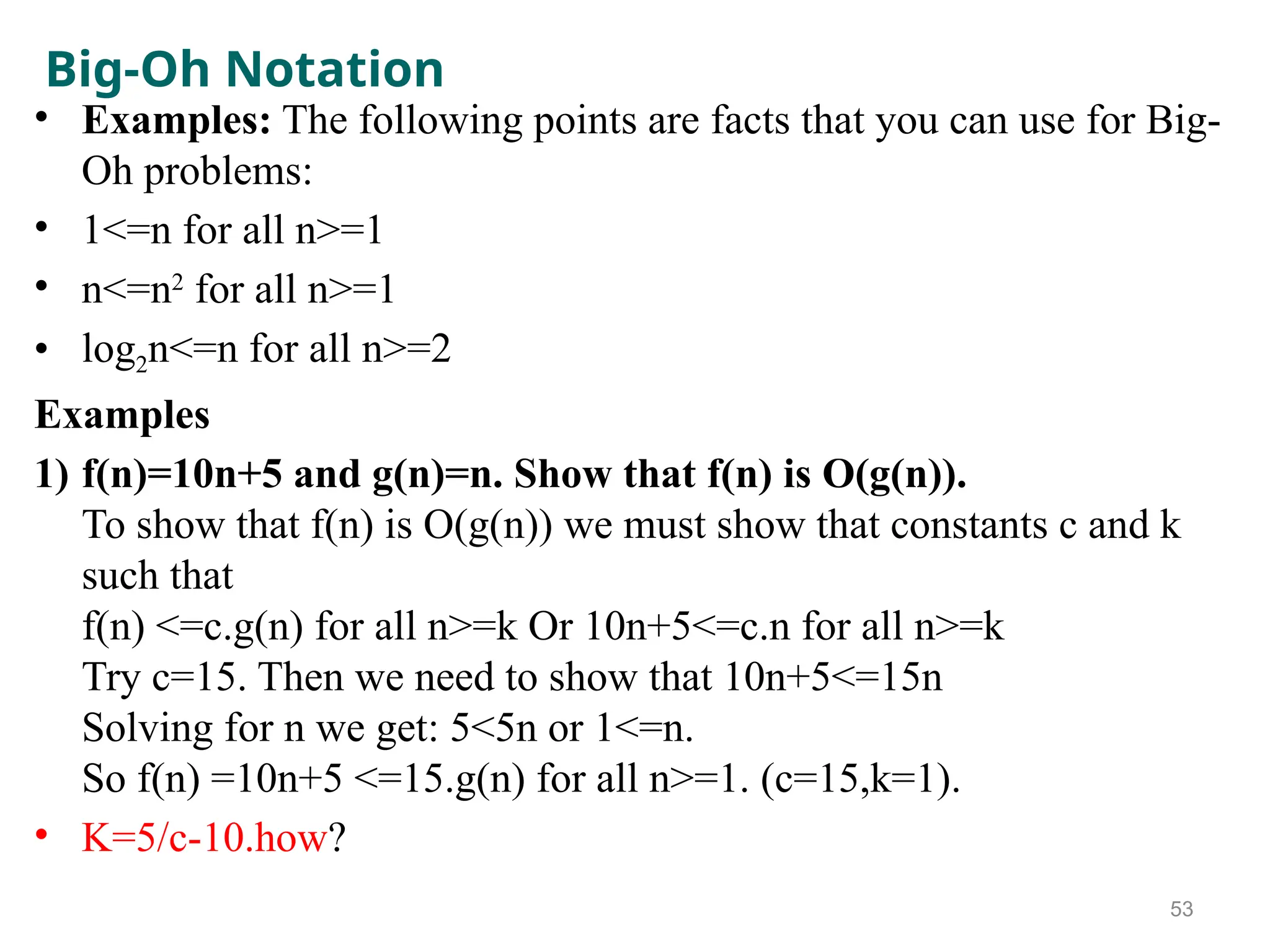
• Examples: The following points are facts that you can use for Big-
Oh problems:
• 1<=n for all n>=1
• n<=n2
for all n>=1
• log2n<=n for all n>=2
Examples
1) f(n)=10n+5 and g(n)=n. Show that f(n) is O(g(n)).
To show that f(n) is O(g(n)) we must show that constants c and k
such that
f(n) <=c.g(n) for all n>=k Or 10n+5<=c.n for all n>=k
Try c=15. Then we need to show that 10n+5<=15n
Solving for n we get: 5<5n or 1<=n.
So f(n) =10n+5 <=15.g(n) for all n>=1. (c=15,k=1).
• K=5/c-10.how?
53

54. The growth rate of this function is liner
54

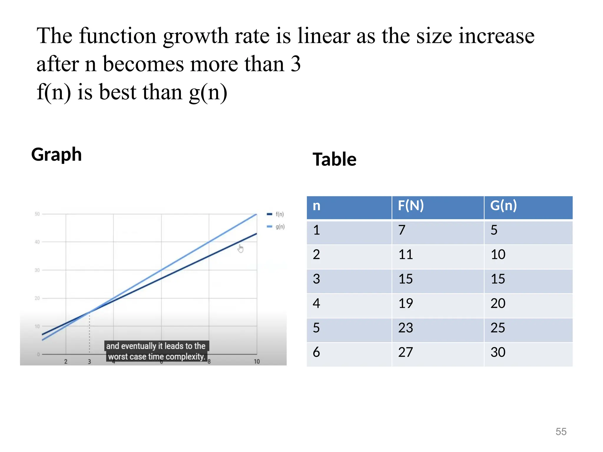
55. The function growth rate is linear as the size increase
after n becomes more than 3
f(n) is best than g(n)
Graph Table
n F(N) G(n)
1 7 5
2 11 10
3 15 15
4 19 20
5 23 25
6 27 30
55

56. Quadratic
56

57. Constant growth
57

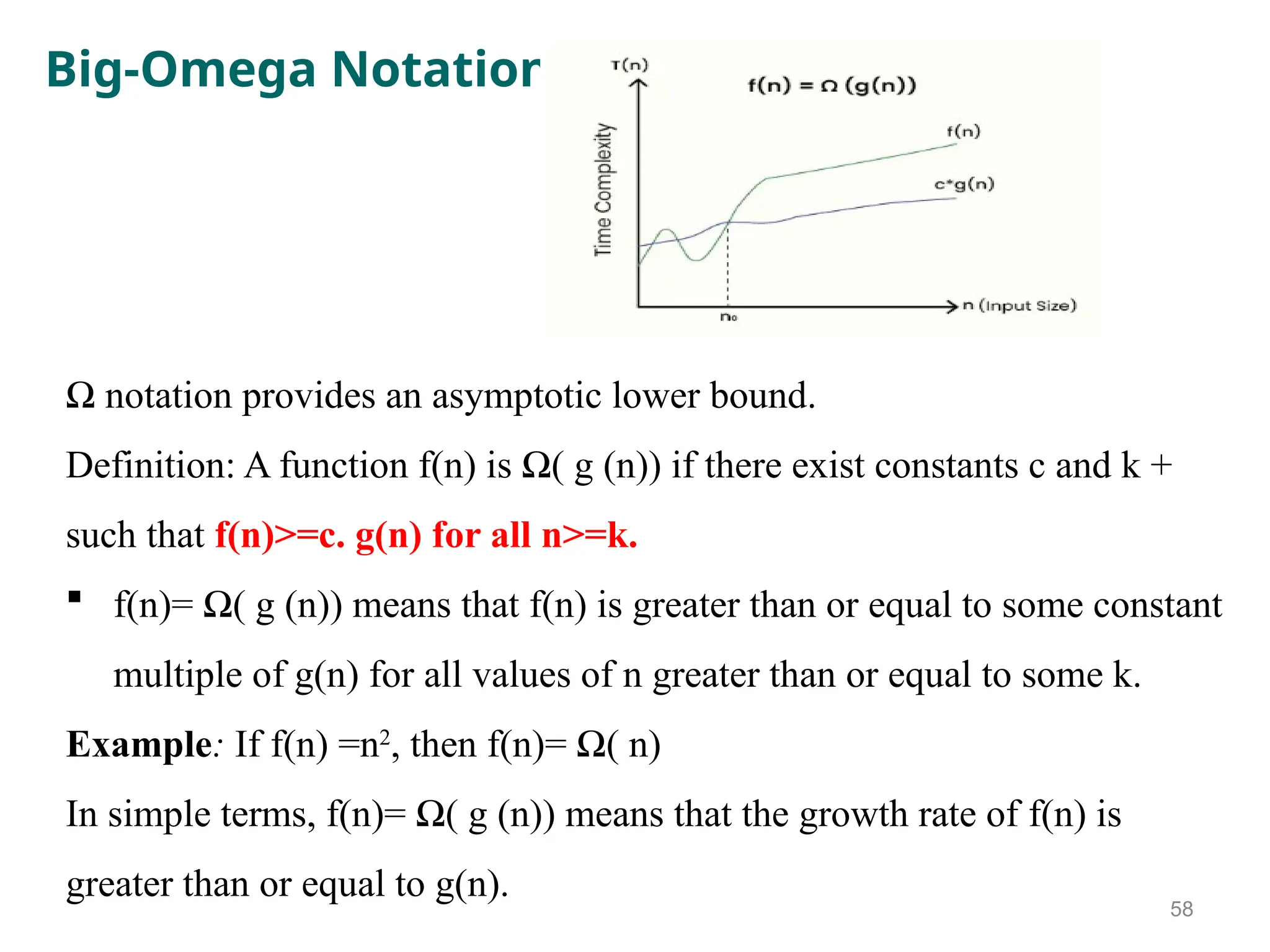
58. Big-Omega Notation
Ω notation provides an asymptotic lower bound.
Definition: A function f(n) is Ω( g (n)) if there exist constants c and k +
such that f(n)>=c. g(n) for all n>=k.
 f(n)= Ω( g (n)) means that f(n) is greater than or equal to some constant
multiple of g(n) for all values of n greater than or equal to some k.
Example: If f(n) =n2
, then f(n)= Ω( n)
In simple terms, f(n)= Ω( g (n)) means that the growth rate of f(n) is
greater than or equal to g(n).
58

59. Big-Omega Notation
59
Example: Let's take the function f(n) = 4n + 3and g(n) = n . Now we
need to see whether we can say f(n) = Ω(g(n)) .

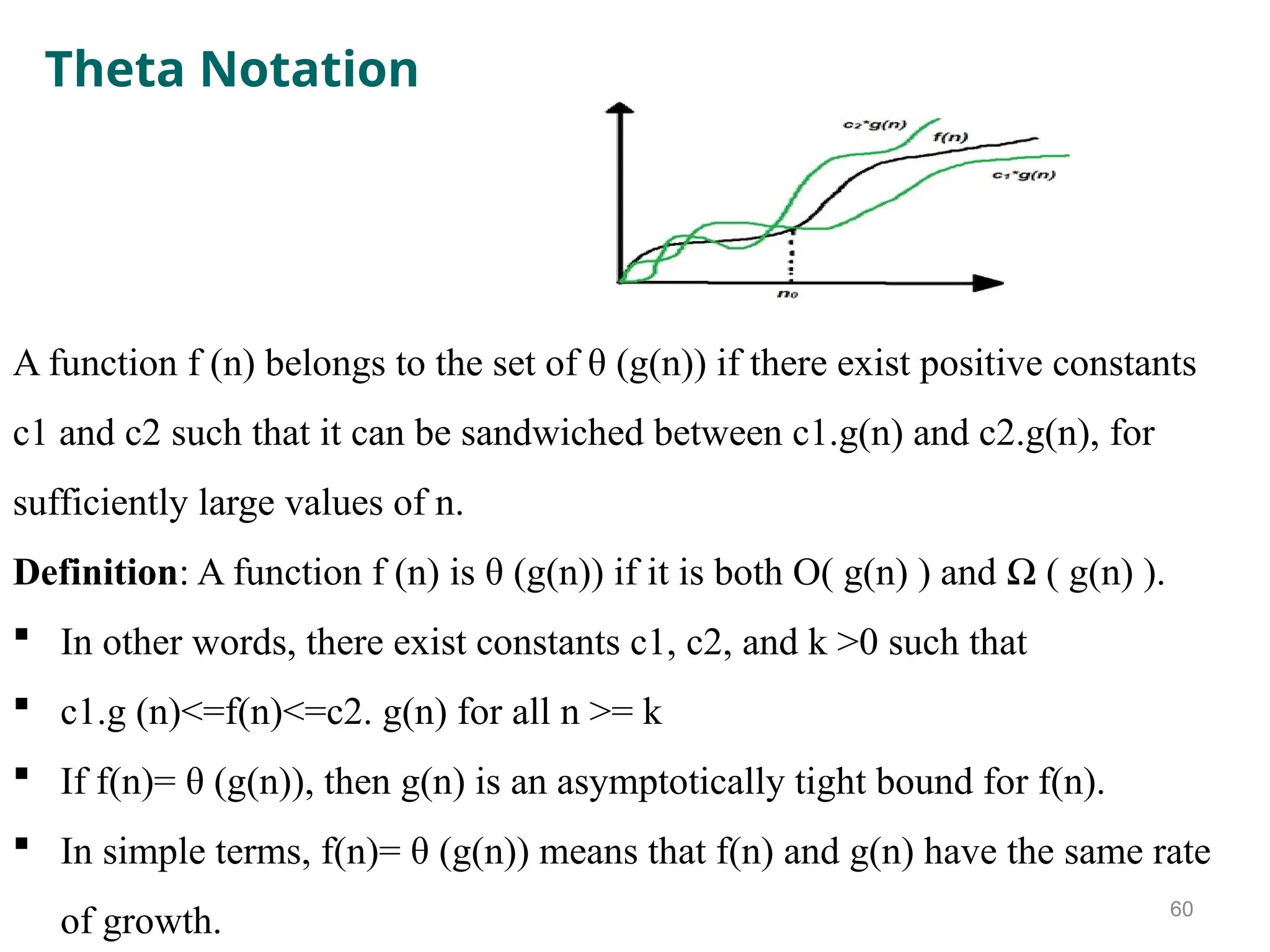
60. Theta Notation
A function f (n) belongs to the set of θ (g(n)) if there exist positive constants
c1 and c2 such that it can be sandwiched between c1.g(n) and c2.g(n), for
sufficiently large values of n.
Definition: A function f (n) is θ (g(n)) if it is both O( g(n) ) and Ω ( g(n) ).
 In other words, there exist constants c1, c2, and k >0 such that
 c1.g (n)<=f(n)<=c2. g(n) for all n >= k
 If f(n)= θ (g(n)), then g(n) is an asymptotically tight bound for f(n).
 In simple terms, f(n)= θ (g(n)) means that f(n) and g(n) have the same rate
of growth. 60

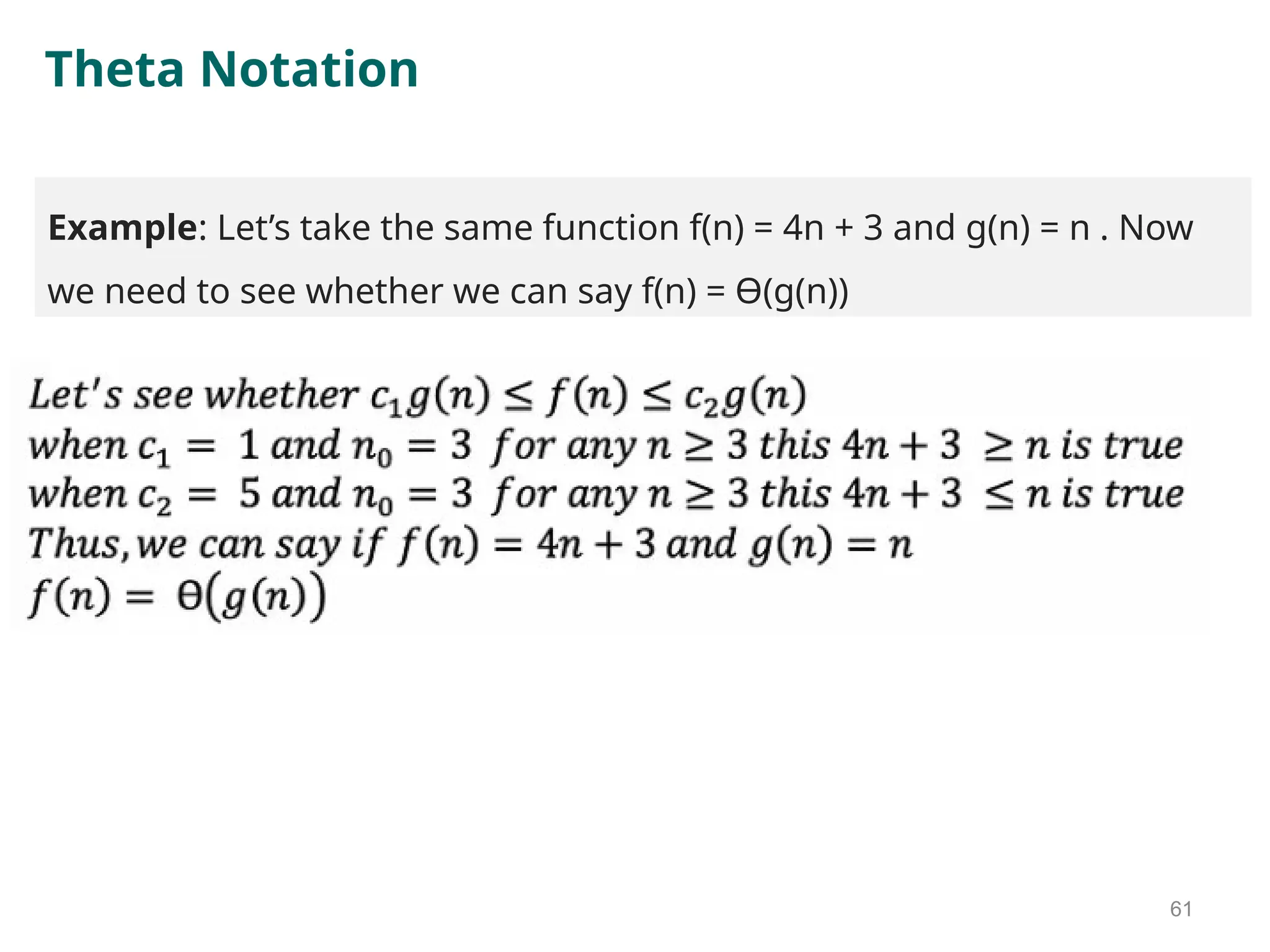
61. Theta Notation
61
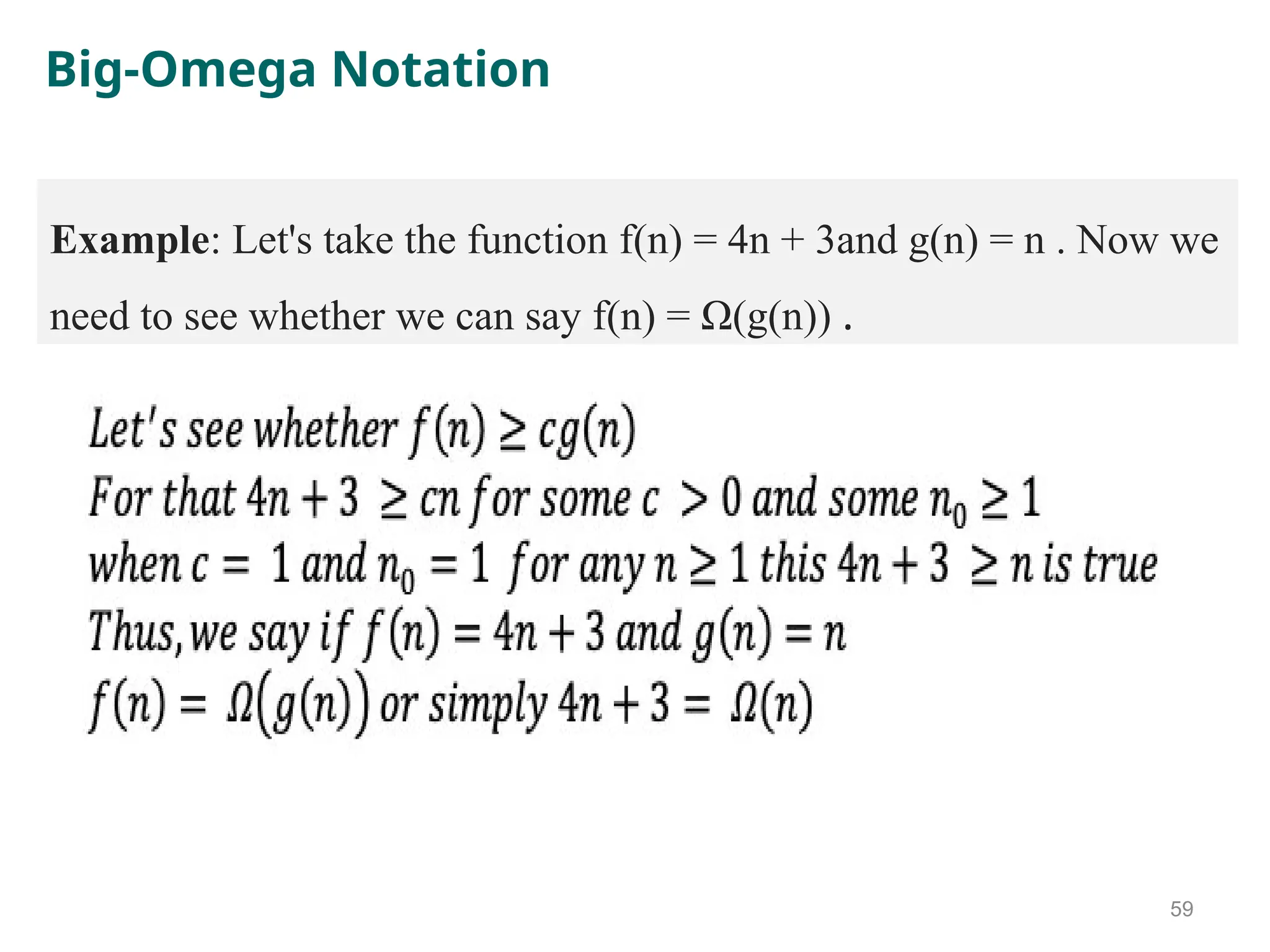
Example: Let’s take the same function f(n) = 4n + 3 and g(n) = n . Now
we need to see whether we can say f(n) = Ө(g(n))

62. Asymptotic Notations
Notations used to express the asymptotic behavior of the given function
62

63. Common time and space complexity classes
63

64. THANK YOU
64