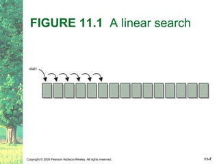
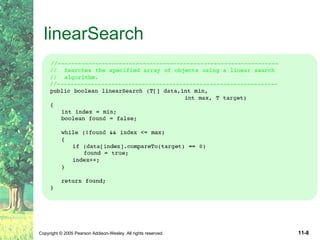
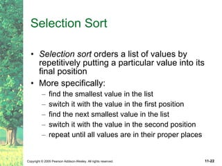
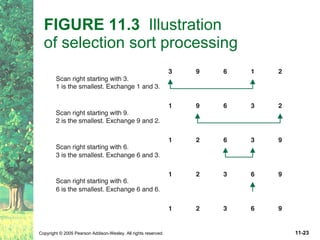
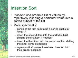
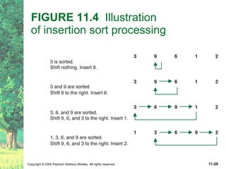
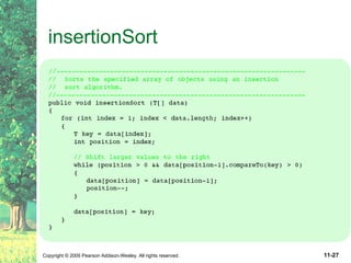
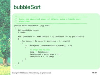
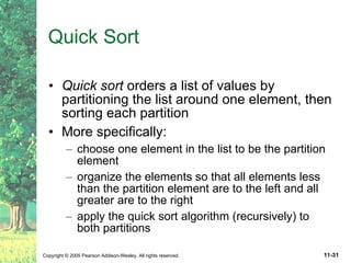
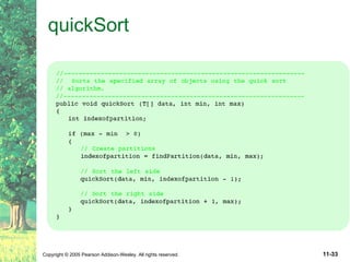
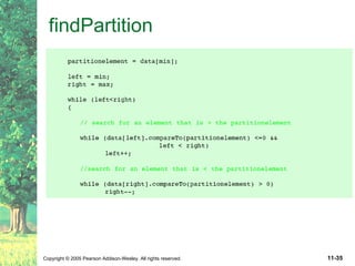
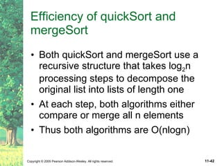
Chapter 11 Sorting  and Searching
Chapter Objectives Examine the linear search and binary search algorithms Examine several (vài)  sorting algorithms, including: selection sort insertion sort bubble sort quick sort merge sort Discuss the complexity (phức tạp)  of these algorithms
Searching Searching  is the process of finding a  target element  among a group of items (the  search pool ), or determining that it isn't there This requires repetitively comparing the target to candidates in the search pool An efficient sort performs no more comparisons than it has to The size of the search pool is a factor
The Comparable Interface We want to define the algorithms such that they can search any set of objects Therefore we will search objects that implement the  Comparable  interface It contains one method,  compareTo , which is designed to return an integer that specifies the relationship between two objects: obj1.compareTo(obj2) This call returns a number less than, equal to, or greater than 0 if  obj1  is less than, equal to, or greater than  obj2 , respectively
The Comparable Interface All of the methods presented in this chapter are part of the SortingandSearching class This class makes use of the generic type T For this class, we make the further distinction (khác biệt)  that T extends Comparable public class SortingandSearching<T extends Comparable>
Linear Search A  linear search  simply examines each item in the search pool, one at a time, until either the target is found or until the pool is exhausted This approach does not assume the items in the search pool are in any particular order We just need to be able to examine each element in turn (in a linear fashion) It's fairly easy to understand, but not very efficient
FIGURE 11.1  A linear search
linearSearch
 
Binary Search If the search pool is sorted, then we can be more efficient than a linear search A  binary search  eliminates large parts of the search pool with each comparison Instead of starting the search at one end, we begin in the middle If the target isn't found, we know that if it is in the pool at all, it is in one half or the other We can then jump to the middle of that half, and continue similarly
FIGURE 11.2  A binary search
Binary Search For example, find the number 29 in the following sorted list of numbers: 8  15  22  29  36  54  55  61  70  73  88 Compare the target to the middle value 54 We now know that if 29 is in the list, it is in the front half of the list With one comparison, we've eliminated half of the data Then compare to 22, eliminating another quarter of the data, etc.
Binary Search A binary search algorithm is often implemented recursively Each recursive call searches a smaller portion of the search pool The base case of the recursion is running out of  viable candidates  to search, which means the target is not in the search pool At any point there may be two &quot;middle&quot; values, in which case either could be used
binarySearch
Comparing Search Algorithms On average, a linear search would examine n/2 elements before finding the target Therefore, a linear search is O(n) The worst case for a binary search is (log 2 n) comparisons A binary search is a  logarithmic algorithm It has a time complexity of O(log 2 n) But keep in mind that the search pool must be sorted For large n, a binary search is much faster
Sorting Sorting  is the process of arranging a group of items into a defined order based on particular criteria Many sorting algorithms have been designed Sequential sorts  require approximately n 2  comparisons to sort n elements Logarithmic sorts  typically require nlog 2 n comparisons to sort n elements
Sorting Let's define a generic sorting problem that any of our sorting algorithms could help solve As with searching, we must be able to compare one element to another
Listing 11.1
Listing 11.1  (cont.)
Listing 11.2
Listing 11.2  (cont.)
Selection Sort Selection sort  orders a list of values by repetitively putting a particular value into its final position More specifically: find the smallest value in the list switch it with the value in the first position find the next smallest value in the list switch it with the value in the second position repeat until all values are in their proper places
FIGURE 11.3   Illustration  of selection sort processing
selectionSort
Insertion Sort Insertion sort  orders a list of values by repetitively inserting a particular value into a sorted subset of the list More specifically: consider the first item to be a sorted sublist of length 1 insert the second item into the sorted sublist, shifting the first item if needed insert the third item into the sorted sublist, shifting the other items as needed repeat until all values have been inserted into their proper positions
FIGURE 11.4   Illustration  of insertion sort processing
insertionSort
Bubble Sort Bubble sort  orders a list of values by repetitively comparing neighboring elements and swapping their positions if necessary More specifically: scan the list, exchanging adjacent elements if they are not in relative order; this bubbles the highest value to the top scan the list again, bubbling up the second highest value repeat until all elements have been placed in their proper order
bubbleSort
Comparing Sorts We've seen three sorts so far: selection sort insertion sort bubble sort They all use nested loops and perform approximately n 2  comparisons They are relatively inefficient Now we will turn our attention to more efficient sorts
Quick Sort Quick sort  orders a list of values by partitioning the list around one element, then sorting each partition More specifically: choose one element in the list to be the partition element organize the elements so that all elements less than the partition element are to the left and all greater are to the right apply the quick sort algorithm (recursively) to both partitions
Quick Sort The choice of the partition element is arbitrary For efficiency, it would be nice if the partition element divided the list roughly in half The algorithm will work in any case, however We will divide the work into two methods: quickSort  – performs the recursive algorithm findPartition  – rearranges the elements into two partitions
quickSort
findPartition
findPartition
findPartition
Merge Sort Merge sort  orders a list of values by recursively dividing the list in half until each sub-list has one element, then recombining More specifically: divide the list into two roughly equal parts recursively divide each part in half, continuing until a part contains only one element merge the two parts into one sorted list continue to merge parts as the recursion unfolds
FIGURE 11.5   The decomposition of merge sort
FIGURE 11.6  The merge portion  of the merge sort algorithm
mergeSort
mergeSort
Efficiency of quickSort and mergeSort Both quickSort and mergeSort use a recursive structure that takes log 2 n processing steps to decompose the original list into lists of length one At each step, both algorithms either compare or merge all n elements Thus both algorithms are O(nlogn)

Ch05 Black Jack

  • 1.
    Chapter 11 Sorting and Searching
  • 2.
    Chapter Objectives Examinethe linear search and binary search algorithms Examine several (vài) sorting algorithms, including: selection sort insertion sort bubble sort quick sort merge sort Discuss the complexity (phức tạp) of these algorithms
  • 3.
    Searching Searching is the process of finding a target element among a group of items (the search pool ), or determining that it isn't there This requires repetitively comparing the target to candidates in the search pool An efficient sort performs no more comparisons than it has to The size of the search pool is a factor
  • 4.
    The Comparable InterfaceWe want to define the algorithms such that they can search any set of objects Therefore we will search objects that implement the Comparable interface It contains one method, compareTo , which is designed to return an integer that specifies the relationship between two objects: obj1.compareTo(obj2) This call returns a number less than, equal to, or greater than 0 if obj1 is less than, equal to, or greater than obj2 , respectively
  • 5.
    The Comparable InterfaceAll of the methods presented in this chapter are part of the SortingandSearching class This class makes use of the generic type T For this class, we make the further distinction (khác biệt) that T extends Comparable public class SortingandSearching<T extends Comparable>
  • 6.
    Linear Search A linear search simply examines each item in the search pool, one at a time, until either the target is found or until the pool is exhausted This approach does not assume the items in the search pool are in any particular order We just need to be able to examine each element in turn (in a linear fashion) It's fairly easy to understand, but not very efficient
  • 7.
    FIGURE 11.1 A linear search
  • 8.
  • 9.
  • 10.
    Binary Search Ifthe search pool is sorted, then we can be more efficient than a linear search A binary search eliminates large parts of the search pool with each comparison Instead of starting the search at one end, we begin in the middle If the target isn't found, we know that if it is in the pool at all, it is in one half or the other We can then jump to the middle of that half, and continue similarly
  • 11.
    FIGURE 11.2 A binary search
  • 12.
    Binary Search Forexample, find the number 29 in the following sorted list of numbers: 8 15 22 29 36 54 55 61 70 73 88 Compare the target to the middle value 54 We now know that if 29 is in the list, it is in the front half of the list With one comparison, we've eliminated half of the data Then compare to 22, eliminating another quarter of the data, etc.
  • 13.
    Binary Search Abinary search algorithm is often implemented recursively Each recursive call searches a smaller portion of the search pool The base case of the recursion is running out of viable candidates to search, which means the target is not in the search pool At any point there may be two &quot;middle&quot; values, in which case either could be used
  • 14.
  • 15.
    Comparing Search AlgorithmsOn average, a linear search would examine n/2 elements before finding the target Therefore, a linear search is O(n) The worst case for a binary search is (log 2 n) comparisons A binary search is a logarithmic algorithm It has a time complexity of O(log 2 n) But keep in mind that the search pool must be sorted For large n, a binary search is much faster
  • 16.
    Sorting Sorting is the process of arranging a group of items into a defined order based on particular criteria Many sorting algorithms have been designed Sequential sorts require approximately n 2 comparisons to sort n elements Logarithmic sorts typically require nlog 2 n comparisons to sort n elements
  • 17.
    Sorting Let's definea generic sorting problem that any of our sorting algorithms could help solve As with searching, we must be able to compare one element to another
  • 18.
  • 19.
  • 20.
  • 21.
  • 22.
    Selection Sort Selectionsort orders a list of values by repetitively putting a particular value into its final position More specifically: find the smallest value in the list switch it with the value in the first position find the next smallest value in the list switch it with the value in the second position repeat until all values are in their proper places
  • 23.
    FIGURE 11.3 Illustration of selection sort processing
  • 24.
  • 25.
    Insertion Sort Insertionsort orders a list of values by repetitively inserting a particular value into a sorted subset of the list More specifically: consider the first item to be a sorted sublist of length 1 insert the second item into the sorted sublist, shifting the first item if needed insert the third item into the sorted sublist, shifting the other items as needed repeat until all values have been inserted into their proper positions
  • 26.
    FIGURE 11.4 Illustration of insertion sort processing
  • 27.
  • 28.
    Bubble Sort Bubblesort orders a list of values by repetitively comparing neighboring elements and swapping their positions if necessary More specifically: scan the list, exchanging adjacent elements if they are not in relative order; this bubbles the highest value to the top scan the list again, bubbling up the second highest value repeat until all elements have been placed in their proper order
  • 29.
  • 30.
    Comparing Sorts We'veseen three sorts so far: selection sort insertion sort bubble sort They all use nested loops and perform approximately n 2 comparisons They are relatively inefficient Now we will turn our attention to more efficient sorts
  • 31.
    Quick Sort Quicksort orders a list of values by partitioning the list around one element, then sorting each partition More specifically: choose one element in the list to be the partition element organize the elements so that all elements less than the partition element are to the left and all greater are to the right apply the quick sort algorithm (recursively) to both partitions
  • 32.
    Quick Sort Thechoice of the partition element is arbitrary For efficiency, it would be nice if the partition element divided the list roughly in half The algorithm will work in any case, however We will divide the work into two methods: quickSort – performs the recursive algorithm findPartition – rearranges the elements into two partitions
  • 33.
  • 34.
  • 35.
  • 36.
  • 37.
    Merge Sort Mergesort orders a list of values by recursively dividing the list in half until each sub-list has one element, then recombining More specifically: divide the list into two roughly equal parts recursively divide each part in half, continuing until a part contains only one element merge the two parts into one sorted list continue to merge parts as the recursion unfolds
  • 38.
    FIGURE 11.5 The decomposition of merge sort
  • 39.
    FIGURE 11.6 The merge portion of the merge sort algorithm
  • 40.
  • 41.
  • 42.
    Efficiency of quickSortand mergeSort Both quickSort and mergeSort use a recursive structure that takes log 2 n processing steps to decompose the original list into lists of length one At each step, both algorithms either compare or merge all n elements Thus both algorithms are O(nlogn)