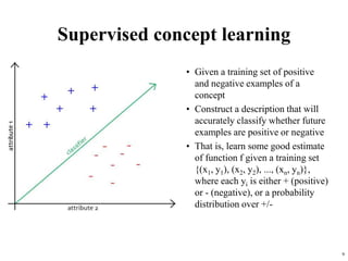
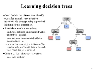
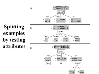
The document summarizes material from a machine learning class. It defines machine learning as using examples to reach general conclusions and make predictions. It describes supervised learning, where examples are labeled, and unsupervised learning, which only uses inputs. Decision trees are discussed as a method that partitions data into regions to classify it.

1. 1
CMSC 671
Fall 2010
Class #23 — Monday, November 22

2. 2
Today’s class
• Machine learning
– What is ML?
– Inductive learning
• Supervised
• Unsupervised
– Decision trees
• Later we’ll also cover:
– Other classification methods (k-nearest neighbor, naïve Bayes, BN
learning, support vector machines, neural nets)
– Clustering

3. 3
Machine Learning
Chapter 18.1-18.4
Some material adopted from notes
by Chuck Dyer

4. 4
What is learning?
• “Learning denotes changes in a system that ...
enable a system to do the same task more
efficiently the next time.” –Herbert Simon
• “Learning is constructing or modifying
representations of what is being experienced.”
–Ryszard Michalski
• “Learning is making useful changes in our minds.”
–Marvin Minsky

5. 5
Why learn?
• Understand and improve efficiency of human learning
– Use to improve methods for teaching and tutoring people (e.g., better
computer-aided instruction)
• Discover new things or structure that were previously
unknown to humans
– Examples: data mining, scientific discovery
• Fill in skeletal or incomplete specifications about a domain
– Large, complex AI systems cannot be completely derived by hand
and require dynamic updating to incorporate new information.
– Learning new characteristics expands the domain or expertise and
lessens the “brittleness” of the system
• Build software agents that can adapt to their users or to
other software agents

6. 6
A general model of learning agents

7. 7
Major paradigms of machine learning
• Rote learning – One-to-one mapping from inputs to stored
representation. “Learning by memorization.” Association-based
storage and retrieval.
• Induction – Use specific examples to reach general conclusions
– Classification – Predict one of a discrete set of labels
– Regression – Predict a continuous class value
• Clustering – Unsupervised identification of natural groups in data
• Analogy – Determine correspondence between two different
representations
• Discovery – Unsupervised, specific goal not given
• Genetic algorithms – “Evolutionary” search techniques, based on
an analogy to “survival of the fittest”
• Reinforcement – Feedback (positive or negative reward) given at
the end of a sequence of steps

8. 8
The classification problem
• Extrapolate from a given set of examples
to make accurate predictions about future
examples
• Supervised versus unsupervised learning
– Learn an unknown function f(X) = Y,
where X is an input example and Y is the
desired output.
– Supervised learning implies we are
given a training set of (X, Y) pairs by a
“teacher”
– Unsupervised learning means we are
only given the Xs and some (ultimate)
feedback function on our performance.
• Concept learning or classification
–Given a set of examples of some concept/class/category, determine if a given
example is an instance of the concept or not
–If it is an instance, we call it a positive example
–If it is not, it is called a negative example
–Or we can make a probabilistic prediction (e.g., using a Bayes net)

9. 9
Supervised concept learning
• Given a training set of positive
and negative examples of a
concept
• Construct a description that will
accurately classify whether future
examples are positive or negative
• That is, learn some good estimate
of function f given a training set
{(x1, y1), (x2, y2), ..., (xn, yn)},
where each yi is either + (positive)
or - (negative), or a probability
distribution over +/-

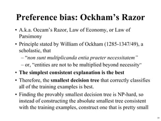
10. 10
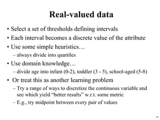
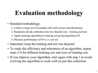
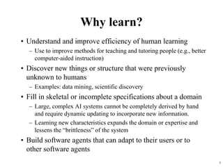
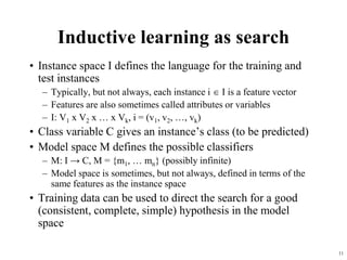
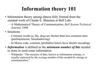
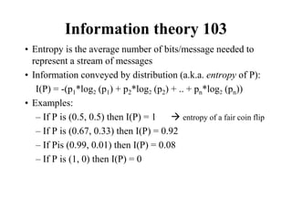
Inductive learning framework
• Raw input data from sensors are typically
preprocessed to obtain a feature vector, X,
that adequately describes all of the relevant
features for classifying examples
• Each x is a list of (attribute, value) pairs. For
example,
X = [Person:Sue, EyeColor:Brown, Age:Young,
Sex:Female]
• The number of attributes (a.k.a. features) is
fixed (positive, finite)
• Each attribute has a fixed, finite number of
possible values (or could be continuous)
• Each example can be interpreted as a point in an
n-dimensional feature space, where n is the number of attributes

11. 11
Inductive learning as search
• Instance space I defines the language for the training and
test instances
– Typically, but not always, each instance i  I is a feature vector
– Features are also sometimes called attributes or variables
– I: V1 x V2 x … x Vk, i = (v1, v2, …, vk)
• Class variable C gives an instance’s class (to be predicted)
• Model space M defines the possible classifiers
– M: I → C, M = {m1, … mn} (possibly infinite)
– Model space is sometimes, but not always, defined in terms of the
same features as the instance space
• Training data can be used to direct the search for a good
(consistent, complete, simple) hypothesis in the model
space

12. 12
Model spaces
• Decision trees
– Partition the instance space into axis-parallel regions, labeled with class
value
• Version spaces
– Search for necessary (lower-bound) and sufficient (upper-bound) partial
instance descriptions for an instance to be in the class
• Nearest-neighbor classifiers
– Partition the instance space into regions defined by the centroid instances
(or cluster of k instances)
• Bayesian networks (probabilistic dependencies of class on attributes)
– Naïve Bayes: special case of BNs where class  each attribute
• Neural networks
– Nonlinear feed-forward functions of attribute values
• Support vector machines
– Find a separating plane in a high-dimensional feature space
• Associative rules (feature values → class)
• First-order logical rules

13. 13
Model spaces I
+
+
-
-
I
+
+
-
-
I
+
+
-
-
Nearest
neighbor
Version space
Decision
tree

14. 14
Learning decision trees
•Goal: Build a decision tree to classify
examples as positive or negative
instances of a concept using supervised
learning from a training set
•A decision tree is a tree where
– each non-leaf node has associated with it
an attribute (feature)
–each leaf node has associated with it a
classification (+ or -)
–each arc has associated with it one of the
possible values of the attribute at the node
from which the arc is directed
•Generalization: allow for >2 classes
–e.g., {sell, hold, buy}

15. 15
Decision tree-induced partition – example
I

16. Expressiveness
• Decision trees can express any function of the input attributes.
• E.g., for Boolean functions, truth table row → path to leaf:
• Trivially, there is a consistent decision tree for any training set with one
path to leaf for each example (unless f nondeterministic in x) but it
probably won't generalize to new examples
• We prefer to find more compact decision trees

17. Inductive learning and bias
• Suppose that we want to learn a function f(x) = y and we
are given some sample (x,y) pairs, as in figure (a)
• There are several hypotheses we could make about this
function, e.g.: (b), (c) and (d)
• A preference for one over the others reveals the bias of our
learning technique, e.g.:
– prefer piece-wise functions (b)
– prefer a smooth function (c)
– prefer a simple function and treat outliers as noise (d)

18. 18
Preference bias: Ockham’s Razor
• A.k.a. Occam’s Razor, Law of Economy, or Law of
Parsimony
• Principle stated by William of Ockham (1285-1347/49), a
scholastic, that
– “non sunt multiplicanda entia praeter necessitatem”
– or, “entities are not to be multiplied beyond necessity”
• The simplest consistent explanation is the best
• Therefore, the smallest decision tree that correctly classifies
all of the training examples is best.
• Finding the provably smallest decision tree is NP-hard, so
instead of constructing the absolute smallest tree consistent
with the training examples, construct one that is pretty small

19. 19
R&N’s restaurant domain
• Develop a decision tree to model the decision a patron
makes when deciding whether or not to wait for a table at a
restaurant
• Two classes: wait, leave
• Ten attributes: Alternative available? Bar in restaurant? Is it
Friday? Are we hungry? How full is the restaurant? How
expensive? Is it raining? Do we have a reservation? What
type of restaurant is it? What’s the purported waiting time?
• Training set of 12 examples
• ~ 7000 possible cases

20. 20
A decision tree
from introspection

21. 21
A training set

22. 22
ID3 / C4.5
• A greedy algorithm for decision tree construction developed
by Ross Quinlan, 1987
• Top-down construction of the decision tree by recursively
selecting the “best attribute” to use at the current node in the
tree
– Once the attribute is selected for the current node,
generate children nodes, one for each possible value of
the selected attribute
– Partition the examples using the possible values of this
attribute, and assign these subsets of the examples to the
appropriate child node
– Repeat for each child node until all examples associated
with a node are either all positive or all negative

23. 23
Choosing the best attribute
• The key problem is choosing which attribute to split a given
set of examples
• Some possibilities are:
– Random: Select any attribute at random
– Least-Values: Choose the attribute with the smallest number of
possible values
– Most-Values: Choose the attribute with the largest number of
possible values
– Max-Gain: Choose the attribute that has the largest expected
information gain–i.e., the attribute that will result in the smallest
expected size of the subtrees rooted at its children
• The ID3 algorithm uses the Max-Gain method of selecting
the best attribute

24. Choosing an attribute
Idea: a good attribute splits the examples into subsets
that are (ideally) “all positive” or “all negative”
Which is better: Patrons? or Type?

25. 25
Restaurant example
French
Italian
Thai
Burger
Empty Some Full
Y
Y
Y
Y
Y
Y
N
N
N
N
N
N
Random: Patrons or Wait-time; Least-values: Patrons; Most-values: Type; Max-gain: ???

26. 26
Splitting
examples
by testing
attributes

27. 27
ID3-induced
decision tree

28. Information theory 101
• Information theory sprang almost fully formed from the
seminal work of Claude E. Shannon at Bell Labs
– A Mathematical Theory of Communication, Bell System Technical
Journal, 1948.
• Intuitions
– Common words (a, the, dog) are shorter than less common ones
(parlimentarian, foreshadowing)
– In Morse code, common (probable) letters have shorter encodings
• Information is defined as the minimum number of bits needed
to store or send some information
– Wikipedia: “The measure of data, known as information entropy, is
usually expressed by the average number of bits needed for storage or
communication.”

29. Information theory 102
• Information is measured in bits
• Information conveyed by a message depends on its probability
• With n equally probable possible messages, the probability p
of each is 1/n
• Information conveyed by message is log2(n)
– e.g., with 16 messages, then log2 (16) = 4 and we need 4
bits to identify/send each message
• Given probability distribution for n messages P = (p1,p2…pn),
the information conveyed by distribution (aka entropy of P)
is:
I(P) = -(p1*log2 (p1) + p2*log2 (p2) + .. + pn*log2 (pn))
info in msg 2
probability of msg 2

30. Information theory 103
• Entropy is the average number of bits/message needed to
represent a stream of messages
• Information conveyed by distribution (a.k.a. entropy of P):
I(P) = -(p1*log2 (p1) + p2*log2 (p2) + .. + pn*log2 (pn))
• Examples:
– If P is (0.5, 0.5) then I(P) = 1  entropy of a fair coin flip
– If P is (0.67, 0.33) then I(P) = 0.92
– If Pis (0.99, 0.01) then I(P) = 0.08
– If P is (1, 0) then I(P) = 0

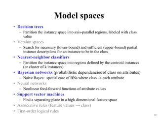
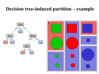
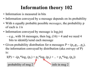
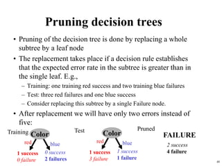
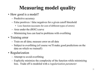
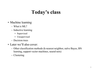
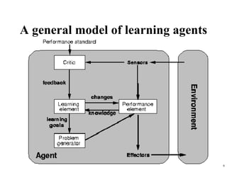
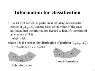
31. Entropy as measure of homogeneity of
examples
• Entropy used to characterize the (im)purity of an arbitrary
collection of examples.
• Given a collection S (e.g. the table with 12 examples for the
restaurant domain), containing positive and negative
examples of some target concept, the entropy of S relative
to its boolean classification is:
I(S) = -(p+*log2 (p+) + p-*log2 (p-))
Entropy([6+, 6-]) = 1  entropy of the restaurant dataset
Entropy([9+, 5-]) = 0.940

32. 34
Information for classification
• If a set T of records is partitioned into disjoint exhaustive
classes (C1,C2,..,Ck) on the basis of the value of the class
attribute, then the information needed to identify the class of
an element of T is
Info(T) = I(P)
where P is the probability distribution of partition (C1,C2,..,Ck):
P = (|C1|/|T|, |C2|/|T|, ..., |Ck|/|T|)
C1
C2
C3
C1
C2
C3
High information
Low information

33. 35
Information for classification II
• If we partition T w.r.t attribute X into sets {T1,T2, ..,Tn}
then the information needed to identify the class of an
element of T becomes the weighted average of the
information needed to identify the class of an element of Ti,
i.e. the weighted average of Info(Ti):
Info(X,T) = S|Ti|/|T| * Info(Ti)
C1
C2
C3
C1
C2
C3
High information Low information

34. Information gain
• A chosen attribute A divides the training set E into subsets E1, … , Ev
according to their values for A, where A has v distinct values.
• The quantity IG(S,A), the information gain of an attribute A relative to a
collection of examples S, is defined as:
Gain(S,A) = I(S) – Remainder(A)
• This represents the difference between
– I(S) – the entropy of the original collection S
– Remainder(A) - expected value of the entropy after S is partitioned using
attribute A
• This is the gain in information due to attribute A
– Expected reduction in entropy
– IG(S,A) or simply IG(A):

 




v
i i
i
i
i
i
i
i
i
n
p
n
n
p
p
I
n
p
n
p
A
remainder
1
)
,
(
)
(
)
(
|
|
|
|
)
(
)
,
( )
( v
A
Values
v
v
S
I
S
S
S
I
A
S
IG 

 
)
(
)
,
(
)
( A
remainder
n
p
n
n
p
p
I
A
IG 




35. Information gain, cont.
• Use to rank attributes and build DT (decision tree)
where each node uses attribute with greatest gain of
those not yet considered (in path from root)
• The intent of this ordering is to:
– Create small DTs so records can be identified with few
questions
– Match a hoped-for minimality of the process represented
by the records being considered (Occam’s Razor)

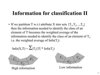
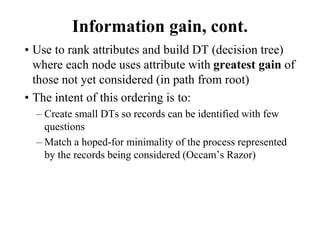
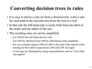
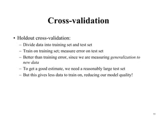
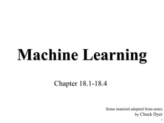
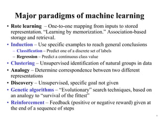
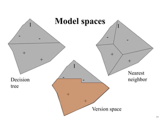
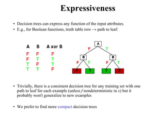
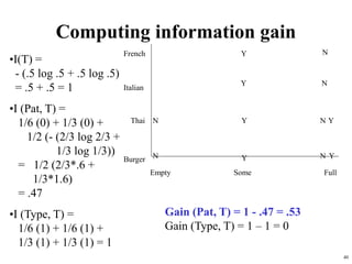
36. Information gain, cont.
For the training set, S:
p = n = 6,
I(6/12, 6/12) = 1 bit
Consider the attributes Patrons and Type (and others too):
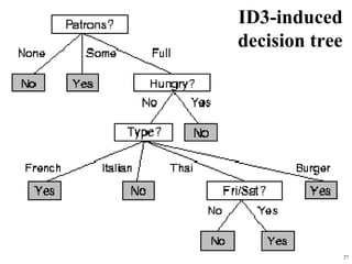
Patrons has the highest IG of all attributes and so is chosen by the DTL algorithm
as the root
bits
0
)]
4
2
,
4
2
(
12
4
)
4
2
,
4
2
(
12
4
)
2
1
,
2
1
(
12
2
)
2
1
,
2
1
(
12
2
[
1
)
(
bits
0541
.
)]
6
4
,
6
2
(
12
6
)
0
,
1
(
12
4
)
1
,
0
(
12
2
[
1
)
(











I
I
I
I
Type
IG
I
I
I
Patrons
IG

37. 39
Computing information gain
French
Italian
Thai
Burger
Empty Some Full
Y
Y
Y
Y
Y
Y
N
N
N
N
N
N
•I(T) = ?
•I (Pat, T) = ?
•I (Type, T) = ?
Gain (Pat, T) = ?
Gain (Type, T) = ?

38. 40
Computing information gain
French
Italian
Thai
Burger
Empty Some Full
Y
Y
Y
Y
Y
Y
N
N
N
N
N
N
•I(T) =
- (.5 log .5 + .5 log .5)
= .5 + .5 = 1
•I (Pat, T) =
1/6 (0) + 1/3 (0) +
1/2 (- (2/3 log 2/3 +
1/3 log 1/3))
= 1/2 (2/3*.6 +
1/3*1.6)
= .47
•I (Type, T) =
1/6 (1) + 1/6 (1) +
1/3 (1) + 1/3 (1) = 1
Gain (Pat, T) = 1 - .47 = .53
Gain (Type, T) = 1 – 1 = 0

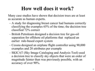
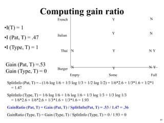
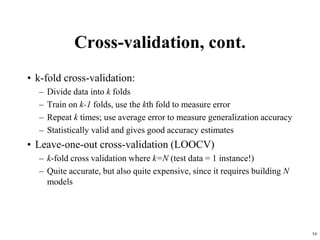
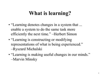
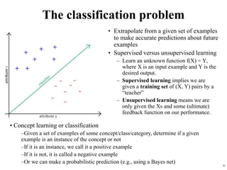
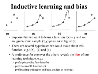
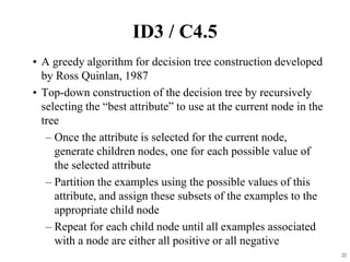
39. 41
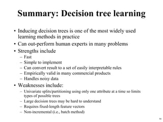
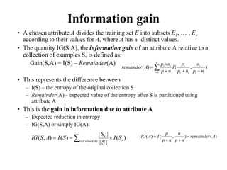
The ID3 algorithm is used to build a decision tree, given a set of non-categorical attributes
C1, C2, .., Cn, the class attribute C, and a training set T of records.
function ID3 (R: a set of input attributes,
C: the class attribute,
S: a training set) returns a decision tree;
begin
If S is empty, return a single node with value Failure;
If every example in S has the same value for C, return
single node with that value;
If R is empty, then return a single node with most
frequent of the values of C found in examples S;
[note: there will be errors, i.e., improperly classified
records];
Let D be attribute with largest Gain(D,S) among attributes in R;
Let {dj| j=1,2, .., m} be the values of attribute D;
Let {Sj| j=1,2, .., m} be the subsets of S consisting
respectively of records with value dj for attribute D;
Return a tree with root labeled D and arcs labeled
d1, d2, .., dm going respectively to the trees
ID3(R-{D},C,S1), ID3(R-{D},C,S2) ,.., ID3(R-{D},C,Sm);
end ID3;

40. 42
How well does it work?
Many case studies have shown that decision trees are at least
as accurate as human experts.
– A study for diagnosing breast cancer had humans correctly
classifying the examples 65% of the time; the decision tree
classified 72% correct
– British Petroleum designed a decision tree for gas-oil
separation for offshore oil platforms that replaced an
earlier rule-based expert system
– Cessna designed an airplane flight controller using 90,000
examples and 20 attributes per example
– SKICAT (Sky Image Cataloging and Analysis Tool) used
a decision tree to classify sky objects that were an order of
magnitude fainter than was previously possible, with an
accuracy of over 90%.

41. 43
Extensions of ID3
• Using gain ratios
• Real-valued data
• Noisy data and overfitting – pruning, early stopping,
windowing
• Generation of rules
• Setting parameters
• Cross-validation for experimental validation of performance
• C4.5 is an extension of ID3 that accounts for unavailable
values, continuous attribute value ranges, pruning of
decision trees, rule derivation, and so on

42. 44
Using gain ratios
• The information gain criterion favors attributes that have a large
number of values
– If we have an attribute D that has a distinct value for each
record, then Info(D,T) is 0, thus Gain(D,T) is maximal
• To compensate for this, Quinlan suggests using the following
ratio instead of Gain:
GainRatio(D,T) = Gain(D,T) / SplitInfo(D,T)
• SplitInfo(D,T) is the information due to the split of T on the
basis of value of categorical attribute D
SplitInfo(D,T) = I(|T1|/|T|, |T2|/|T|, .., |Tm|/|T|)
where {T1, T2, .. Tm} is the partition of T induced by value of D

43. 45
Computing gain ratio
French
Italian
Thai
Burger
Empty Some Full
Y
Y
Y
Y
Y
Y
N
N
N
N
N
N
•I(T) = 1
•I (Pat, T) = .47
•I (Type, T) = 1
Gain (Pat, T) =.53
Gain (Type, T) = 0
SplitInfo (Pat, T) = - (1/6 log 1/6 + 1/3 log 1/3 + 1/2 log 1/2) = 1/6*2.6 + 1/3*1.6 + 1/2*1
= 1.47
SplitInfo (Type, T) = 1/6 log 1/6 + 1/6 log 1/6 + 1/3 log 1/3 + 1/3 log 1/3
= 1/6*2.6 + 1/6*2.6 + 1/3*1.6 + 1/3*1.6 = 1.93
GainRatio (Pat, T) = Gain (Pat, T) / SplitInfo(Pat, T) = .53 / 1.47 = .36
GainRatio (Type, T) = Gain (Type, T) / SplitInfo (Type, T) = 0 / 1.93 = 0

44. 46
Real-valued data
• Select a set of thresholds defining intervals
• Each interval becomes a discrete value of the attribute
• Use some simple heuristics…
– always divide into quartiles
• Use domain knowledge…
– divide age into infant (0-2), toddler (3 - 5), school-aged (5-8)
• Or treat this as another learning problem
– Try a range of ways to discretize the continuous variable and
see which yield “better results” w.r.t. some metric
– E.g., try midpoint between every pair of values

45. 48
Pruning decision trees
• Pruning of the decision tree is done by replacing a whole
subtree by a leaf node
• The replacement takes place if a decision rule establishes
that the expected error rate in the subtree is greater than in
the single leaf. E.g.,
– Training: one training red success and two training blue failures
– Test: three red failures and one blue success
– Consider replacing this subtree by a single Failure node.
• After replacement we will have only two errors instead of
five:
Color
1 success
0 failure
0 success
2 failures
red blue
Color
1 success
3 failure
1 success
1 failure
red blue 2 success
4 failure
FAILURE
Training Test Pruned

46. 49
Converting decision trees to rules
• It is easy to derive a rule set from a decision tree: write a rule
for each path in the decision tree from the root to a leaf
• In that rule the left-hand side is easily built from the label of
the nodes and the labels of the arcs
• The resulting rules set can be simplified:
– Let LHS be the left hand side of a rule
– Let LHS' be obtained from LHS by eliminating some conditions
– We can certainly replace LHS by LHS' in this rule if the subsets of the
training set that satisfy respectively LHS and LHS' are equal
– A rule may be eliminated by using metaconditions such as “if no other
rule applies”

47. 50
Summary: Decision tree learning
• Inducing decision trees is one of the most widely used
learning methods in practice
• Can out-perform human experts in many problems
• Strengths include
– Fast
– Simple to implement
– Can convert result to a set of easily interpretable rules
– Empirically valid in many commercial products
– Handles noisy data
• Weaknesses include:
– Univariate splits/partitioning using only one attribute at a time so limits
types of possible trees
– Large decision trees may be hard to understand
– Requires fixed-length feature vectors
– Non-incremental (i.e., batch method)

48. 51
Evaluation methodology
• Standard methodology:
1. Collect a large set of examples (all with correct classifications)
2. Randomly divide collection into two disjoint sets: training and test
3. Apply learning algorithm to training set giving hypothesis H
4. Measure performance of H w.r.t. test set
• Important: keep the training and test sets disjoint!
• To study the efficiency and robustness of an algorithm, repeat
steps 2-4 for different training sets and sizes of training sets
• If you improve your algorithm, start again with step 1 to avoid
evolving the algorithm to work well on just this collection

49. Measuring model quality
• How good is a model?
– Predictive accuracy
– False positives / false negatives for a given cutoff threshold
• Loss function (accounts for cost of different types of errors)
– Area under the (ROC) curve
– Minimizing loss can lead to problems with overfitting
• Training error
– Train on all data; measure error on all data
– Subject to overfitting (of course we’ll make good predictions on the
data on which we trained!)
• Regularization
– Attempt to avoid overfitting
– Explicitly minimize the complexity of the function while minimizing
loss. Trade off is modeled with a regularization parameter
52

50. Cross-validation
• Holdout cross-validation:
– Divide data into training set and test set
– Train on training set; measure error on test set
– Better than training error, since we are measuring generalization to
new data
– To get a good estimate, we need a reasonably large test set
– But this gives less data to train on, reducing our model quality!
53

51. Cross-validation, cont.
• k-fold cross-validation:
– Divide data into k folds
– Train on k-1 folds, use the kth fold to measure error
– Repeat k times; use average error to measure generalization accuracy
– Statistically valid and gives good accuracy estimates
• Leave-one-out cross-validation (LOOCV)
– k-fold cross validation where k=N (test data = 1 instance!)
– Quite accurate, but also quite expensive, since it requires building N
models
54