This thesis examines the mechanical environment of the developing embryonic heart through quantitative analysis. It finds that a particular range of pressures from chamber contraction/expansion and resistance from systolic closure are necessary to maintain retrograde flow, which induces valve formation. It also develops a method to integrate spatiotemporal analysis from multiple focal planes into a more accurate 3D analysis of intracardiac blood flow. This increases understanding of embryonic heart mechanics and flow measurement.


![5
2. LITERATURE REVIEW
The following chapter provides an overview of the past research that provided
motivation for this work, as well as theories utilized in the experimental methodology.
This chapter will be divided into five sections: Section 2.1 provides an overview of
congenital heart disease, its causes, symptoms, and statistics. Section 2.2 outlines the
use of embryonic zebrafish as an animal model to understand heart development.
Section 2.3 covers existing scientific understanding of the pumping and flow mechanics
within the embryonic heart. Section 2.4 provides an explanation as to the relationship
between the internal flow mechanics within the heart and cellular response in
coordinating heart development. Finally, Section 2.5 reviews alternate methodologies
for analyzing embryonic heart function.
2.1 Congenital Heart Disease
Congenital Heart Disease, or Congenital Heart Defects, (CHDs) consist of significantly
impaired cardiac function arising from alterations in the structure of the heart or
intrathoracic vessels during embryonic development [1]. Depending on the study, the
incidence of CHDs varies between 4 and 50 infants per 1,000 live births [2]. In 2000, it
was estimated that 800,000 American adults were afflicted with CHDs [3]. Ventricular
Septal Defects (VSDs) are the most common form of CHDs, often resulting in a heart
with a single-ventricle physiology. If trivial lesions are included in the statistics of VSDs,
the incidence of CHDs increases to 75 infants per 1,000 births, and as much as six of](https://image.slidesharecdn.com/b9d15e8e-7423-429a-9418-53bc61f3c1fa-160106203545/85/Bulk_Alexander_Thesis-15-320.jpg)
![6
those infants are born with moderate or severe defects [2]. The cause of a majority of
CHD cases are relatively unknown, though many are believed to be due to abnormal
gene expression arising from mechanotransduction factors, or any mechanism by which
cells convert mechanical stimulus into a chemical response. Only 20% of CHDs have
been attributed to chromosomal anomalies, and only 3-5% are known to be due to
mutations in single genes [4]. Patients suffering from Down syndrome and Edwards
syndrome, for instance, have an approximately 45% and 90% chance of developing
CHDs, respectively [5]. In the approximately 80% of the remaining CHD cases likely
caused by mechanotransduction factors, abnormal differentiation of cardiac cells is
assumed to be the result of changes in the complex relationship between these cells
and their environment. For example, maternal diabetes can alter the physiology of the
pregnancy to such an extent that the likelihood of the fetus developing a CHD can
increase by 500% [2].
Mechanical stresses related to the contraction and expansion of cardiac muscle tissue
as well as blood flow dynamics within the heart are some of the most studied
mechanotransduction factors affecting congenital heart disease. The evidence
suggests that myocytes have the capacity to adapt and remodel under varying
mechanical loads both structurally and functionally, and this response is assumed to
mechanistically be the same in cardiomyocytes during development [6]. The developing
heart in vertebrates typically used as animal models to study human heart development
begins to contract and effectively pump blood throughout the embryo long before
circulation is necessary to supply the body with oxygen, which supports the notion that](https://image.slidesharecdn.com/b9d15e8e-7423-429a-9418-53bc61f3c1fa-160106203545/85/Bulk_Alexander_Thesis-16-320.jpg)
![7
the pumping and flow mechanics at these early stages are necessary for normal
cardiogenesis [7]. The exact parameters of these mechanics transduced by the cardiac
cells as well as the signaling pathways linking mechanotransduction to differentiation,
however are less understood. Fluid shear stresses and pressure gradients on the
interior endothelial cells of the heart, elastic stresses associated with myocytic
contraction, and even fluid vorticity associated with chamber anatomy have all been
studied as key parameters involved in various aspects of heart development [8, 9].
2.2 Embryonic Zebrafish as a Model to Study Heart Development
Many types of animal models have been used to research cardiac development; one of
the most widely used is the mouse. The mouse is an effective model in that it is
genetically and developmentally more closely related to humans than other non-
mammalian models. Unfortunately, like all mammalian models, the development of the
mouse occurs in utero, requiring the mother to be sacrificed in order to view the embryo
[10]. Nutritional and environmental information is also transduced from the mother to
the embryo via the placenta, so by removing the embryo from the uterus, important
physiological factors that regulate normal development are removed [11]. Embryo
dissection results in a limited ex-utero survival of only two days, requiring normal heart
function in the mouse embryo to only be observed in-utero [12]. Ultrasound is the most
effective imaging modality for viewing the embryonic heart in utero, however it is limited
by its spatial and temporal resolution [13]. This limitation makes the embryonic mouse](https://image.slidesharecdn.com/b9d15e8e-7423-429a-9418-53bc61f3c1fa-160106203545/85/Bulk_Alexander_Thesis-17-320.jpg)
![8
an adequate model for viewing developmental cardiac anatomy, but an insufficient
model for measuring the intracardiac flow environment during development [13].
Another widely used animal model is the chick embryo, which has the benefit of
developing externally from the mother. Although adult morphology of the chicken heart
is much less similar to the human heart than that of the mouse, at the earliest stages of
development, cardiac morphology in all vertebrates is nearly identical [14]. An added
benefit of the chick embryo model is that despite the fact that it requires the
environment within the egg to supply it with the necessary nutrients, small portions of
the egg shell can be removed without drastically impairing heart function as long as the
imaging occurs at a maintained incubation temperature [15, 16]. By implementing 4-D
optical coherence tomography, (OCT) intracardiac flow mechanics are then able to be
observed, unlike with in-utero models, by injecting Indian ink into the blood [17].
Unfortunately, OCT is limited to large-scale blood flow patterns, and inaccuracies when
applying computational flow-measurement methods to OCT-captured images require
the use of Doppler ultrasound for comparison and validation [18].
The embryonic zebrafish (Danio rerio) is another widely-used animal model to study
embryonic development. Though zebrafish cardiogenesis concludes with the formation
of only a single atrium and ventricle, unlike the four-chambered hearts of the chicken
and mouse, early stages of heart development are remarkably comparable to humans
[14, 19, 20]. Zebrafish embryos also possess a complex circulatory system and organ
system counterparts that are strikingly similar to that of all mammals [19]. An important](https://image.slidesharecdn.com/b9d15e8e-7423-429a-9418-53bc61f3c1fa-160106203545/85/Bulk_Alexander_Thesis-18-320.jpg)
![9
benefit of the zebrafish embryo model is that the embryo is able to receive oxygen
through diffusion until late in embryonic development, which allows for even the most
severe alterations to the cardiovascular system to be made without drastically affecting
the overall health of the embryo [21]. Zebrafish embryos are also easy to maintain, and
develop much more rapidly than other animal models [21]. Most importantly, the
zebrafish embryo is fertilized externally so that embryonic time points can be measured
accurately, and the embryo is transparent prior to approximately 55 hours post-
fertilization (hpf), allowing for the individual red blood cells (RBCs) within the heart as
well as the overall heart structure to be viewed with vivid detail [22, 23]. Because
zebrafish matings can yield up to hundreds of eggs, large genetic screens have been
widely performed and many different cardiovascular mutant phenotypes that emulate
adult human CHDs have been recognized [20, 24, 25].](https://image.slidesharecdn.com/b9d15e8e-7423-429a-9418-53bc61f3c1fa-160106203545/85/Bulk_Alexander_Thesis-19-320.jpg)
![10
Figure 2.1: Mouse, Chick, and Zebrafish Embryos
Left: Mouse Embryo at 12 days post-fertilization. Image taken from Schmidt, et al., 2009 [26]. Center:
Chick Embryo at ~51-56 hpf (hours post-fertilization). Image taken from Hamburger and Hamilton, 1951
[27]. Right: Zebrafish Embryo at 48 hpf. Image taken from Scholz, et al., 2008 [28].
Like all vertebrate embryos, zebrafish embryos contain three germ layers consisting of
progenitor cell populations that differentiate into the various organ systems of the adult
body: the ectoderm, mesoderm, and endoderm [29, 30]. The mesoderm is the germ
layer from which the heart differentiates, beginning with a progenitor cell population
called the anterior splanchnic, or cardiogenic mesoderm [30, 31]. The myocardial cells
are derived from two laterally-aligned crescent-shaped cell populations within the
cardiogenic mesoderm called “cardiogenic plates” that loop into two laterally-aligned
heart tubes, or “tubular primordia” at 20 hpf [14, 31]. In between these cardiogenic
plates lies the progenitor population of the endocardial cells, called the “endothelial
plexus,” which diverges and migrates from a population of hematopoietic and vascular
lineages [32]. Meanwhile, atrial progenitor populations and ventricular progenitor
populations are aligned such that the ventricular progenitors are on the proximal side of](https://image.slidesharecdn.com/b9d15e8e-7423-429a-9418-53bc61f3c1fa-160106203545/85/Bulk_Alexander_Thesis-20-320.jpg)
![11
the heart tubes, whereas the atrial progenitors are distal [22]. The two cardiogenic
heart tubes then migrate towards each other and fuse around the endocardial
progenitors to form a single heart tube with the endocardial cells interior to the
myocardial cells by 24 hpf [14, 33].
Figure 2.2: Formation of the Embryonic Heart Tube
A: Tubular primordia with ventricular progenitors (purple) and atrial progenitors (black) around
endocardial progenitors (red). B: Fusion of tubular primordia around endocardial progenitors, with
separation of atrial and ventricular progenitors. C: Final heart tube configuration. Image taken from
Bakkers, et al., 2011 [34].
After formation of the heart tube, the cardiac jelly, an extracellular matrix of extremely
thin fibrils, is formed in between the layers of endocardial and myocardial progenitors
originating from the latter [35-37]. The role of the cardiac jelly is not completely
understood, though it is presumed to increase the efficiency of pumping mechanics by
providing cushioning as well as stored recoverable energy through elastic properties to
aid in passive expansion [35, 37]. The reason for this presumption is because the
cardiac jelly is composed of an arrangement of cross-banded collagen fibrils, along with
an assortment of other glycoproteins, which are known to have elastic properties [38,
39]. This elastic behavior has been exhibited by the cardiac jelly in that when isolated](https://image.slidesharecdn.com/b9d15e8e-7423-429a-9418-53bc61f3c1fa-160106203545/85/Bulk_Alexander_Thesis-21-320.jpg)
![12
from the rest of the heart in chick embryos, the cardiac jelly will revert back to its original
size and shape [37, 39].
By 30 hpf, the posterior end of the heart tube begins to bend in an S-shape up towards
the embryo’s left side, in a process called cardiac looping [30, 34]. It has been
hypothesized that the cardiac jelly also plays an important role in both signaling and
structural control of the looping process [37]. Some literature states that looping is
complete by 48 hpf, though there is disagreement on the actual termination of looping,
as overall changes in heart structure continue beyond full pigmentation of the embryo
[40]. Throughout the process of cardiac looping, two regions of the tube balloon into the
two chambers that define the atrium and ventricle, and the region intermediate to the
chambers constricts to form the atrioventricular junction (AVJ) [41]. Morphology of the
human heart is equivalent to that of the zebrafish through 48 hpf, though beyond this
point, the human heart begins to develop septa that divide the two chambers into the
final four-chambered structure [36].](https://image.slidesharecdn.com/b9d15e8e-7423-429a-9418-53bc61f3c1fa-160106203545/85/Bulk_Alexander_Thesis-22-320.jpg)
![13
Figure 2.3: Heart Development in the Zebrafish
A-D: Organization of cardiomyocyte progenitor populations and migration and fusion to the heart tube
morphology. E-G: Cardiac looping of the heart tube, where E and F are dorsal views and G is a ventral
view. Image taken from Tu and Chi, 2012 [22].
Circulation within the heart begins almost immediately after formation of the heart tube
around 24 hpf through coordinated contractions that propagate along the length of the
tube [14]. These coordinated contractions move in a wave-like motion, exhibiting
peristaltic-like pumping that maintains unidirectionality of blood flow, though the exact
pumping mechanics at this stage will be discussed in the following section [41, 42]. As
the chambers forming the atrium and ventricle expand, the coordinated contractions
along the tube transition into independent contractions of the separate chambers [43].
The contractions of the atrium and ventricle are highly synchronized such that
expansion of the atrium occurs simultaneously with contraction of the ventricle, and vice
versa. At this stage, unidirectionality of flow however is no longer able to be maintained
until the formation of a valve from the endothelial cushions around 105-111 hpf,
resulting in a significant amount of flow moving in reverse for a brief period of each
cardiac cycle [34, 40, 41].](https://image.slidesharecdn.com/b9d15e8e-7423-429a-9418-53bc61f3c1fa-160106203545/85/Bulk_Alexander_Thesis-23-320.jpg)
![14
2.3 Mechanical Environment in the Developing Heart
As stated in the previous section, during the tube-stage of heart development,
coordinated contractions along the length of the tube appear to pump in a peristaltic
manner. Prior to 2006, it was believed that the heart tube functioned as a technical
peristaltic pump [42]. Peristalsis is defined as the progression of area contraction or
expansion propagating in a wave-like motion along the length of a distensible tube of
fluid in which the mean velocity of the fluid is relatively the same as the wave velocity
[44]. Forouhar et al. showed in 2006 using confocal microscopy however, that the
mean velocity of blood in the heart tube is significantly greater than that of the wave
velocity, rendering the peristalsis theory invalid [42, 45]. Instead, it has been suggested
that the tube functions as a “Liebau pump,” or impedance pump based on two observed
phenomena [42, 45]: First, the maximum acceleration of blood within the tube and
maximum local pressure gradients associated with contraction exhibit a large phase
difference; Secondly, the contraction waves reflect off of the boundary of the heart tube
[45]. Moreover, in the heart tube, the relationship between flow and heart rate is
nonlinear, as is the case in an impedance pump, whereas with a peristalsis pump, flow
is linearly related to wave frequency, or the heart rate [46].
The impedance pump theory of the heart tube is not widely accepted, however, and the
exact pumping mechanisms of the tube-stage heart are still under debate. A typical
impedance pump operates near its resonant frequency, however research has shown
that the resonant frequency of the heart tube should be far greater than the observed](https://image.slidesharecdn.com/b9d15e8e-7423-429a-9418-53bc61f3c1fa-160106203545/85/Bulk_Alexander_Thesis-24-320.jpg)
![15
frequency [46, 47]. In a technical impedance pump, there should also be only one site
of active contraction or expansion, with passive contraction/expansion occurring in the
propagating wave [48]. In the heart tube however, there appear to be multiple sites of
active contraction, which can be partially explained by a multi-stage impedance pump
model [49]. In the multi-stage model, active contraction occurs at multiple locations,
causing interference of the propagating waves [49]. Maes, et al. however showed in
2012 that multi-stage impedance could not be the mechanism of pumping by examining
signaling between myocardial cells along the tube wall [48]. It was found that calcium
signaling propagated along the myocardial cells at the same instant as contraction
occurred, indicating that contractions are coordinated similar to a peristaltic pump [48].
Since both multi-stage impedance and peristalsis have been refuted as the innate
pumping mechanisms of the tube-stage heart, it has been suggested that the heart
functions through a combination of both, though this theory has yet to be examined [42,
50].
As the heart transitions from the tube stage to cardiac looping with chamber expansion,
alternating independent contractions between the atrium and ventricle drive blood flow,
though unidirectionality of flow is no longer able to be maintained [43]. Very little
research has been conducted to understand the pumping mechanics of the valveless,
post-tube stage embryonic heart. What is understood is that each chamber undergoes
passive expansion to fill the chamber with a bolus of blood, and then undergoes active
contraction to eject the blood, much like a classic displacement pump [50, 51].
Throughout the process of cardiac looping, the chambers increase in stiffness as they](https://image.slidesharecdn.com/b9d15e8e-7423-429a-9418-53bc61f3c1fa-160106203545/85/Bulk_Alexander_Thesis-25-320.jpg)
![16
balloon outward, and therefore the force of contraction in the atrium increases in order
to maintain efficiency of ventricular filling [51]. As the atrium and ventricle contract,
constriction at the atrioventricular canal (AVC) and atrial inlet is able to prevent the
majority of blood flow from moving in the retrograde direction [43]. As the atrium nears
the end of diastole and ventricle nears the end of systole however, a significant amount
of blood is nevertheless forced in reverse across the AVC from the ventricle to the
atrium [43, 50]. This atrioventricular retrograde flow is of much greater velocity than in
the rest of the heart due to the nozzle effect caused by the constriction [43]. An even
greater fraction of the total stroke volume also exhibits retrograde motion at the atrial
inlet near the end of atrial systole.
There is a distinct difference between the pumping mechanics of the atrium and
ventricle in the post-tube/pre-valve stage embryonic heart in which all ventricular
cardiomyocytes contract in unison, and at systole, a significant end-systolic volume
exists [52]. In contrast, the pumping mechanics in the atrium exhibit the same
peristaltic-like contraction as the tube-stage heart, where coordinated contractions begin
at the atrial inlet and progress upward along the atrium and subsequently, the AVJ [43].
The propagation of these contractile waves along the atrium occur for a significantly
longer portion of the cardiac cycle than the contraction of the ventricle, as the atrial inlet
begins filling while the anterior end of the atrium and AVJ are still fully contracted [43].
Endothelial cells in the atrium and along the atrioventricular canal (AVC) also come into
direct contact during contraction, unlike in the ventricle. This difference in contraction
between chambers is evidently similar to the His-Purkinje system of ventricular](https://image.slidesharecdn.com/b9d15e8e-7423-429a-9418-53bc61f3c1fa-160106203545/85/Bulk_Alexander_Thesis-26-320.jpg)
![17
conduction in higher vertebrates, despite the fact that embryonic zebrafish at early
stages of development lack differentiated conduction fascicles in the ventricle [53].
Figure 2.4: Pumping Mechanics of the Valveless Post-Tube Stage Embryonic Heart
A: As the atrium (lower chamber) nears the end of diastole, blood begins to eject into the ventricle (upper
chamber). B-C: The inlet of the atrium contracts and the contraction wave moves along the atrium from
the posterior end to the anterior end, ejecting blood into the ventricle, which begins to fill. D: The
contractile wave propagates to the AVJ and posterior end of the atrium while the atrial inlet begins to fill.
Meanwhile, the ventricle nears the end of diastole. E-F: The ventricle contracts, ejecting blood into the
aortic arches as the atrium expands. As the atrium nears the end of diastole, a portion of blood moves in
retrograde across the atrioventricular canal (AVC). Embryo is wildtype (WT) at 48 hpf. White arrows
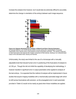
indicate the direction of flow forward (C) and in retrograde (F).](https://image.slidesharecdn.com/b9d15e8e-7423-429a-9418-53bc61f3c1fa-160106203545/85/Bulk_Alexander_Thesis-27-320.jpg)
![18
Pumping mechanics of the heart are not only critical to inducing adequate blood flow,
but also play an important role in heart morphology, as elastic stresses induced on
cardiomyocytes serve a mechanotransductive role in coordinating development [8]. It is
not fully understood how contraction in embryonic zebrafish cardiomyocytes compares
to adult cardiomyocytes, though it likely includes a similar process of binding between
the proteins, myosin and actin that comprise cytoskeletal filaments. In the adult human
heart, myocardial cell contraction initiates with an influx of extracellular calcium ions that
bind to troponin, which then activates the actin-myosin chain complex as illustrated in
Figure 2.5 [54]. This contraction induces an internal compressive stress within the
myocardial cell that is opposed by an intercellular tensile stress generated by the
connection to adjacent myocardial cells [55].](https://image.slidesharecdn.com/b9d15e8e-7423-429a-9418-53bc61f3c1fa-160106203545/85/Bulk_Alexander_Thesis-28-320.jpg)
![19
Figure 2.5: The Actin-Myosin Chain Complex
Diagram outlines the mechanism of muscle contraction through the actin-myosin chain cycle. Figure
taken from Cummings, 2001 [56].
The combination of these intercellular stresses between myocardial cells results in an
overall longitudinal and circumferential stress experienced by the heart during
contraction. The circumferential stress, also known as hoop stress, is linearly related to
the pressure within the chamber of the heart according to equation 2.1 below, where P
is the intramural pressure, σ is the hoop stress, R is the heart radius, and t is the
thickness of the myocardial, cardiac jelly, and endocardial layers [8].
𝜎 =
𝑅𝑃
𝑡
(2.1)
In addition to elastic stresses, stresses on the endothelial cells within the interior of the
heart generated by blood flow, or wall shear stresses, also play a critical role in heart
development. In order to calculate these wall shear stresses, assumptions have to be](https://image.slidesharecdn.com/b9d15e8e-7423-429a-9418-53bc61f3c1fa-160106203545/85/Bulk_Alexander_Thesis-29-320.jpg)
![20
made based on two non-dimensional parameters that characterize the flow conditions
within the heart. The first of these parameters is the Reynolds number, which describes
the ratio between inertial forces and viscous forces as shown in equation 2.2 below,
where D is diameter, U is the characteristic velocity, L is the characteristic length scale
and μ is viscosity [8]. If the Reynolds number is below 1000, the flow is said to be
laminar, and viscous forces dominate flow [8]. If the Reynolds number is greater than
approximately 3300, inertial forces dominate, and the flow is considered to be turbulent
[57].
𝑅𝑒 =
𝜌𝑈𝐿
𝜇
(2.2)
The second parameter is the Womersley number, which characterizes the stability of
the flow profile in pulsatile flow conditions, as is the case in the cardiovascular system.
The Womersley number is given in equation 2.3 below, where ω is the pulse frequency,
or heart rate [8]. If the Womersley number is below 1, the velocity profile will be
relatively parabolic, whereas if the Womersley number is greater than 1, the flow profile
will be irregular and unstable [58].
𝑊𝑜 = 𝐿√
𝜔𝜌
𝜇
(2.3)
Because the scale of the zebrafish embryonic heart is on the order of microns, the
Reynolds and Womersley numbers are low enough to be neglected, and all flow can be
considered to be laminar with a stable velocity profile [9, 59]. Therefore, terms in the
continuity and conservation-of-momentum equations that are proportional to these non-
dimensionalized characteristic parameters can be ignored.](https://image.slidesharecdn.com/b9d15e8e-7423-429a-9418-53bc61f3c1fa-160106203545/85/Bulk_Alexander_Thesis-30-320.jpg)
![21
In a Newtonian fluid, viscosity is defined as the ratio of shear stress to shear rate,
however adult human blood is considered to be a non-Newtonian fluid, as the viscosity
is non-constant, increasing with greater shear rate [60]. Blood viscosity is based on
both hematocrit count, or the percentage of blood consisting of RBCs, and fibrinogen
content, since fibrinogen (a secreted glycoprotein involved in clotting) binds together
RBCs [60]. In adult humans, the hematocrit count varies between 35-50%, but varies
between 10-15% in the embryo [8]. It is assumed that fibrinogen content is not greater
in the zebrafish embryo than the adult human, so based on the curves provided in
Figure 2.6, blood in the embryonic zebrafish can be estimated to be approximately
Newtonian and thus, of constant viscosity [60].
Figure 2.6: Shear Stress vs. Shear Rate of Blood at Various Hematocrit, Fibrinogen Levels
Viscosity is calculated from the slope of the shear stress-shear rate curve. Shear stress is linearly related
to shear rate in Newtonian fluids. Figure taken from Replogle et al., 1967 [60].](https://image.slidesharecdn.com/b9d15e8e-7423-429a-9418-53bc61f3c1fa-160106203545/85/Bulk_Alexander_Thesis-31-320.jpg)
![22
Since blood flow in the embryonic zebrafish heart is considered to be laminar,
Newtonian and having a stable velocity profile, wall shear stress in the embryonic heart
is derived from the simplified continuity equation and balance of momentum in a control
volume as shown in equation 2.4, where τw is wall shear stress, D is diameter, μ is
viscosity, Q is flowrate, vmax is the maximum velocity, and dP/dx is the pressure gradient
in the direction of flow [8, 61].
𝜏 𝑤 = −
32𝜇𝑄
𝜋𝐷3 = −
4𝜇𝑣 𝑚𝑎𝑥
𝐷
=
𝐷
4𝜇
𝑑𝑃
𝑑𝑥
(2.4)
By examining the first of these equations, it can be seen that as the diameter in the
heart decreases, the wall shear stress increases drastically, since downstream flowrate
is conserved. This observation is important since it predicts that at the constricted
regions within the heart such as the AVC, atrial inlet, and ventricular outlet, the wall
shear stress is dramatically greater than in the middle of the chambers [55]. This
difference in shear stress is important as it is likely involved in signaling that contributes
to the development of the endocardial “cushions” and later on, valves that form at the
constrictions as opposed to within the chambers.
Fluid vorticity is another parameter of the mechanical environment of intracardiac flow
that also likely plays an important contribution in heart development. Vorticity is defined
as local rotation within a fluid, and can be quantified by the curl of the velocity field.
Vorticity is understood to be vital for proper functionality in various biological systems,
such as in the adult aortic sinus, where a vortex structure aids in valve closure, in
preventing regurgitation, and regulating coronary flow [62, 63]. In the embryonic chick
and zebrafish, vortical flow patterns have been observed around the chamber](https://image.slidesharecdn.com/b9d15e8e-7423-429a-9418-53bc61f3c1fa-160106203545/85/Bulk_Alexander_Thesis-32-320.jpg)
![23
constrictions, and it has been hypothesized that these vorticities may be involved in
regulating developmental expansion of the chamber [9, 62, 64]. The presence of
vorticity causes a significant change in shear stress on the endocardium, therefore it
could operate as a key parameter in differentiation of signaling between various regions
of the interior heart [9].
2.4 Relationship of Mechanics to Heart Development
The vast majority of research addressing the role that intracardiac flow mechanics have
in regulating heart development has focused on methods to alter flow in order to
observe the heart’s developmental response. Because removal of blood from the
embryo could contribute to off-target effects impeding other non-cardiac physiological
regulators of development, the majority of experiments with wildtype embryos have
focused on altering the cardiac preload, or the pressure required to fill the atrium. In
chick embryos, two typical methods to reduce preload have consisted of either full or
partial ligation, or intentional closure, of either the chambers of the heart or the vitelline
veins preceding flow into the atrium [17, 65]. Full ligation of select vitelline veins has
resulted in a vast array of malformations later in development, including effects on the
ventricular septum, pharyngeal arch artery, and the semilunar and atrioventricular
valves [17, 66]. Partial ligation of the left atrium has resulted in irregular orientation of
myofibers as well as in dysfunction of the His-Purkinje System responsible for
coordinating contraction between cardiomyocytes [65, 67]. To increase cardiac loading,
partial ligation of the conotruncus just downstream of the chick embryo’s left ventricle is](https://image.slidesharecdn.com/b9d15e8e-7423-429a-9418-53bc61f3c1fa-160106203545/85/Bulk_Alexander_Thesis-33-320.jpg)
![24
used to force the heart to pump harder in order to eject through a smaller area [65].
Interestingly, conotruncal ligation results in dysfunction of the same systems as left-
atrial ligation, though with the complete opposite effect, such as equal but opposite
myofiber angle orientation [65, 67].
Because of the miniscule size of the zebrafish embryo, ligation is not possible as with
the chick embryo and therefore alternative methods are used to alter cardiac preload.
One method has consisted of the use of implanted glass beads inserted at the atrial
inlet and ventricular outlet in order to decrease and increase preload, respectively [9]. A
wide range of defects have been observed in zebrafish embryos as a result of this
method just as with the chick embryo, including blocked formation of the bulbus
arteriosus (a “third chamber” that functions as a capacitor), diminished cardiac looping,
abnormal valve formation, as well as notably impaired glomerular development [9, 68].
Perhaps the simplest method of altering flow in the zebrafish is achieved by altering the
heart rate. By simply decreasing or increasing incubation temperature below or above
the standard 28°C, heart rate can be decreased or increased, respectively, though this
also has significant effect on the overall rate of embryonic development [69, 70].
Tricaine methanesulfonate, the standard anesthetic for fish, can also be used to
decrease heart rate as well as induce hypertension, and the effects can be temporary
[71, 72]. Of all methods used to alter flow in the embryonic zebrafish heart, one of the
less-invasive methods that results in few off-target developmental defects is
centrifugation [50]. Centrifugation can be performed inside an incubator with the
embryos contained in embryo media-filled plastic tubes in order to maintain exposure to](https://image.slidesharecdn.com/b9d15e8e-7423-429a-9418-53bc61f3c1fa-160106203545/85/Bulk_Alexander_Thesis-34-320.jpg)
![25
the required osmotic environment [50]. Centrifugation can also be used to reduce the
cardiac preload at precise intervals in order to study the time-dependent role of flow
mechanics in cardiac development [50].
It is expected that the primary cause of these morphological impairments resulting from
altered loading is due to changes in the characteristic cyclical shear stress experienced
by the endothelial cells. Mechanical stress on an endothelial cell, whether due to elastic
tension or compression or shear stress, is known to alter the cytoskeletal structure of
the cell as well as the configuration of ion channels, caveolae, pumps and various other
receptors on the apical membrane [73, 74]. These changes in configuration result in
changes to intracellular signaling cascades that regulate gene expression [74].
Additionally, shear stress has been shown to alter the arrangement and organization of
endothelial cells in culture (Figure 2.7), which has significant effects on intercellular
signaling that can also contribute to gene expression [73, 75].](https://image.slidesharecdn.com/b9d15e8e-7423-429a-9418-53bc61f3c1fa-160106203545/85/Bulk_Alexander_Thesis-35-320.jpg)
![26
Figure 2.7: Effect of Flow-Induced Shear Stress on Cultured Endothelial Cells
Left: Endothelial cells cultured under static conditions. Right: Endothelia cultured under 24 hours of
steady, laminar flow at 7.5 μmHg pressure. Image taken from Topper and Gimbrone, 1999 [73].
Several mechanisms are responsible for signal transduction on the membrane surface
of endothelial cells. Certain potassium ion channels have been shown to require elastic
stretch of the membrane in order to open, and shear stress is necessary to expose
calcium ion channels by essentially pushing them open via the movement of adjoined
membranous cilia [36, 76]. One of the more important transducers of shear stress is the
extracellular protein framework of the glycocalyx [77]. When shear stress acts on the
glycocalyx, it produces a torque, which causes deformation of the underlying hexagonal
lattice-structured, actin cortical web (ACW) [77]. Deformation of the ACW is necessary
for the formation and opening of caveolae, large membranous invaginations responsible
for an array of signaling functions [77]. The presence of shear stress during endothelial
differentiation has been shown to be necessary for the formation of this actin web as
well [78].](https://image.slidesharecdn.com/b9d15e8e-7423-429a-9418-53bc61f3c1fa-160106203545/85/Bulk_Alexander_Thesis-36-320.jpg)
![27
Though multiple endothelial extracellular mechanotransducers have been discovered, in
many cases the signaling pathways that they activate to modulate downstream gene
expression have not been revealed, or still require the discovery of various kinases,
receptors, or genes to “fill the gaps.” One well-understood pathway involves the
activation of extracellular signal-regulated kinase ½, or ERK ½, through cascades
originating with Tyrosine kinase and G-protein coupled receptors on the apical
membrane (Figure 2.7) [79]. ERK ½ is known to mediate phosphorylation of key
transcription factors, as well as stimulate sustained production of nitric oxide [79, 80].
Figure 2.8: Model of Shear Stress-Mediated Mechanotransduction in Endothelial Cells
Model of receptors and signaling cascades involved in activation of ERK ½ in response to shear stress.
Figure taken from Traub and Berk, 1998 [80].](https://image.slidesharecdn.com/b9d15e8e-7423-429a-9418-53bc61f3c1fa-160106203545/85/Bulk_Alexander_Thesis-37-320.jpg)
![28
Despite the fact that most stress-mediated signaling pathways controlling gene
expression have yet to be discovered, several key genes in the embryonic heart have
been determined to be flow and/or stress-responsive. Three of the most studied of
these genes have been GATA-binding protein 4 (GATA4), Filamin-C (FLNC), and
Kruppel-like Factor 2 (KLF-2) [79, 81, 82]. GATA4 is a heart development-regulating
transcription factor that has been shown to be necessary for mediation of cardiac
remodeling in response to changes in cardiac loading, as expression has been shown
to be highly responsive to ventricular swelling [79]. Along with the gene SMAD4,
GATA4 has also been shown to be involved in regulating septum and atrioventricular
valve formation [79, 83]. Filamin C is a cytoskeletal protein that controls the alignment
of myocardial cells and formation of myofibrils at myotendinous junctions in order to
maintain structural integrity of the myocardium and thus, efficiency of contractility [81,
84]. Mutations in FLNC have been shown to cause a thickening of the myocardial
tissue, resulting in hypertrophic cardiomyopathy, though it is still unclear whether these
mutations would be induced by altered flow [85]. Finally, KLF-2, a transcription factor
which is expressed strongly in regions of high shear, is necessary for formation of an
atrioventricular valve and for erythropoiesis, or RBC generation [36, 82, 86-88]. By
knocking down KLF-2, an abnormal decrease in the size of the vessels occurs, which
results in severe hemorrhaging throughout the cardiovascular system [36]. Though
various important phenotypes have been found to be highly correlated with the
expression of these genes, it is expected that these phenotypes are linked to the
expression of a network of pathways combining other key developmental genes as well.](https://image.slidesharecdn.com/b9d15e8e-7423-429a-9418-53bc61f3c1fa-160106203545/85/Bulk_Alexander_Thesis-38-320.jpg)
![29
It is probable that any mutation that affects embryonic cardiac morphology will affect
flow, so the response of aspects of flow involved in mechanotransduction to changes in
many developmentally-related genes must also be understood. A few other important
genes associated with heart development are c-Myc, EGFR, ET-1, NOS-3, and HERG
[82, 86, 89-91]. C-Myc is necessary for the proliferation of cardiomyocytes, and is also
likely involved in signaling of later key cardiogenesis-related genes [89]. EGFR is
another precursor gene necessary to develop receptors needed for ERK ½ signaling,
and inhibition of EGFR causes severe chamber dilation with greater narrowing of the
constrictions at the AVC and ventricular outlet [79, 80, 90]. ET-1 and NOS-3 are both
important shear-responsive genes similar to KLF-2, though whereas NOS-3 and KLF-2
are expressed in response to high shear stress, ET-1 is expressed in response to low
shear [82, 86]. Knockdown of NOS-3 results in impaired endothelial nitric oxide
reception and septal defects, and knockdown of ET-1 results in similar defects to
vitelline vein ligation in chick embryos [36]. HERG, or the human homologue gene in
the zebrafish, ZERG, is necessary for coordinating contraction between the atrium and
ventricle [91]. Mutations in ZERG cause prolonged chamber relaxation in addition to
arrhythmia between contractions of the atrium and ventricle, indicating that ZERG is
necessary for the activation of a conductive ion channel between the chambers in the
zebrafish [91].
Of particular importance to this research are the genes involved in valve development at
the AVC. In addition to KLF-2, Hyaluronic Synthase 2 (HAS2), the “Cardiofunk gene”
(CFK), and Notch-1b are all necessary for the formation of the endocardial cushions](https://image.slidesharecdn.com/b9d15e8e-7423-429a-9418-53bc61f3c1fa-160106203545/85/Bulk_Alexander_Thesis-39-320.jpg)
![30
preceding valvulogenesis at the AVC [87, 92-94]. MicroRNA-23 is important in
endocardial cushion formation as well, as it is needed to limit the expression of HAS2,
which induces unlimited endocardial cushion growth in the absence of microRNA-23
[92]. Vermot et al. tested the expression of three genes known to be involved in valve
development in response to changes in flow in embryonic zebrafish and discovered a
transcription factor of the KLF family, KLF2a, was responsive to retrograde flow in the
AVC [87]. GATA1 and GATA2 morphants were used to manipulate the blood viscosity
by reducing the hematocrit count in order to alter the wall shear stress [87]. What was
discovered was that induced consistent forward flow would result in a malformed
atrioventricular valve, however wildtype embryos with a normal period of retrograde flow
that would produce the same theoretical magnitude of shear stress would develop
normally [87]. The absence or existence of reverse flow did not solely dictate normal
valvulogenesis, though [87]. Instead, a combination of an acceptable range in
magnitude and cyclical direction of shear stress are needed for normal differentiation of
the endocardial cushions [87]. Not only did KLF2a become misexpressed under the
absence of normal retrograde flow conditions, but by knocking out KLF2a, the same
valve malformations occurred, making KLF2a an important link between retrograde flow
and valvulogenesis [87].](https://image.slidesharecdn.com/b9d15e8e-7423-429a-9418-53bc61f3c1fa-160106203545/85/Bulk_Alexander_Thesis-40-320.jpg)
![31
Figure 2.9: Relationship Between Retrograde Flow, KLF2a, and Valvulogenesis
A: As the embryo develops from 36 hpf to 58 hpf, KLF2a expression (darkened regions) becomes
localized and condenses at the AVC (pink box, white arrow) and ventricular outlet (black arrow). B-C:
Endothelial cells at the AVC in controls (WT), GATA2 MOs (low shear stress, reduced retrograde flow),
and KLF2a MOs at 72 hpf. GATA2 and KLF2a MOs lack sufficient endocardial cushions for valve
formation. D: Summary diagram of KLF2a function. Figure taken from Vermot, et al., 2009 [87].
Calculations of shear stress made by Vermot et al. were limited in accuracy because
they failed to address the dynamic change in diameter of the AVC, only using an
average estimated diameter in equation 2.4 [87]. Though retrograde flow was identified
as necessary for KLF2a expression, the shear stresses associated with this flow
necessary to induce expression remain unknown. Since retrograde flow only occurs
during a specific period of the cardiac cycle, particular pumping mechanics conditions
must be present to induce such a flow characteristic. Aim 1 of this thesis is focused on
these mechanical influences driving the occurrence of retrograde flow through the AVC.](https://image.slidesharecdn.com/b9d15e8e-7423-429a-9418-53bc61f3c1fa-160106203545/85/Bulk_Alexander_Thesis-41-320.jpg)
![32
2.5 Methods for Analyzing Embryonic Heart Function
In order to quantify intracardiac flow parameters within the embryonic heart, imaging
techniques must have the capacity to acquire the spatial and temporal resolution
necessary to perform various computational flow-measurement methods. Due to the
microscopic scale of the embryonic heart, standard medical imaging modalities such as
ultrasound, MRI, and CT cannot attain such a scale of resolution [55]. One method
used in chick embryos is optical coherence tomography (OCT), which consists of the
emission of laser light and subsequent absorption of the reflected laser to develop a 2D
image [16, 55]. OCT has a penetration depth of up to 2 mm and a resolution of
approximately 10 μm, which is not ideal for measurements in the embryonic zebrafish,
though is excellent for the chick embryo heart [16, 18, 95]. This low spatial resolution
has prompted the development of cross-correlation algorithms that perform 3D-image
restructuring of the embryonic heart in order to create finite element models which are
then used to determine the elastic properties of the myocardial tissue [18, 95]. After the
development of a laser gating method by Jenkins et al. in 2006, OCT images were able
to be captured at a rate fast enough to perform microscopic particle image velocimetry
(PIV) using red blood cells as tracer particles [96-98]. OCT has been used to study the
velocity profile and strain rates at the ventricular outlet in the chick embryo heart, though
the accuracy of this method is hindered by the imaging angle [16, 18, 95]. Velocity
measurements can encounter significant noise if prone to interference from the heart
wall, and blood cell velocities perpendicular to the OCT laser often go unmeasured [16].](https://image.slidesharecdn.com/b9d15e8e-7423-429a-9418-53bc61f3c1fa-160106203545/85/Bulk_Alexander_Thesis-42-320.jpg)
![33
Two other imaging modalities used to analyze embryonic heart function are confocal
and bright-field microscopy. Confocal microscopy requires the use of fluorescence
labeling to view internal features of a semi-transparent specimen by exciting
fluorophores [41]. The focal plane thickness of confocal microscopy is very low, so it
has been used to generate accurate 3-D reconstructions of the embryonic zebrafish
heart [41, 45, 99]. Unfortunately, confocal microscopy lacks the temporal resolution
necessary to analyze the intracardiac flow environment of the embryonic heart [41].
Bright-field microscopy on the other hand, does have that capability. Bright-field
microscopy is the simplest imaging modality, though it requires the use of a transparent
sample, so spatial resolution is simply dictated by the lighting intensity [55]. Fortunately,
zebrafish embryos are transparent, making this imaging modality one of the most
widely-used in embryonic zebrafish research. The focal plane thickness of bright-field
microscopy is much greater than that of confocal microscopy, rendering it an
inadequate method for 3-D image reconstruction; however unlike confocal microscopy,
the temporal resolution is more than adequate for acquiring computational flow
measurements of the intracardiac flow. Because of these advantages, experiments
performed as part of the research comprising this thesis utilized bright-field microscopy.](https://image.slidesharecdn.com/b9d15e8e-7423-429a-9418-53bc61f3c1fa-160106203545/85/Bulk_Alexander_Thesis-43-320.jpg)
![34
Figure 2.10: Embryonic Zebrafish Heart Imaged Under OCT (1), Confocal (2), and Bright-Field
Microscopy (3)
1: Ventral-Cranial view of the zebrafish embryo under Optical Coherence Tomography at 72 hpf (top) and
120 hpf (bottom). Bright regions are created by blood flow and the white arrow points out the location of
the heart. Image taken from Kagemann, et al., 2008 [100]. 2: Embryonic heart under confocal microscopy
at two cardiac cycle time points imaged at 108 hpf. “a” is the atrium, “v” is the ventricle, and “av” is the
AVC. Image taken from Hove, et al., 2003 [9]. 3. Embryonic heart under bright-field microscopy at two
cardiac cycle time points imaged at 48 hpf. “A” is the atrium and “V” is the ventricle. Image taken using
Olympus SZX12 bright-field stereomicroscope.
Particle Image Velocimetry (PIV) is a computational flow-measurement method that
generates a velocity vector field from either 2D or 3D image sequences of a fluid
consisting of tracer particles of an intensity contrasting that of the background. In
experimental flow loops such as those used for studying turbulence, tracer particles are
typically seeded into the fluid and intensity contrast is generated via illumination by a
laser sheet [101]. When imaging the embryonic hearts of chicks and zebrafish
however, red blood cells are used as tracer particles [101, 102]. Each frame of an
image sequence of a fluid is divided into a grid, and a cross-correlation algorithm is](https://image.slidesharecdn.com/b9d15e8e-7423-429a-9418-53bc61f3c1fa-160106203545/85/Bulk_Alexander_Thesis-44-320.jpg)
![35
used to find the displacement of grid segments of similar particle orientation [103]. A
velocity vector is then generated for each grid segment by dividing the time between
frames by the grid segment displacement [103]. Velocities in between these grid
segments are able to be calculated through interpolation, making PIV an excellent
method for analyzing velocity profile. Methods utilizing PIV have been developed to
calculate further parameters such as pressure, wall shear stress, and vorticity [9, 104,
105].
Because bright-field microscopy can be used to generate such high-resolution images
of the embryonic zebrafish heart (Figure 2.10), it would seem that the intensity contrast
of the individual red blood cells would make PIV an optimal method to analyze the flow
mechanics. However, the scale of the red blood cells compared to the overall size of
the heart is significantly large at the developmental stages analyzed in this thesis, thus
the number of tracer particles in the overall fluid domain is relatively low. This is not
ideal for PIV, as more accurate results are able to be attained with a greater number of
smaller particles [106]. The size of the RBCs also affects how close they flow to the
wall, so flows adjacent to the endocardium that only consist of plasma go undetected
[106]. Because PIV measures velocity vectors by finding correlating pixel arrangements
within grid segments, deformation in the RBCs caused by pressure changes can
prevent the software from recognizing the RBC displacement, causing further error.
Endothelial cells are also of the same size as red blood cells, so PIV software
recognizes the walls of the heart as moving particles within the fluid [106]. When the
endothelial cells move in the opposite direction of the RBCs, vortices are calculated](https://image.slidesharecdn.com/b9d15e8e-7423-429a-9418-53bc61f3c1fa-160106203545/85/Bulk_Alexander_Thesis-45-320.jpg)
![36
along the heart walls which severely disrupt intracardiac velocity calculations [55].
These limitations have not completely rendered PIV as an ineffective tool for analyzing
intracardiac flows, but they have forced accurate analysis to be confined to only large-
scale flow regions within the chambers [9, 104, 105].
Because PIV is such a powerful tool for visualizing the intracardiac flow environment,
several attempts have been made to remove the heart walls from velocity calculations.
The first attempt was through the development of a manual mask-drawing algorithm to
eliminate the background signal, though PIV software would often still incorporate the
dynamic background mask into velocity calculations [55]. A second method developed
was to incorporate fluorescence labeling of red blood cells so that PIV software could be
manipulated to only recognize fluorescent pixels [71, 107, 108]. Unfortunately, the
fluorescence signal was unable to be captured accurately when imaging at the high
frame rates needed to perform PIV calculations [107]. Lastly, the most promising
method developed by Jamison et al. consists of the use of cardiac phase filtering to
remove patterns that repeat over multiple cardiac cycles, leaving only the RBCs in the
image [108]. Pixel patterns often do not correlate with that of subsequent cardiac cycles
however because cardiomyocytes do not move in the exact same motion with each
heartbeat, because heart rate often exhibits slight fluctuations over time, and because
microscopes are often subject to some vibration [108]. This method is therefore still
prone to significant error, though due to the prominence of ongoing research on the role
of intracardiac flow mechanics in heart development, it is likely that a highly accurate
method of PIV will be developed in the near future.](https://image.slidesharecdn.com/b9d15e8e-7423-429a-9418-53bc61f3c1fa-160106203545/85/Bulk_Alexander_Thesis-46-320.jpg)
![37
The flow-measurement method used for the research composing this thesis was
inspired by an imaging modality referred to as ‘laser scanning microscopy’ (LSM).
Rather than capture 2-D image sequences of an internal region of interest within the
heart, LSM consists of the rapid reflection and absorption of a single laser linescan in
one dimension [71]. The result is a spatiotemporal (ST) plot, or a kymograph,
consisting of pixel data generated from the laser displayed along the vertical axis with
respect to its change in time along the horizontal axis [71]. Laser scans can be
captured as fast as 2,050 lines per second, making this method ideal for measuring
blood cell velocity [71]. When the laser is directed parallel to the blood flow, red blood
cells flowing along the beam produce streaks in the resultant spatiotemporal plot with an
angle corresponding to the blood cell’s velocity [71]. By combining this spatiotemporal
velocity data with dynamic diameter-change data collected by orienting the laser
perpendicular to the flow direction, accurate calculations of flowrate, stroke volume, and
cardiac output have been made in the zebrafish dorsal aorta [71].
Though successful in the dorsal aorta, it is far more difficult to orient an LSM laser in-
line with blood flow within the much less uniformly-shaped heart, especially at a region
of selected interest [71]. Fortunately, because of the excellent spatial resolution of
bright-field microscopy, the quantitative method of spatiotemporal analysis used for
LSM scans has been applied to image sequences captured with a bright-field
microscope. This allows for one-dimensional regions of interest, or “reference lines” to
be manually selected from 2-D image sequences of the heart in order to generate ST
plots. Computational software that utilizes spatiotemporal analysis of bright-field-](https://image.slidesharecdn.com/b9d15e8e-7423-429a-9418-53bc61f3c1fa-160106203545/85/Bulk_Alexander_Thesis-47-320.jpg)
![38
acquired, high-speed image sequences of the embryonic zebrafish heart was developed
in 2013 by Johnson, et al., called the “Kymograph Analyzation Tool,” or KAT [109]. Due
to the access to bright-field microscopy, KAT was determined to be the most accurate
flow-measurement method available for measuring intracardiac flow as part of this
research.
After image sequences of the embryonic heart are uploaded into KAT, they must
undergo several preprocessing steps in order to enhance the accuracy of analysis.
First, any vibration that may have caused shake in the image sequence is removed by
shifting each frame such that the intensity of pixels in a static, manually-selected region
align to the pixels of that region in the first frame. Fluctuations in lighting intensity could
also severely affect velocity calculations, so intensity is then normalized across the
image sequence using another manually-selected static region. This is done by
calculating the average intensity of the pixels in that region so that all pixels in the rest
of the image sequence are multiplied by a factor such that the pixels within that region
retain the same average intensity [109]. Finally, since calculated parameters are
averaged across cardiac cycles, the number of frames per cycle, or the heart rate, is
calculated in order to generate a separate ST plot for each cycle. To do this, a
reference line is selected over any region overlapping the heart. The variance between
the pixels on the line in the first frame and each subsequent frame is then calculated
and the frame with the least variance is determined [55]. The number of frames
between the frame with least variance to the first is divided from the frame rate of the
high-speed camera to determine the heart rate [55].](https://image.slidesharecdn.com/b9d15e8e-7423-429a-9418-53bc61f3c1fa-160106203545/85/Bulk_Alexander_Thesis-48-320.jpg)
![39
After preprocessing, spatiotemporal analysis of flow parameters begins with calculation
of the lumen diameter by positioning a reference line perpendicular to the flow. Though
the atrial inlet remains approximately static relative to the rest of the heart, most other
regions of the heart exhibit considerable movement throughout each cardiac cycle.
Because it is typically necessary to analyze regions other than the inlet, a feature of the
KAT software allows for the location of the reference line to migrate with the movement
of the heart throughout the cardiac cycle through the selection of “key frames” so that
the position of the reference line between each key frame is interpolated. On the
resultant ST plot, lumen diameter is then measured simply by manual selection of points
along the inner edge of the endocardium as shown in Figure 2.11 [109].](https://image.slidesharecdn.com/b9d15e8e-7423-429a-9418-53bc61f3c1fa-160106203545/85/Bulk_Alexander_Thesis-49-320.jpg)
![40
Figure 2.11: Example Spatiotemporal Plots of Diameter and Velocity Generated with KAT
Top: Location of reference line (left) and resultant spatiotemporal plot (right) to calculate lumen diameter
at the atrial inlet of a 48 hpf WT zebrafish embryo. Manually-selected points on the endocardial edge are
indicated in green. Bottom: Location of reference line (left) and resultant spatiotemporal plots (right) to
calculate velocity from the streak angle. The sliding average of the pixel intensity was subtracted in the
processed spatiotemporal plot. The white square in the processed plot indicates a bin undergoing radon
transform.
To calculate velocity, a reference line is oriented parallel to the flow at the center of the
flow profile to produce the unprocessed, streaked ST plot shown in Figure 2.11. In
order to strengthen the signal-to-noise ratio of the streak angles corresponding to the
RBC velocities, the sliding average of the pixel intensity of the image sequence is
subtracted from the pixel intensity of each frame [109]. Therefore, all static portions of
the image sequence are removed so that only the heart appears over a black
background, resulting in the processed ST plot in Figure 2.11. Velocity measurements
are made at 100 evenly-spaced time points along the cardiac cycle by measuring the
streak angle across “bins” of 21-frame-width about each point. To calculate the streak
angle, radon transforms were performed on each bin as illustrated in an example bin](https://image.slidesharecdn.com/b9d15e8e-7423-429a-9418-53bc61f3c1fa-160106203545/85/Bulk_Alexander_Thesis-50-320.jpg)
![41
shown in Figure 2.12 [109]. A radon transform is generated by projecting lines across
the bin at angles ranging from 0° to 180° that generate a plot of the bin pixels along the
projected line on the vertical axis versus the angle of projection along the horizontal axis
(Figure 2.12) [109]. The variance is then calculated from the derivative of the radon
transform, or more specifically, the pixel intensities along the line at each angle, and the
angle with the greatest variance is used as the velocity streak angle [109]. A bin length
of 21 was determined to result in minimum error when calculating the variance of these
radon transforms [109].](https://image.slidesharecdn.com/b9d15e8e-7423-429a-9418-53bc61f3c1fa-160106203545/85/Bulk_Alexander_Thesis-51-320.jpg)
![42
Figure 2.12: Velocity Calculation of an Example ST Plot Bin via Radon Transform
A: Orientation of example radon transform at projection angles of 0°, 90°, and 138°. B: The projected line
at each angle ranging from 0° to 180° produces the radon transform plot shown. C: Plot of the variance
of the derivative of the radon transform plot in (B) at each projection angle. A projection angle of 138°
induces maximum variance, therefore the velocity of this bin is v=tan(138°-90°)=1.11 pixels/frame. Figure
taken from Johnson, et al., 2013 [109].
The set of 100 velocity measurements calculated across each cardiac cycle is averaged
with the velocities of the subsequent cardiac cycles, and velocities outside of a variance
threshold are then eliminated to remove noise [109]. By performing several velocity
measurements across the velocity profile of the atrial inlet in several 48 hpf WTs, it was
determined that the average velocity of the profile was equal to 74% of the center
velocity [55]. The flow rate at each of the 100 time points is estimated by taking the](https://image.slidesharecdn.com/b9d15e8e-7423-429a-9418-53bc61f3c1fa-160106203545/85/Bulk_Alexander_Thesis-52-320.jpg)
![43
product of the average velocity and the lumen area, assuming that the area is a circular
profile of the calculated lumen diameter, as shown in equation 2.5 where Q(t) is
flowrate, v(t) is velocity, and D(t) is diameter [109]:
𝑄(𝑡) = 0.74
𝜋
4
𝑣(𝑡)𝐷(𝑡)2
(2.5)
Accumulated Volume is then calculated at each 100th
of the cycle through the sum of
the previous differential volumes, which are calculated by the product of the time
corresponding to 1/100th
of the cycle (Δt) and the instantaneous flow rate, Q(t) as shown
in equation 2.6, where Vac is the accumulated volume [109]:
𝑉𝑎𝑐(𝑡) = ∑ 𝑄(𝑡)𝑖∆𝑡𝑖=𝑡
𝑖=0 (2.6)
The accumulated volume at the end of the cardiac cycle corresponds to the stroke
volume of the heart, and the cardiac output is equal to the product of the stroke volume
and heart rate [109]. The retrograde flow fraction (RF), or the fraction of the volume of
blood moving in reverse across the measured region of interest, is calculated as shown
in equation 2.7 by taking the ratio of the sum of the negative differential volumes over
the sum of the positive differential volumes [109]:
𝑅𝐹 =
‖∑ 𝑄(𝑡) 𝑖∆𝑡 < 0‖
∑ 𝑄(𝑡) 𝑖∆𝑡 > 0
(2.7)
Because blood is pushed ahead of the contractile wave in the embryonic zebrafish heart
tube and atrium prior to valve formation, the instantaneous heart volume cannot
accurately be used to predict stroke volume [45, 109]. Therefore, previous methods to
calculate stroke volume and cardiac output, which measured the difference in end-
diastolic and end-systolic volumes (EDV, ESV), would result in considerable
underestimation in comparison to this method [109]. Spatiotemporal analysis with KAT
is an exceedingly accurate method of measurement with respect to diameter and](https://image.slidesharecdn.com/b9d15e8e-7423-429a-9418-53bc61f3c1fa-160106203545/85/Bulk_Alexander_Thesis-53-320.jpg)
![44
velocity calculations. The error in diameter measurement is ±1 pixel, so with a
resolution ranging between 1024 - 1310 pixels/mm of the bright-field microscope used
for the research in this thesis, the error in diameter ranges as low as ±0.76 - ±0.98 μm
[109]. Error in streak angle is ±1.5°, so with frame rates used in this research ranging
between 1000 - 1500 frames/s, the error in velocity ranges between ±0.020 - ±0.038
mm/s [109].
Despite the advantages that spatiotemporal analysis holds in analyzing embryonic
zebrafish intracardiac flow, several limitations inhibit its accuracy in quantifying flow
rates and overall heart function parameters. The first and most obvious limitation lies in
the assumption that the lumen area is of a circular profile, which drastically affects the
accuracy of flowrate calculations [109]. Since an imaging modality that can accurately
measure intracardiac flow in the embryonic zebrafish in three dimensions has yet to be
developed, the circular-profile assumption has been used in the majority of previous
research consisting of the measurement of similar parameters [9, 110]. Another
prominent limitation arises from the assumption that mean velocity is equal to 74% of
the centerline velocity. Because the velocity ratio of 0.74 was determined via multiple
velocity measurements across a profile of the heart, and because velocities near the
endocardial wall are unmeasurable due to a lack of RBC flow near the wall, the mean
velocity may be underestimated. Also, since this velocity ratio was calculated at the
atrial inlet in just a few wildtype zebrafish, this ratio could potentially not hold in other
regions of the heart or in experimentally-treated embryos [109]. The purpose of Aim 2
of this thesis was to develop methodology to address these limitations by analyzing](https://image.slidesharecdn.com/b9d15e8e-7423-429a-9418-53bc61f3c1fa-160106203545/85/Bulk_Alexander_Thesis-54-320.jpg)

![46
3. AIM 1
Since it has been illustrated that retrograde flow at the atrioventricular canal (AVC) in
the post-tube/pre-valve embryonic heart is necessary for valvulogenesis [87], the
purpose of aim 1 was to investigate the pumping mechanics influencing the induction of
this retrograde flow. By non-invasively altering the cardiac preload in an experimental
group of embryos, retrograde flow was able to be inhibited such that pumping
mechanics could be compared with a control group of wildtype (WT) embryos exhibiting
normal retrograde flow. Image sequences of the embryonic zebrafish heart were
computationally analyzed using spatiotemporal analysis at both 48 and 55 hours post-
fertilization (hpf), two key developmental time points in which the retrograde flow
required for normal valve formation is prevalent [87]. Descriptive parameters of the
pumping mechanics were then statistically compared between groups to determine
those necessary for the presence of retrograde flow. Threshold ranges of two
parameters: pressure associated with expansion and contraction of the atrium and
ventricle, and resistance due to contractile closure of the atrium and AVC were
determined to be mechanistically associated with the presence of retrograde flow.
3.1 Methods: Experimental Groups
Retrograde flow through the AVC begins at the onset of cardiac looping and continues
until the formation of a valve around 105-111 hpf [34, 40, 41, 43]. During looping,
retrograde flow is less prominent, so the analysis time point of 48 hpf was chosen](https://image.slidesharecdn.com/b9d15e8e-7423-429a-9418-53bc61f3c1fa-160106203545/85/Bulk_Alexander_Thesis-56-320.jpg)
![47
because it marks the end of cardiac looping, when the fraction of flow moving in
retrograde becomes much more significant and occurs for a greater duration of the
cardiac cycle [30, 34]. Though the retrograde flow involved in valve formation maintains
prominence beyond 55 hpf, the second analysis time point of 55 hpf was chosen
because it marks the beginning of obstruction of the heart under bright-field microscopy
caused by the onset of pigmentation [22, 23]. These time points were also chosen for
analysis to enable comparison with previous studies [40, 50, 87, 111].
After centrifugation was used to alter the cardiac preload in an experimental group of
embryos, embryos with consistent retrograde flow were qualitatively separated from
those without. Centrifugation has been shown to cause increase in variation in multiple
flow parameters depending on the range of development time points that centrifugation
is performed across [50]. Therefore, only embryos without noticeable morphological
defects other than the absence of retrograde flow were used in the experimental group
(N=17). Of the control group of wildtype embryos, approximately 5% either exhibited an
absence of retrograde flow or did not experience retrograde flow to the extent of the
other wildtypes. Because this study is only concerned with the influence of pumping
mechanics on the presence of retrograde flow, rather than incidence of retrograde flow
absence, these embryos were not included in the control group (N=20), and instead
included in the experimental group. Thus, of the experimental group of embryos not
experiencing retrograde flow, 8 were wildtype embryos exhibiting a sporadic phenotype,
and 9 were centrifuged embryos.](https://image.slidesharecdn.com/b9d15e8e-7423-429a-9418-53bc61f3c1fa-160106203545/85/Bulk_Alexander_Thesis-57-320.jpg)
![48
3.2 Methods: Zebrafish Breeding and Embryo Preparation
Wildtype zebrafish (Danio rerio) were raised and bred in accordance with Westerfield
[112] at a zebrafish handling facility located on the main campus of Colorado State
University. Though these fish are considered to be wildtype, inbreeding has occurred
for many generations. Fate-mapping experiments have been performed to determine
the effect of zebrafish inbreeding in comparison to wild isolates, however it is unclear
whether or not they have displayed any genetic variation that would affect the outcome
of studies related to cardiac development [113]. In fact, the use of inbred strains is
advantageous in that by reducing genetic variability of the parent fish, random variability
in embryonic development of the offspring is minimized so that experimental outliers
can be avoided [55].
Lighting in the zebrafish handling facility is automated to coordinate with the fish’s
circadian rhythm, therefore matings were set up prior to when lights turn on at 7:00 am,
the time at which the fish are most susceptible to breed. To prepare for breeding,
parent zebrafish were placed in breeding tanks the night prior with a transparent barrier
used to separate the males and females overnight. In order to increase the probability
of yielding a large number of eggs, two females were placed in each tank opposite one
male. The barrier was removed to initiate breeding, and a sieve at the bottom of the
breeding tank allowed the fertilized eggs to fall through, preventing from being
consumed by the parent fish. Eggs were then collected after one hour of breeding to](https://image.slidesharecdn.com/b9d15e8e-7423-429a-9418-53bc61f3c1fa-160106203545/85/Bulk_Alexander_Thesis-58-320.jpg)
![49
limit the error in developmental stage determination to the timed age ± 30 minutes post-
fertilization.
After eggs were collected, they were stored in petri-dishes of E3 media, or embryo
water, in an incubator at the standard temperature of 28°C [112]. Embryos removed
from their chorion, or egg sac, require additional calcium for survival, so E3 media is
used to provide this needed calcium, as well as solutions of various other nutrients to
optimize the embryos’ nutritional exposure [112]. A stock solution of 0.5 g/L of
methylene blue trihydrate (Acros Organics) was diluted into the E3 media just after
collection to act as an antimicrobial agent and prevent the invasion of paramecium.
Embryo media was also replaced daily to ensure the prevention of mold growth inside
the petri dish. Since some experimental embryos began centrifugation regimes at 24
hpf (± 0.5 hpf), all embryos were dechorionated (Figure 3.1) just prior to this time using
tweezers and forceps by carefully peeling off the chorion in order to easily position the
embryos at optimal viewing angles during imaging.](https://image.slidesharecdn.com/b9d15e8e-7423-429a-9418-53bc61f3c1fa-160106203545/85/Bulk_Alexander_Thesis-59-320.jpg)
![50
Figure 3.1: Scale of Chorionated and Dechorionated Zebrafish Embryos
Embryos at 55 hours post-fertilization (hpf) with and without a surrounding chorion are shown next to a
U.S. penny for scale. Image taken from Johnson, et al., 2013 [109], 2015 [50].
3.3 Methods: Centrifugation
Since alternative methods to alter cardiac preload are invasive and/or result in various
irreversible off-target developmental defects that would be detrimental to the
experimental methodology of this study, centrifugation was chosen as the optimal option
to alter the biomechanical environment in timed increments [9, 68-72]. Centrifugation
causes a decrease in cardiac preload by effectively removing the amount of blood that
returns to the heart by inducing “pooling” of the blood to the embryo’s extremities [55].
Embryos were centrifuged during one of four six-hour increments determined by key
developmental stages defined by Kimmel as shown in Table 3.1 [30, 50]. Centrifuging
at these different stages was determined by Johnson, et al. to have a significantly
different and more variable effect on heart morphology and function depending on the](https://image.slidesharecdn.com/b9d15e8e-7423-429a-9418-53bc61f3c1fa-160106203545/85/Bulk_Alexander_Thesis-60-320.jpg)
![51
period of induced centrifugation [50]. By centrifuging at earlier stages (24-36 hpf),
longer-lasting changes in heart morphology and function result, whereas centrifuging at
later stages (36-48 hpf) results in temporary alterations from which embryos often
recover by 55 hpf [50]. The effect of centrifugation on retrograde flow has not been
studied at the AVC, though it has been studied at the atrial inlet. In Johnson’s study,
regardless of the period of centrifugation used, a group of embryos will experience an
increase in the variance of observed retrograde flow fraction (RF) at the atrial inlet,
rather than an overall increase or decrease in RF [50]. Therefore, in the current study,
all four increments of centrifugation were further evaluated and only embryos exhibiting
an absence of observable retrograde flow at the AVC were selected for analysis as part
of the experimentally ‘affected’ group. Though it was visibly apparent based on the
number of red blood cells (RBCs) flowing across the AVC that these experimental
embryos lacked retrograde flow, it is highly probable however that there still remains a
small amount of plasma flowing in reverse each cardiac cycle. The number of embryos
centrifuged during each developmental stage is shown in Table 3.1:
Table 3.1: Periods of Centrifugation and Associated Developmental Stages
Group # Time Period Developmental Stage Amount
1 24 hpf 30 hpf Onset of Circulation 3
2 30 hpf 36 hpf Early Cardiac Looping 3
3 36 hpf 42 hpf Mid-Cardiac Looping 2
4 42 hpf 48 hpf Late Cardiac Looping 1
To load embryos into the centrifuge, they were first inserted into small pieces of polymer
tubing (Cole-Parmer, FEP tubing) of 1/32” inner diameter by attaching the tubing to the](https://image.slidesharecdn.com/b9d15e8e-7423-429a-9418-53bc61f3c1fa-160106203545/85/Bulk_Alexander_Thesis-61-320.jpg)

![53
Figure 3.2: Centrifugation Experimental Setup
A: Embryos were inserted into plastic polymer FEP tubing of 1/32” inner diameter via pipette to constrain
the embryo. B: Plastic polymer tubes were then inserted into a larger centrifuge tube partially-filled with
low-melting agarose gel to prevent the embryo from sliding out of the inner tube. C: 24 centrifuge tubes
were then loaded onto the centrifuge apparatus such that embryo’s heads were oriented radially-outward.
Images taken from Johnson, et al., 2015 [50].
The centrifuge tubes were affixed to a centrifuge apparatus consisting of a variable-
speed motor that holds up to 24 embryos (Figure 3.2). The rotation speed was set to 15
Hz based on estimates that indicated that this frequency would reduce the cardiac
preload by an order of magnitude of the pressure within the heart, without causing
rupture or severe damage to embryo bodies [50]. Because of the high rotation speed, it
was crucial to fully fill the centrifuge tubes, otherwise pressure differentials caused by
centrifugally-induced loading would greatly exceed this order of magnitude and crush
the embryo. The standard incubation temperature of 28°C was also maintained during](https://image.slidesharecdn.com/b9d15e8e-7423-429a-9418-53bc61f3c1fa-160106203545/85/Bulk_Alexander_Thesis-63-320.jpg)
![54
centrifugation, except when inserting and removing embryos into and from the
centrifuge tubes. Upon removal of the embryos from the centrifuge tubes, they were
incubated in E3 media-filled petri dishes until reaching the selected time point of
analysis.
For the most part, the width of the embryo was not exactly equal that of the inner
diameter of the polymer tubing (Figure 3.2), often resulting in a stunted head-trunk
angle due to compression of the embryo against the agarose gel [55]. This change in
overall embryo morphology is apparent at 48 hpf, though embryos always recovered by
55 hpf; therefore, this deformation likely has little influence on sustained cardiac defects
[55]. Despite this, the orientation of the embryo within the tube exhibits variability that
could inhibit the consistency of blood pooling between embryos. Johnson et al.
performed experiments to evaluate the effect of orienting the embryo in various intra-
tubular positions by applying fluorescent markers to red blood cells to evaluate the
intensity associated with regions of pooling [55]. Fortunately, neither fluorescence
intensity nor location of intensity within the embryo exhibited any significant difference
between orientations, indicating that blood pooling occurs to the same extent regardless
of slight variation in positioning of the embryo within the polymer tube [55].
3.4 Methods: Imaging the Embryonic Heart
The viewing angle of the zebrafish embryonic heart used in previous research has
nearly always been with the ventral-side directly upward, such that the atrium appears](https://image.slidesharecdn.com/b9d15e8e-7423-429a-9418-53bc61f3c1fa-160106203545/85/Bulk_Alexander_Thesis-64-320.jpg)
![55
in front of the ventricle and slightly to the left side of the embryo at the stages analyzed
in this study [9, 34, 50, 87, 109]. When floating in the E3 media, embryos tended to
twitch and rotate to a position of dorsal side-up, making it difficult to image them directly
from the petri dish. Some embryos naturally moved into the desired position, in which
imaging from the petri dish would occur, however for most embryos, it was not possible
to orient them this way. Therefore, a second, smaller petri dish was prepared with a
layer of melted agarose gel allowed to settle and solidify so that it would create a
smooth surface along the bottom of the petri dish. A dissecting razor was then used to
create two slices in the top of the agarose gel at approximately 45° angles such that
they would converge at a depth into the gel not greater than the width of an embryo.
Since the dorsal side of the embryo is much narrower than the bulbous yolk sac of the
ventral side, the dorsal side falls into the created divot easily so that the embryo can be
held in place with its ventral side up. After the divots in the agarose were made, a thin
layer of E3 media was poured over the agarose and embryos were transferred from the
larger petri dish via a pipette. Forceps were then used to gently guide an individual
embryo into the divot. This technique of positioning the embryo has benefits over
methods used in previous studies that would position the embryos within warm, melted
agarose, which could slightly increase heart rate [55].
As stated in the literature review, bright-field microscopy was selected as the most
applicable imaging modality to this research because of its excellent spatial resolution
when applied to the transparent zebrafish embryo. Image sequences were captured
using a Photron FASTCAM SA3 high-speed camera taken at 1,500 frames per second.](https://image.slidesharecdn.com/b9d15e8e-7423-429a-9418-53bc61f3c1fa-160106203545/85/Bulk_Alexander_Thesis-65-320.jpg)


![59
𝑃𝐷2
= −𝜇
𝜕𝐷2
𝜕𝑡
𝑃 = −2
𝜇
𝐷
𝜕𝐷
𝜕𝑡
(3.7)
In previous zebrafish intracardiac flow studies, the viscosity, μ, has either been ignored
by measuring shear rate, or has been simply guessed based on a range of viscosities
observed in humans, and with considerable variability [8, 9, 107]. Therefore, a unitless
pressure was calculated by non-dimensionalizing the pressure to the viscosity and heart
rate in cycles per second:
𝑃𝑛𝑜𝑟𝑚 =
𝑃
𝜇∗𝐻𝑅
= −
2
𝐷
𝜕𝐷
𝜕𝑡̅
(3.8)
where HR is heart rate and ∂ṫ is the time differential normalized to the heart rate. By
calculating the difference in these pressures between the atrium and ventricle across a
cardiac cycle, the pressure difference across the AVC was able to be analyzed and
compared with the presence of retrograde flow.
3.6 Methods: Diameter Measurement
The diameters and rates of diameter change used in equation 3.8 to estimate pressure
due to expansion and contraction of the atrium and ventricle were measured through
spatiotemporal analysis using KAT (kymograph analyzation tool) software described in
the literature review section 2.5. The reference lines to measure the diameter were
positioned at the center of the chambers (Figure 3.4) and adjusted so as to line up with
the same endocardial cells throughout the cardiac cycle. Manual selection of diameter
points in the resultant spatiotemporal (ST) plot was performed at 40 evenly-spaced time](https://image.slidesharecdn.com/b9d15e8e-7423-429a-9418-53bc61f3c1fa-160106203545/85/Bulk_Alexander_Thesis-69-320.jpg)
![61
heart associated with allometric scaling to the overall size of the embryo. Johnson et al.
compared stroke volume in wildtype embryos, which is understood to be directly related
to body surface area, to various scaling parameters within the heart and found that the
maximum diameter of the atrial inlet was significantly correlated with the overall size of
the embryo (p < 0.001) [50]. Therefore, diameters of the atrium and ventricle were
normalized to their maximum atrial inlet diameter. The diameters were also normalized
across their cardiac cycle and aligned so that the end of atrial diastole would occur at
51% of the cycle. This was done in order to calculate ensemble averages across both
the control and experimental group embryos.
3.7 Methods: Length of Closure Measurement
In addition to examining pressure differences associated with expansion of the atrium
and contraction of the ventricle as a driving mechanism of retrograde flow, resistance
was examined as an inhibiting mechanism. Though contacting endothelial cells within
the atrium and AVC during systole often appear to be fully closed, red blood cells
moving in retrograde can often be seen flowing behind the contacting endothelium in a
separate focal plane. Therefore, a thin channel is likely always present during atrial
systole. Assuming this channel is of a circular profile, the resistance in this channel
could be calculated through the simplified Hagen-Poiseuille equation:
𝑅 = 𝐿
128𝜇
𝜋𝐷4 (3.9)
where R is resistance, L is the closure length (described further below), D is the
diameter of the channel formed by contraction, and μ is the viscosity. Because red](https://image.slidesharecdn.com/b9d15e8e-7423-429a-9418-53bc61f3c1fa-160106203545/85/Bulk_Alexander_Thesis-71-320.jpg)
![62
blood cells can be seen in a separate focal plane from the contacting endothelia, this
channel is however not of a circular profile. In the embryonic chick, OCT has been used
to show that contraction of the heart tube induces eccentric deformation of the
endocardium due to uneven distribution of the cardiac jelly (Figure 3.5A), which is most
likely also the case in the zebrafish heart tube as well as the atrium at the stages
examined here [114]. Therefore, calculation of the resistance in the contracted channel
via measurement of diameter would exacerbate error by a power of four based on
equation 3.5, so only the length of closure, L, was measured as a proportional
parameter.
Figure 3.5: Eccentric Deformation and Contractile Closure Length Measurement in the Atrium/AVC
A: A cross-sectional diagram illustrating eccentric deformation of the chick endocardial heart tube during
systole resulting in a non-circular flow profile. Figure taken from Manner, et al. 2008 [114]. B: Images of
the zebrafish embryo atrium and AVC are shown at three time points during the cardiac cycle with
segmented lines drawn along the length of endothelial closure. Segmented lines were drawn and
measured using imageJ software.
The closure length was measured manually by drawing segmented lines along the
contacting endocardial lining of the atrium and AVC as shown in Figure 3.5B. These
segmented lines were drawn using imageJ software that would output the number of
pixels along the line and then convert according to the spatial resolution of the image
sequence. Closure lengths were measured at twelve evenly-spaced time points across](https://image.slidesharecdn.com/b9d15e8e-7423-429a-9418-53bc61f3c1fa-160106203545/85/Bulk_Alexander_Thesis-72-320.jpg)
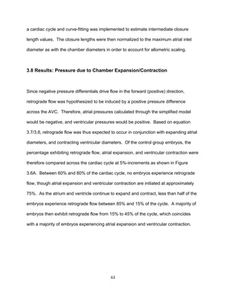


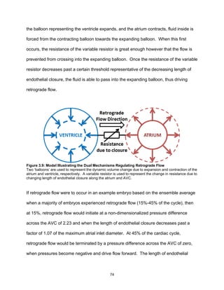
![75
closure would have decreased to a factor of 0.31 of the maximum atrial inlet diameter at
this point. Using an estimated viscosity of 4 cP (based on an average estimated in
previous embryonic zebrafish intracardiac flow studies) [8, 9, 107], the pressure at the
time retrograde flow would be initiated would translate to 0.152 μmHg.
One major limitation of this study was that flow could not be measured at the AVC,
which would have allowed for calculation of resistance due to closure and shear stress
on the endocardial cushions. Because the AVC is constricted for a majority of the
cardiac cycle, the diameter on the focal plane in-view is only on the order of a few pixels
and thus too low to measure accurately. Since spatiotemporal analysis of the flow
through KAT software assumes a circular profile, which squares diameter values, and
because resistance calculations are derived from the diameter to the fourth power, flow
rates at the AVC cannot be measured with any accuracy. The use of proportional
parameters such as the length of endothelial closure provide an understanding of the
mechanisms influencing retrograde flow, though to determine exact values of
parameters necessary to generate retrograde flow would require further analysis using
more resolute imaging modalities.
The circular-profile assumption of the KAT software also limits the accuracy of pressure
calculations in the chambers. A cylindrical control volume within the heart was used to
estimate chamber volume due to its compatibility with the circular-profile assumption of
the software. Not only are the chambers not of a circular profile, which will be further
discussed in Aim 2 of this thesis, but during contraction, the chambers likely undergo](https://image.slidesharecdn.com/b9d15e8e-7423-429a-9418-53bc61f3c1fa-160106203545/85/Bulk_Alexander_Thesis-85-320.jpg)
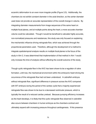

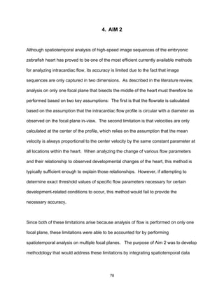
![79
from multiple focal planes into more accurate intracardiac flow data. A complementary
algorithm to the KAT (Kymograph Analyzation Tool) software developed by Johnson, et
al. [109] as described in the literature review was created in MATLAB (Mathworks, Inc.)
that uses diameter and velocity data on each focal plane to recalculate both the profile
area, and velocity profile across a cardiac cycle. By recalculating these two
parameters, flow rate as well as additional parameters descriptive of cardiac function
were able to be estimated with reduced error in comparison to the previous
methodology.
4.1 Methods: Zebrafish Embryo Preparation and Imaging
Wildtype zebrafish were raised and bred in accordance with Westerfield [112] in the
same manner as described in the methods section for Aim 1 (Chapter 3.2). Embryos
were stored at the same temperature and in the same solution of E3 media with
methylene blue trihydrate (0.5 g/L) until imaging was performed at 55 hpf. In order to
maximize the number of focal planes used for analysis of intracardiac flow, the time
point of 55 hpf was used because at this point, the heart has increased to its maximum
girth prior to the onset of pigmentation. Since an experimental group with altered
cardiac preload was not required as in Aim 1, dechorionation was not conducted on the
embryos until imaging at 55 hpf. Between 48 hpf and 55 hpf, most embryos “hatch”
from their chorion independently, so it was however only necessary for a few embryos
to be dechorionated. Dechorionation was again performed manually using forceps and
tweezers.](https://image.slidesharecdn.com/b9d15e8e-7423-429a-9418-53bc61f3c1fa-160106203545/85/Bulk_Alexander_Thesis-89-320.jpg)
![80
In order to capture high-speed image sequences of the heart on multiple focal planes,
each image sequence was taken independently of one another in consecutive order
using the same Photron FASTCAM SA3 high-speed camera used in Aim 1. In Aim 1 as
well as in previous studies [50], a frame rate of 1500 frames per second was used,
which would result in download times ranging between 15 and 20 minutes. Since
embryos needed to remain perfectly still throughout the process of capturing each
image sequence, this download time was far too long, as embryos would twitch before
being able to capture image sequences on only the first few focal planes. Fortunately,
this temporal resolution was far greater than necessary in order to accurately calculate
velocity based on radon transforms across ST plots as described in the literature
review. By reducing the frame rate to 1000 frames per second, the download time was
reduced to just over 2 minutes, which allowed for all embryos to be analyzed on each
focal plane before any movement would occur. This frame rate was determined to be
the best option for analysis, as it could have been further reduced before any
detrimental effect on the velocity calculations would be induced. Also, the same
Olympus SZX12 bright-field stereomicroscope was used as in Aim 1, though with a
spatial resolution of 1,024 pixels per millimeter.
One primary method to determine the accuracy of any computational flow-measurement
software is through calculating the difference in downstream flowrate. Due to the
cyclical nature of intracardiac flow, the difference in downstream stroke volume (ΔSV)
was thus compared between the multi-focal plane and circular-profile methods of
spatiotemporal analysis:](https://image.slidesharecdn.com/b9d15e8e-7423-429a-9418-53bc61f3c1fa-160106203545/85/Bulk_Alexander_Thesis-90-320.jpg)
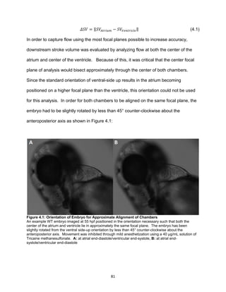
![82
Though it may have been possible to create a divot in a layer of agarose gel in order to
position the embryo in the orientation described (Figure 4.1) as was the case in Aim 1, it
would have been extremely difficult to shape the divot manually using a dissecting razor
such that the embryo could easily fall into this orientation. Therefore, small drops of
melted agarose gel were injected at various locations on the petri dish and allowed to
solidify such that the embryo could lean up against the drops after being positioned next
to them ventral side-up. Despite the induced reduction in image sequence download
speed by lowering the frame rate, embryos would still have the tendency to twitch in this
position before sequences on each focal plane could be acquired. To account for this,
mild anesthetization was induced by applying a 40 µg/mL solution of Tricaine
methanesulfonate to the E3 media in which the embryos were stored in and imaged
from. Because the purpose of this aim was merely to develop methodology to more
accurately quantify heart function, rather than analyze heart function in wildtypes, it was
not necessary for the embryos to maintain a normal heart rate [72], and thus the use of
Tricaine was permissible. This orientation was only necessary in order to calculate the
difference in stroke volume analyzed between the atrium and ventricle, so future use of
this methodology would not be limited to using Tricaine to position the embryos, and
could be used for analysis at many various orientations.
Based on the size of the chambers and depth of the focal plane, it was determined that
the optimal number of focal planes used for analysis across the heart was 5. The
average chamber diameter measured from image sequences of 42 wildtype embryos
saved from previous studies was approximately 112 µm, which translated to a distance](https://image.slidesharecdn.com/b9d15e8e-7423-429a-9418-53bc61f3c1fa-160106203545/85/Bulk_Alexander_Thesis-92-320.jpg)
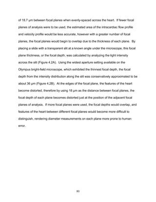


![86
integrated together into an estimated shape of the intracardiac flow profile. By
collecting diameter data from each focal plane at each time step across the cardiac
cycle, a profile area is able to be calculated at each time step to more accurately
calculate flowrate across the cycle. After image sequences of the embryonic heart are
captured on each focal plane, the region used to crop out the heart in the KAT software
is saved so that the same region can be used to crop out the heart in the image
sequences from the adjacent focal planes. The same is done with the reference lines
used to measure diameter and velocity so the exact same region along the x-y plane is
measured on every focal plane. When measuring diameter using KAT, careful attention
is paid when selecting diameter points so that diameters from the outermost interior
diameter are not selected when blurred and out-of-plane, and that only points on
endothelial cells along the edge of the heart that are clearly visible are selected.
When diameter data is integrated together, the orientation of the points along the edge
of the diameters with respect to each other is not saved from the original KAT analysis.
Therefore, the diameters points are oriented such that their centers are aligned on the
z-axis, producing a parallel shape. Though this affects the estimated shape of the edge
of the profile, it does not affect the estimated area due to Cavalieri’s Principle.
Cavalieri’s Principle states that if two regions in a plane are bisected by line segments
of equal length, then the regions have equal areas [115]. Therefore, since the
measured diameters can be treated as line segments and the intracardiac flow profile
the plane, the estimated area between the diameters will be unaffected by their
orientation with respect to each other. By generating an estimated curvature around the](https://image.slidesharecdn.com/b9d15e8e-7423-429a-9418-53bc61f3c1fa-160106203545/85/Bulk_Alexander_Thesis-96-320.jpg)
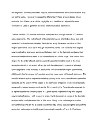


![90
With each spline segment polynomial generated, the area of the intracardiac profile, A(t)
is then able to be calculated by taking the definite integral of each spline segment
polynomial, Sm between the points θm-1 and θm:
𝐴(𝑡) = ∑ ∫ [𝑎𝑖 𝜑3
+ 𝑏𝑖 𝜑2
+ 𝑐𝑖 𝜑 + 𝑑𝑖]𝜕𝜑
𝜃 𝑖
𝜃 𝑖−1
𝑚
𝑖=1 (4.8)
The result of generating polar spline segments to calculate area from a set of five test
diameters based on the set of polar spline segments in Figure 4.3 is shown below in
Figure 4.4.
Figure 4.4: Area Calculation of the Intracardiac Flow Profile and Associated Error Resolution
A: Ten polar spline segments (black, S1-S10) were generated from points on the outer edge of the five
test diameters (red, D1-D5) from Figure 4.3. B: Area calculation using definite integrals of the polar spline
segment polynomials is illustrated using different colored regions representing the area calculated across
each individual segment. Blue lines are used to represent the limits of each definite integral. C: When a
point is excluded from polar spline segment generation, occasionally the spline segment will pass beyond
that point, resulting in an overestimated area. By forcing the spline segments to pass through that point,
a more accurate area estimation is obtained.
Occasionally, when diameters less than 1 µm are excluded from polar spline segment
generation, the spline segments will pass beyond that focal plane, resulting in an](https://image.slidesharecdn.com/b9d15e8e-7423-429a-9418-53bc61f3c1fa-160106203545/85/Bulk_Alexander_Thesis-100-320.jpg)

![92
analysis is addressed. As discussed in the literature review, the mean velocity was
determined to be proportional to the measured center velocity by a factor of 0.74, which
was determined through analysis of the flow profile at only one region of the heart [55].
This may not be the case at all regions of the heart, and during all times throughout the
cardiac cycle, therefore by using multiple velocities on multiple focal planes, the mean
velocity can be generated through an estimated velocity profile at each time point
across the cardiac cycle. To generate a velocity profile, a Riemann sum is taken of the
velocities along the z axis across focal planes (Figure 4.5).
Figure 4.5: Mean Velocity Calculation of the Intracardiac Flow Profile through Riemann Sums
To calculate mean velocity at each time step across the cardiac cycle, rectangles are generated with an
area equivalent to the product of the velocity at the z-axis position within that rectangle and the width of
the rectangle along the z-axis. Endpoints of each rectangle on the z-axis are set at the midpoints
between the z-axis positions of the focal planes of each velocity (red dots), and the outermost endpoints
of rectangles 1 and 5 (blue dots) are determined from the position of the radius of the generated polar
spline segments (Figure 4.4). The distance between the outermost endpoints is divided from the sum of
the rectangles to estimate the mean velocity of the flow profile.
The endpoints of each rectangle along the z axis are at the midpoints between each
focal plane of analysis, and the outer endpoints of the outermost rectangles are](https://image.slidesharecdn.com/b9d15e8e-7423-429a-9418-53bc61f3c1fa-160106203545/85/Bulk_Alexander_Thesis-102-320.jpg)
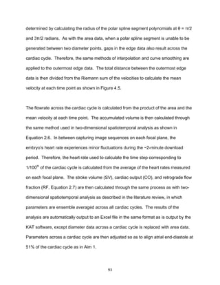
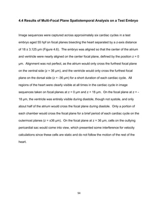
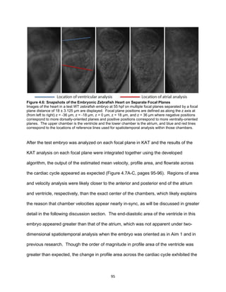
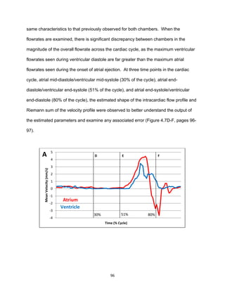

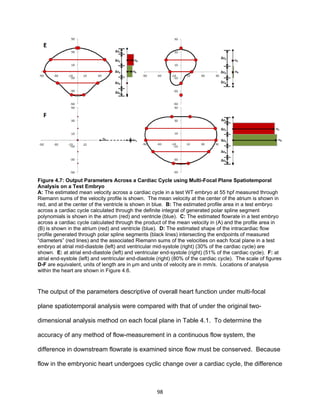


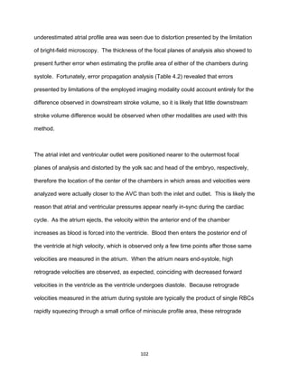
![103
velocities translated to retrograde flowrates only on the order of a few picoliters per
minute.
The average ratio of the mean velocity to the maximum velocity was measured in order
to compare with the ratio used to calculate mean velocity from the centerline velocity in
2-D spatiotemporal analysis of 0.74. In the test embryo, this ratio was calculated to be
0.528, which is much closer to the ratio of 0.5 typically observed in laminar flow-
conditions. This is also what would be expected based on the observed shape of the
intracardiac flow profile during diastole shown in Figures 4.7D, E, and F. At all time-
points during diastole, the width along the z-axis of the intracardiac flow profile in each
chamber was greater than the width observed along the x-y plane. Therefore, it makes
sense that the ratio of mean velocities measured along the x-y plane to the centerline
velocity was greater than the same ratio of mean velocities measured along the z-axis.
Though a parabolic velocity profile is characteristic of flow under these conditions,
velocities were observed to be significantly greater at the center of the chamber than on
the outermost focal planes, which would often detect no velocity throughout the cardiac
cycle. The velocity profile in the zebrafish embryo heart has not been analyzed using
other flow-measurement methods, however the profile in the forming vessels has been
shown to exhibit a blunted parabolic profile due to the low shear stress in the center of
the vessel [116]. This is likely the case in the center of the chambers of the forming
heart as well.](https://image.slidesharecdn.com/b9d15e8e-7423-429a-9418-53bc61f3c1fa-160106203545/85/Bulk_Alexander_Thesis-113-320.jpg)

![105
The overall magnitude of the estimated flowrate across the cardiac cycle was far greater
in the ventricle than measured in the atrium, resulting in the 0.467 nL difference in
stroke volume measured between chambers shown in Table 4.1. Because mean
velocities in the atrium and ventricle were of relatively similar magnitude throughout the
cardiac cycle, this discrepancy in flowrate was likely the result of error in the estimated
profile area. Maximum flowrates in the ventricle occurred during ventricular diastole
(since analysis of the ventricle was closer to the AVC than the center of the ventricle),
however upon examination of the estimated flow profile at ventricular end-diastole
(Figure 4.7F), it does not appear that an irregular profile shape was being generated
that would result in a significantly overestimated area. Rather, it could be that profile
areas of the atrium were underestimated during end-diastole and ejection, when
maximum atrial velocities were observed and would have otherwise resulted in
flowrates near that observed in the ventricle. The estimated profile area of the atrium at
mid and end-diastole (Figure 4.7D-E) show that the measured “diameters” of the atrium
on the dorsal side of the heart were much less than those of the center plane and on the
ventral side, resulting in an irregular profile shape resembling a reflector light bulb. This
was quite unlike the shape suggested by the bean-shaped outer myocardial morphology
revealed by confocal images captured in previous studies [34]. Because of this irregular
shape, it is likely that the “diameters” measured on those focal planes were
underestimated due to some distortion of the heart on one side of the atrium that
prevented red blood cells flowing across those planes from appearing in focus. Since
careful detail was made to select only in-focus features of the heart as diameter points,
these distorted features that were likely actually in-plane were assumed to be out-of-](https://image.slidesharecdn.com/b9d15e8e-7423-429a-9418-53bc61f3c1fa-160106203545/85/Bulk_Alexander_Thesis-115-320.jpg)
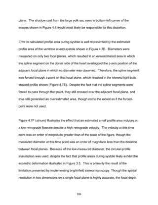
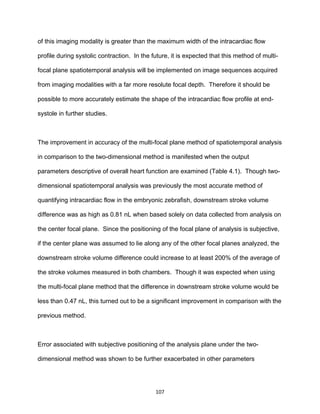
![108
descriptive of heart function, especially in retrograde flow fraction. On nearly all focal
planes as well as with the multi-focal plane method, retrograde flow fractions never
exceeded 3% except on the outermost focal plane on the ventral side of the heart. On
this plane, the retrograde flow fraction was nearly as high as 44%, which likely was the
result of interference in velocity measurements caused by cells on the pericardial sac.
Since those cells do not follow the motion of the heart, it is likely that the movement of
the heart in reference to these cells caused them to be analyzed as if they were red
blood cells flowing in retrograde, resulting in erroneously large retrograde flowrates.
One limitation of the two-dimensional method of spatiotemporal analysis that has not
been addressed in the multi-focal plane method is that only the in-plane component of
the velocity on each plane is measured, as illustrated in Figure 4.8. Therefore, the
mean velocity and flowrate are likely significantly underestimated since they do not take
into account the out-of-plane component, which likely contributes to the overall
downstream error in stroke volume. Methods have been developed to calculate out-of-
plane velocities in PIV systems by measuring both the increase in diameter and
decrease in intensity of particles as they move away from the focal plane [117, 118].
Unfortunately, the density of red blood cells in the embryonic zebrafish heart is too great
for the change in size and intensity of each cell to be distinguishable as they move out-
of-plane, as too many other RBCs would obstruct their view. Out-of-plane velocities
could be measured by capturing image sequences on focal planes bisecting the heart at
various different angles by simply rotating the embryo. Not only would this drastically](https://image.slidesharecdn.com/b9d15e8e-7423-429a-9418-53bc61f3c1fa-160106203545/85/Bulk_Alexander_Thesis-118-320.jpg)