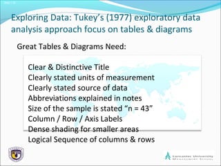
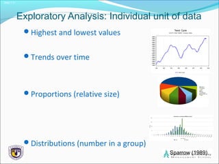
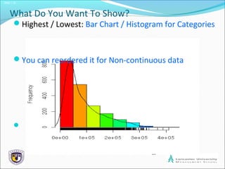
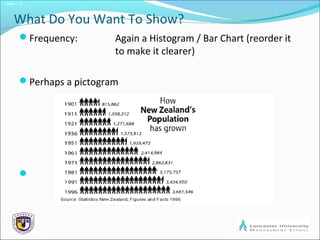
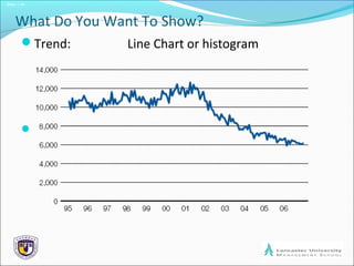
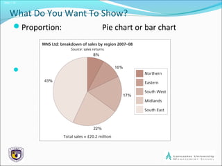
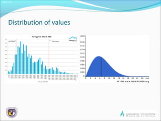
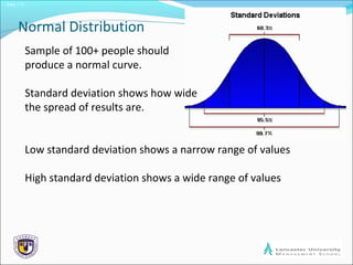
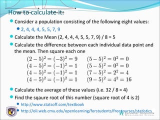
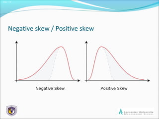
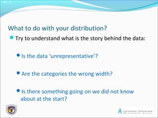
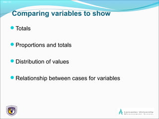
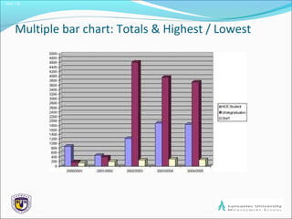
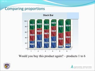
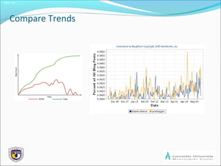
The document discusses quantitative data analysis, emphasizing the need for data preparation, appropriate statistical methods, and use of computer software for analysis. It outlines types of data, methods for exploratory analysis, and visualization techniques such as charts and graphs. Additionally, it touches on concepts like normal distribution, standard deviation, and the importance of verifying data representation.

1. Slide 1.1
Analysing quantitative data

2. Slide 1.2
Quantitative data analysis
Key points
Data must be analysed to produce information
Computer software analysis is normally used for this
process (Microsoft Excel, SPSS etc.)
Present, explore, describe & examine relationships

3. Slide 1.3
Examples of basic chart
Pie chart
Saunders et al. (2009)
Figure 12.8 Pie chart

4. Slide 1.4
More advanced work requires Statistical analysis
Establishing the statistical relationship between two
variables (e.g. If I am in this group I am have a %
probability of doing X).
If you need to do this then see:
http://www.statsoff.com/textbook
http://oli.web.cmu.edu/openlearning/forstudents
/freecourses/statistics

5. Slide 1.5
Quantitative data analysis: Main Concerns
Preparing, inputting and checking data
Choosing the most appropriate statistics to
describe the data
Choosing the most appropriate statistics to
examine data relationships and trends

6. Slide 1.6
Type of Data: category data
 Example: Number of cars hatchback / saloon /
estate
 Can’t measure it, just simply count occurrences
 Focus on one discrete variable (i.e. Hatchback)
 Dichotomous data (e.g. either Male or Female)
 Ranked data (how strongly you agree with
statement X)

7. Slide 1.7
Type of Data: numerical data
 Example: temperature in Celsius
 Quantifiable data that can be measured
 Interval data e.g. Degrees Celsius [zero
degrees is not actually ZERO]
 Ratio (calculate the difference) data e.g.
Profits up 34% for a year

8. Slide 1.8
Type of Data: continuous data
 Example: height of students
 Can be any value [within a range]

9. Slide 1.9
Level of Precision
LESS MORE
Precise data can be grouped to make it less precise
(e.g. Mark of 85% grouped into a ‘Very Good’ category but
Not the other way round)

10. Slide 1.10
Exploring Data: Tukey’s (1977) exploratory data
analysis approach focus on tables & diagrams
Great Tables & Diagrams Need:
Clear & Distinctive Title
Clearly stated units of measurement
Clearly stated source of data
Abbreviations explained in notes
Size of the sample is stated “n = 43”
Column / Row / Axis Labels
Dense shading for smaller areas
Logical Sequence of columns & rows

11. Slide 1.11
Exploratory Analysis: Individual unit of data
Highest and lowest values
Trends over time
Proportions (relative size)
Distributions (number in a group)
Sparrow (1989)

12. Slide 1.12
What Do You Want To Show?
Highest / Lowest: Bar Chart / Histogram for Categories
You can reordered it for Non-continuous data


13. Slide 1.13
What Do You Want To Show?
Frequency: Again a Histogram / Bar Chart (reorder it
to make it clearer)
Perhaps a pictogram


14. Slide 1.14
What Do You Want To Show?
Trend: Line Chart or histogram


15. Slide 1.15
What Do You Want To Show?
Proportion: Pie chart or bar chart


16. Slide 1.16
Distribution of values

17. Slide 1.17
Normal Distribution
Sample of 100+ people should
produce a normal curve.
Standard deviation shows how wide
the spread of results are.
Low standard deviation shows a narrow range of values
High standard deviation shows a wide range of values

18. Slide 1.18
How to calculate it:
Consider a population consisting of the following eight values:
2, 4, 4, 4, 5, 5, 7, 9
Calculate the Mean (2, 4, 4, 4, 5, 5, 7, 9) / 8 = 5
Calculate the difference between each individual data point and
the mean. Then square each one
Calculate the average of these values (i.e. 32 / 8 = 4)
Find the sqaure root of this number (square root of 4 is 2)
http://www.statsoff.com/textbook
http://oli.web.cmu.edu/openlearning/forstudents/freecourses/statistics

19. Slide 1.19
Negative skew / Positive skew

20. Slide 1.20
What to do with your distribution?
Try to understand what is the story behind the data:
Is the data ‘unrepresentative’?
Are the categories the wrong width?
Is there something going on we did not know
about at the start?

21. Slide 1.21
Comparing variables to show
Totals
Proportions and totals
Distribution of values
Relationship between cases for variables

22. Slide 1.22
Multiple bar chart: Totals & Highest / Lowest

23. Slide 1.23
Comparing proportions
Would you buy this product again? – products 1 to 6

24. Slide 1.24
Compare Trends

25. Slide 1.25
A final word of caution
GI-GO
Garbage In – Garbage Out