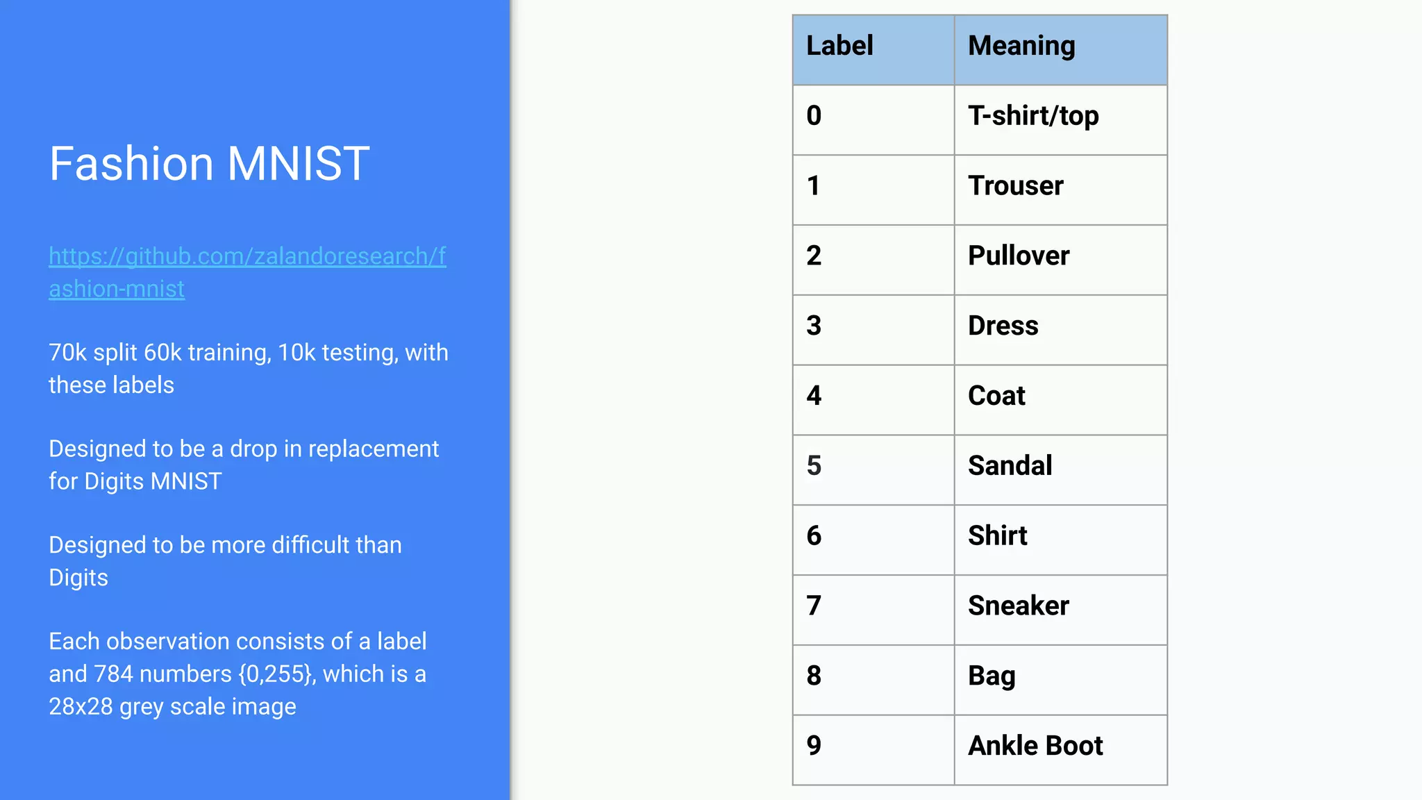
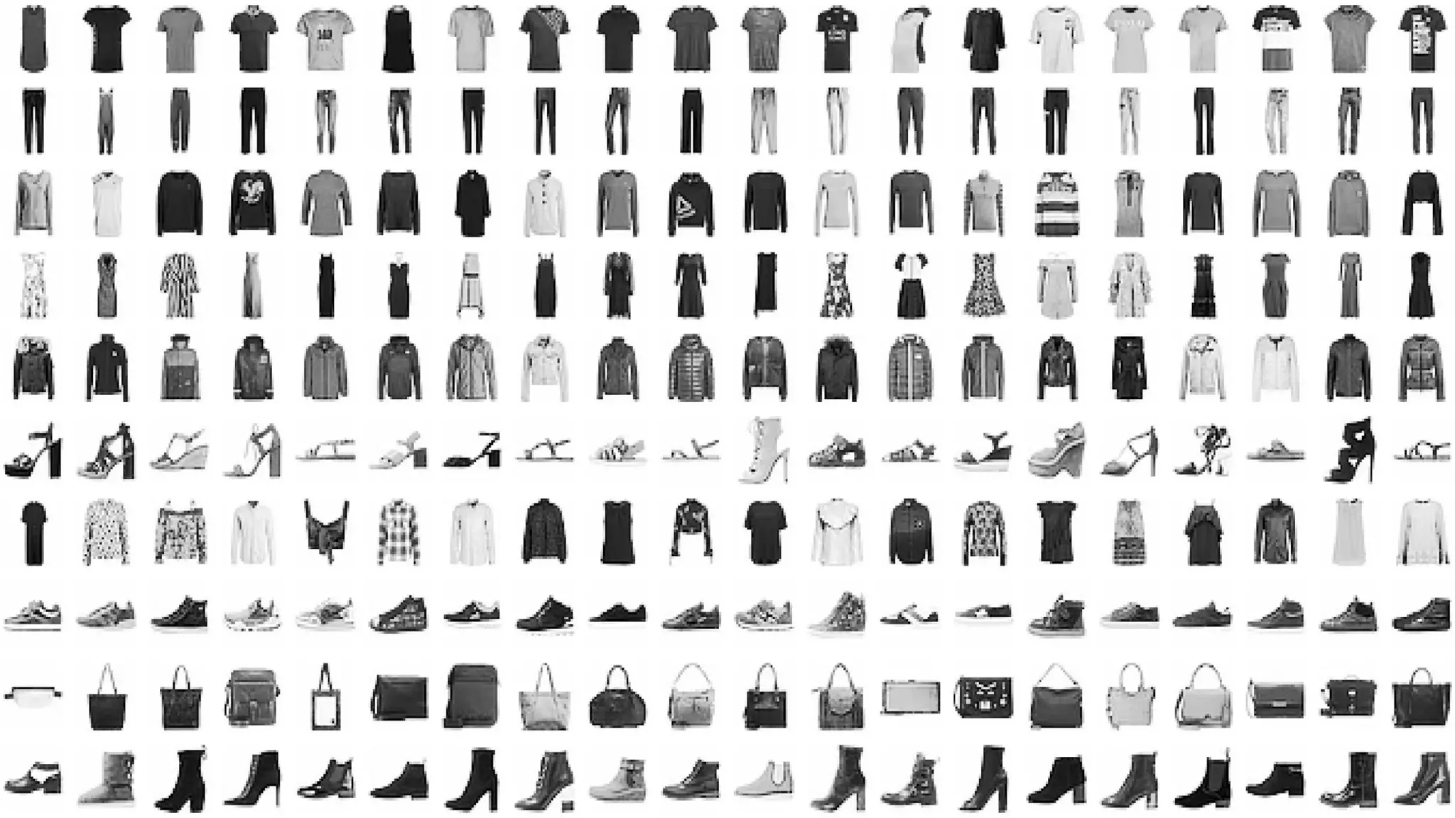
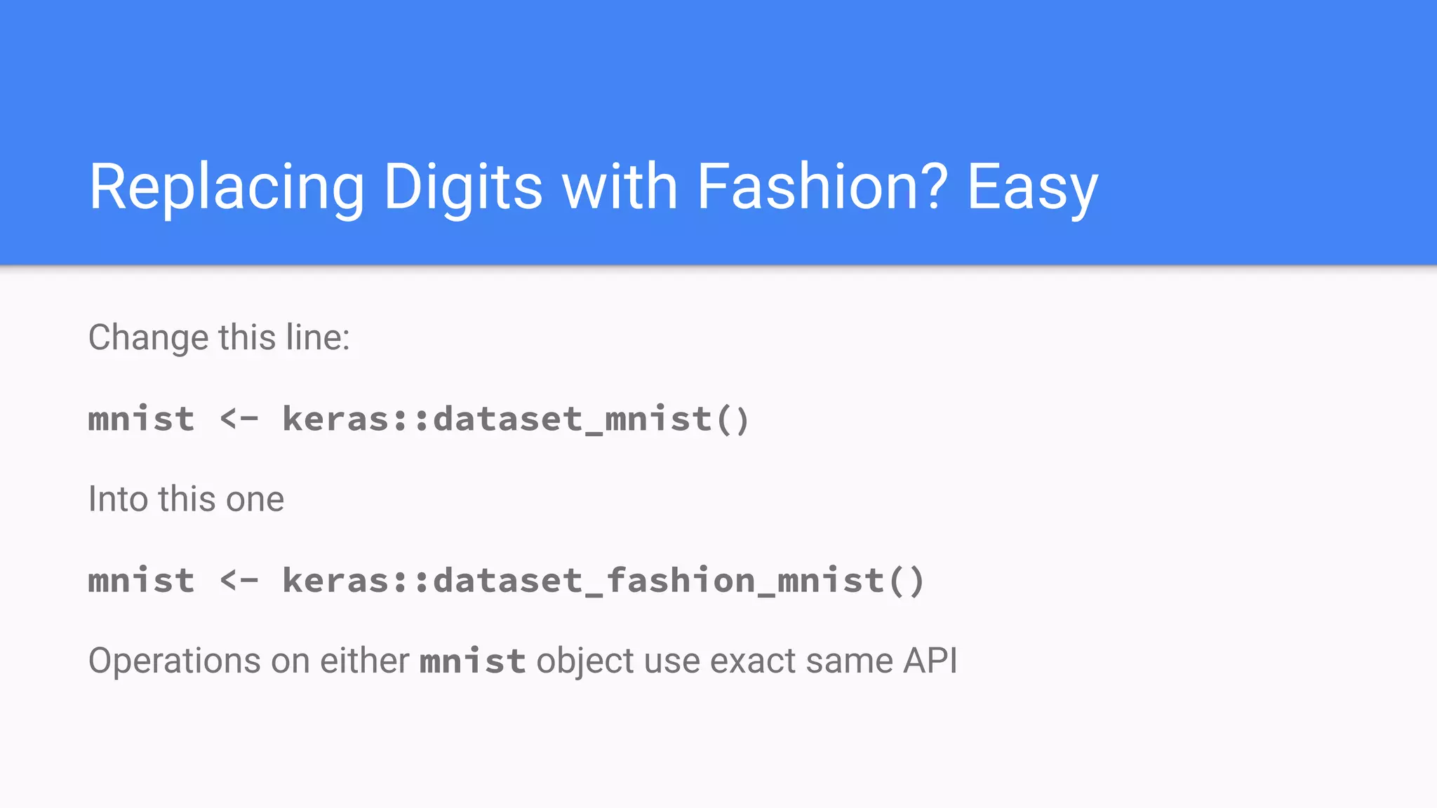
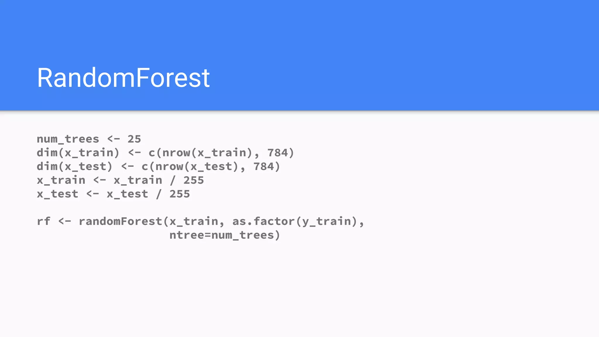
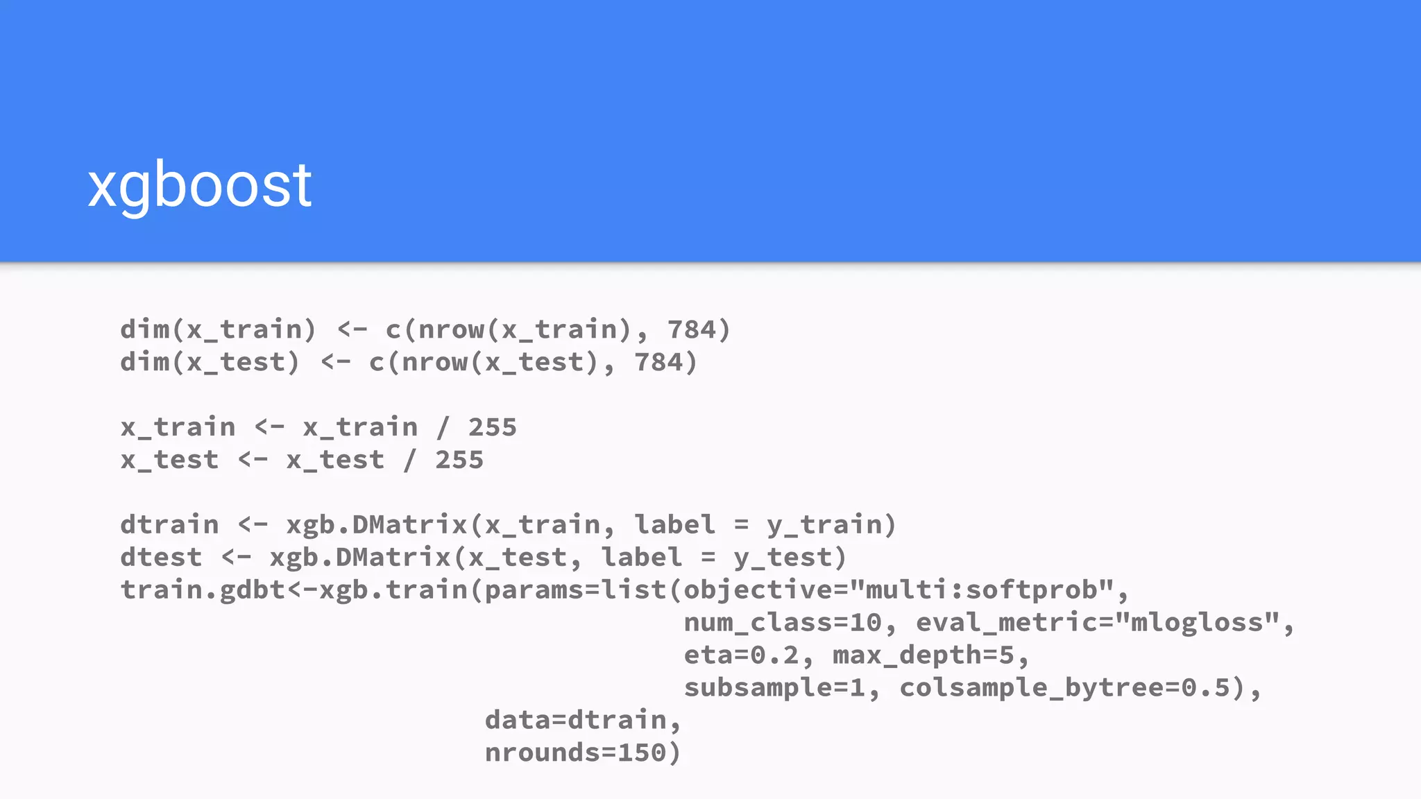
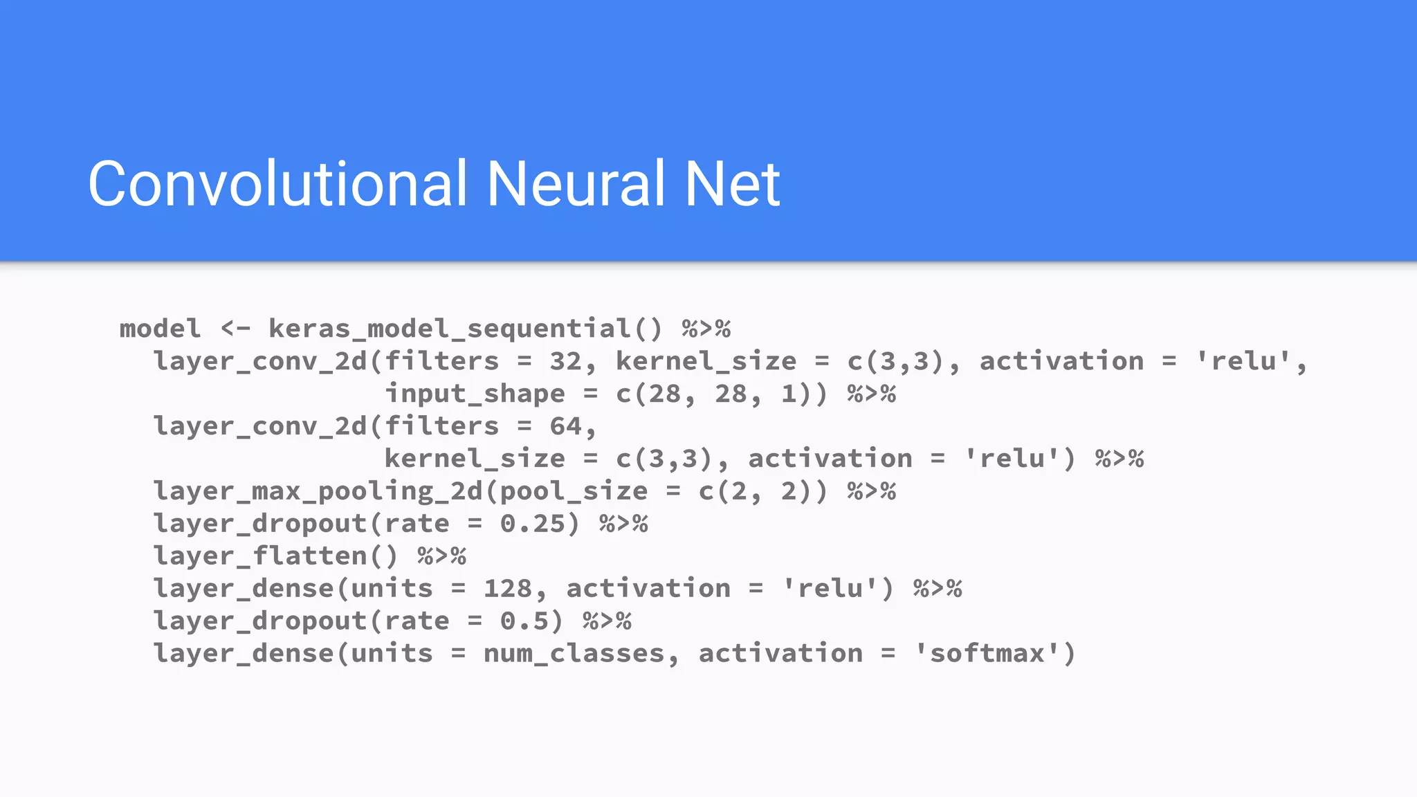
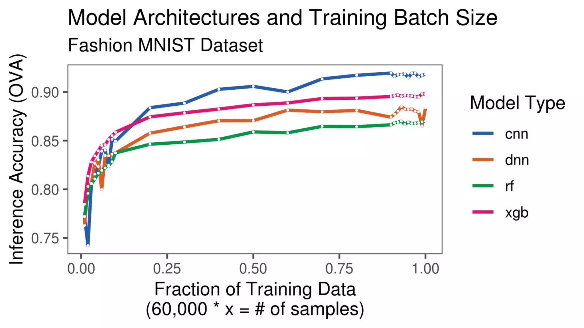
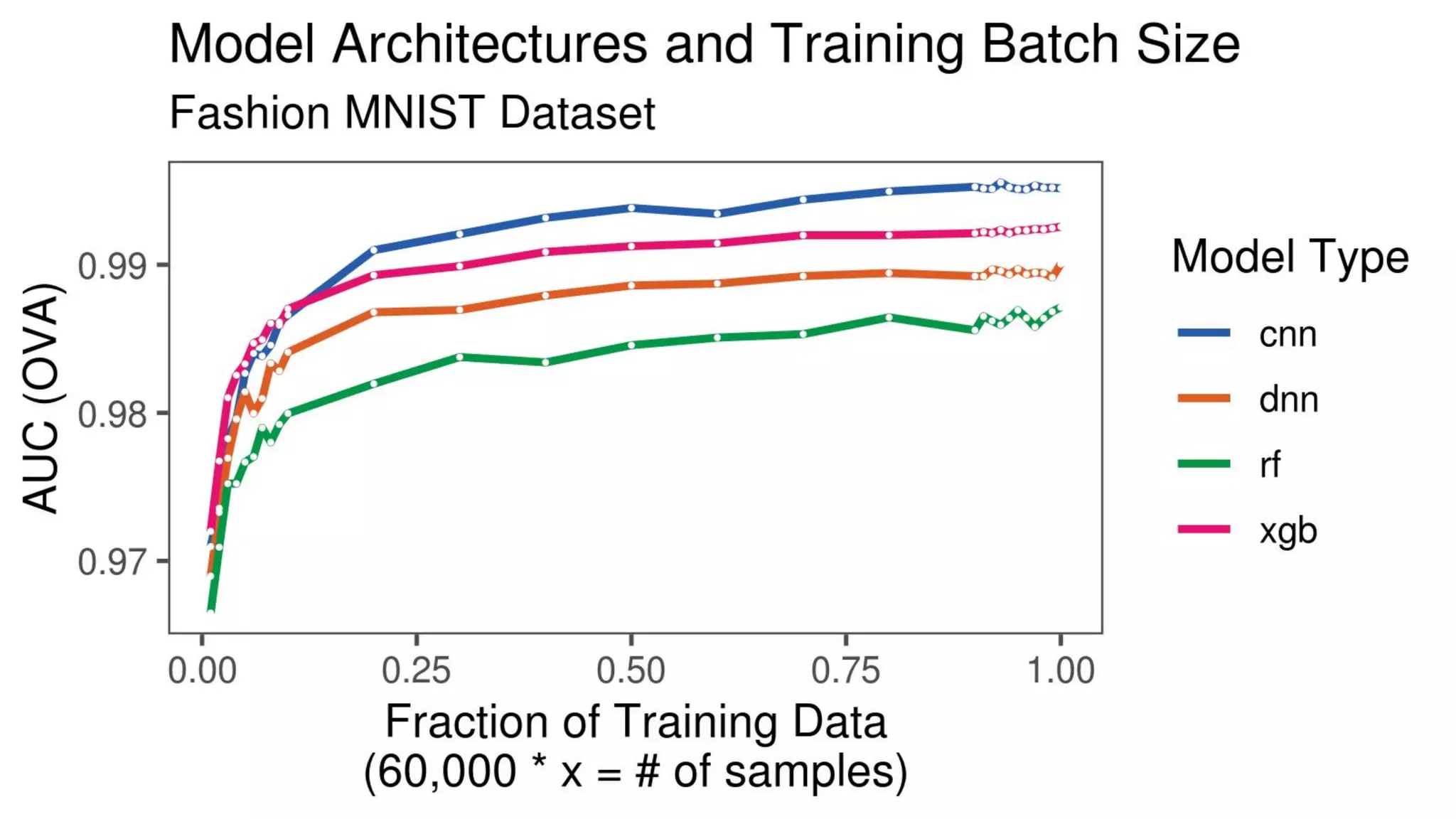
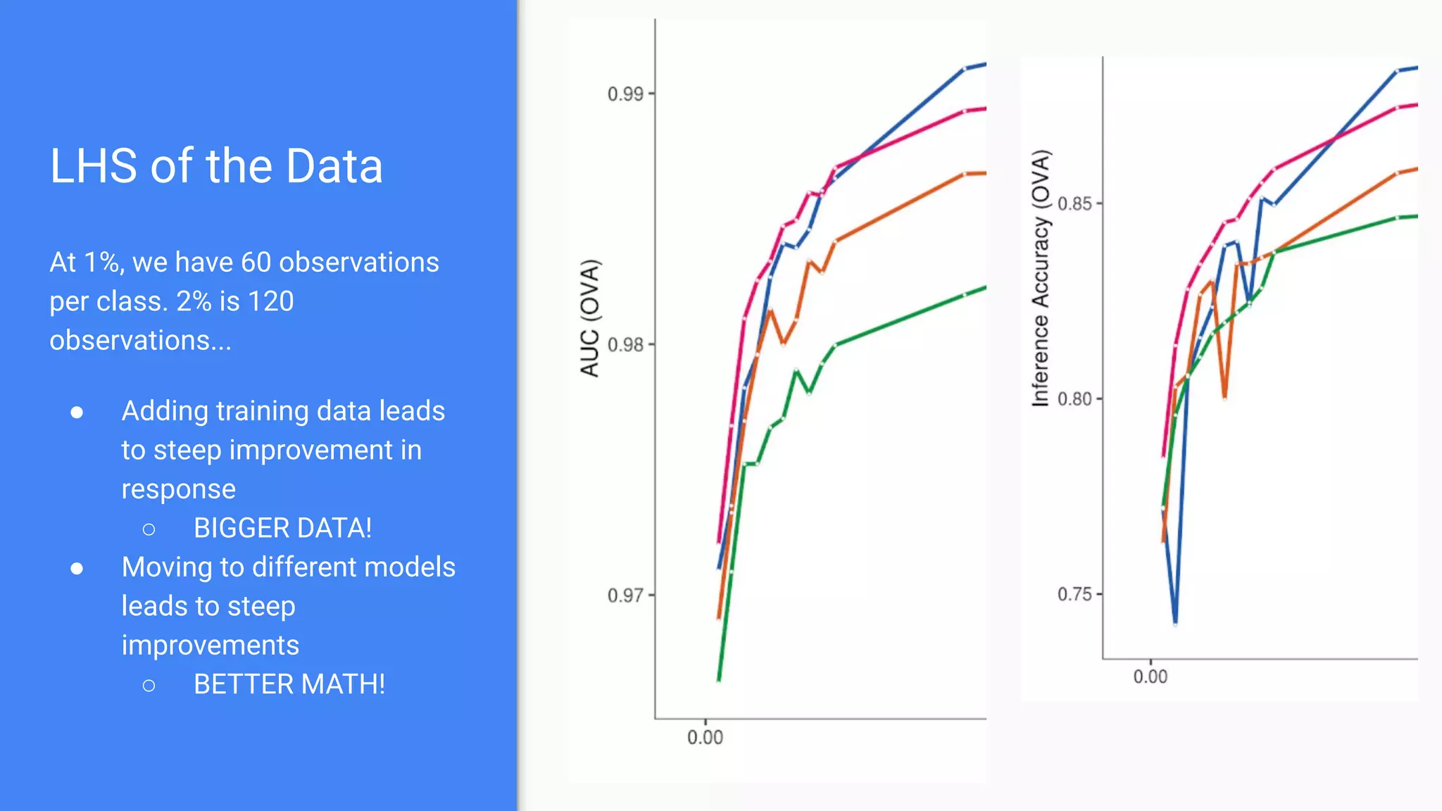
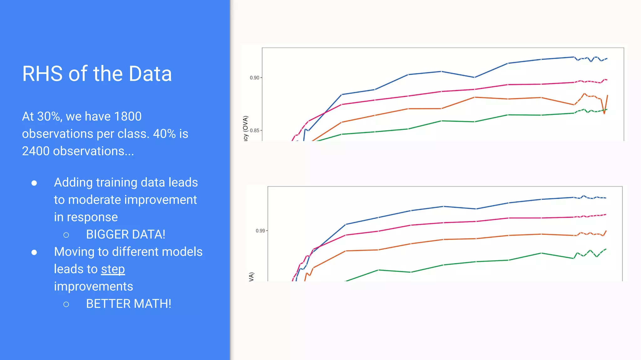
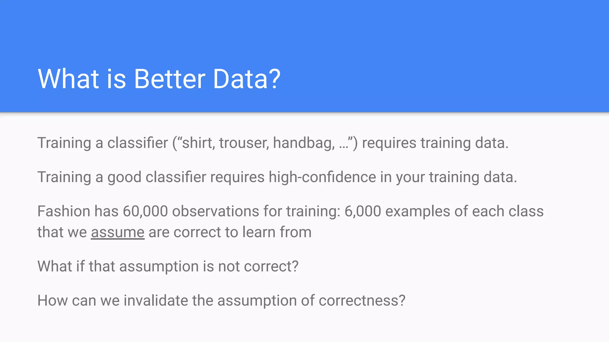
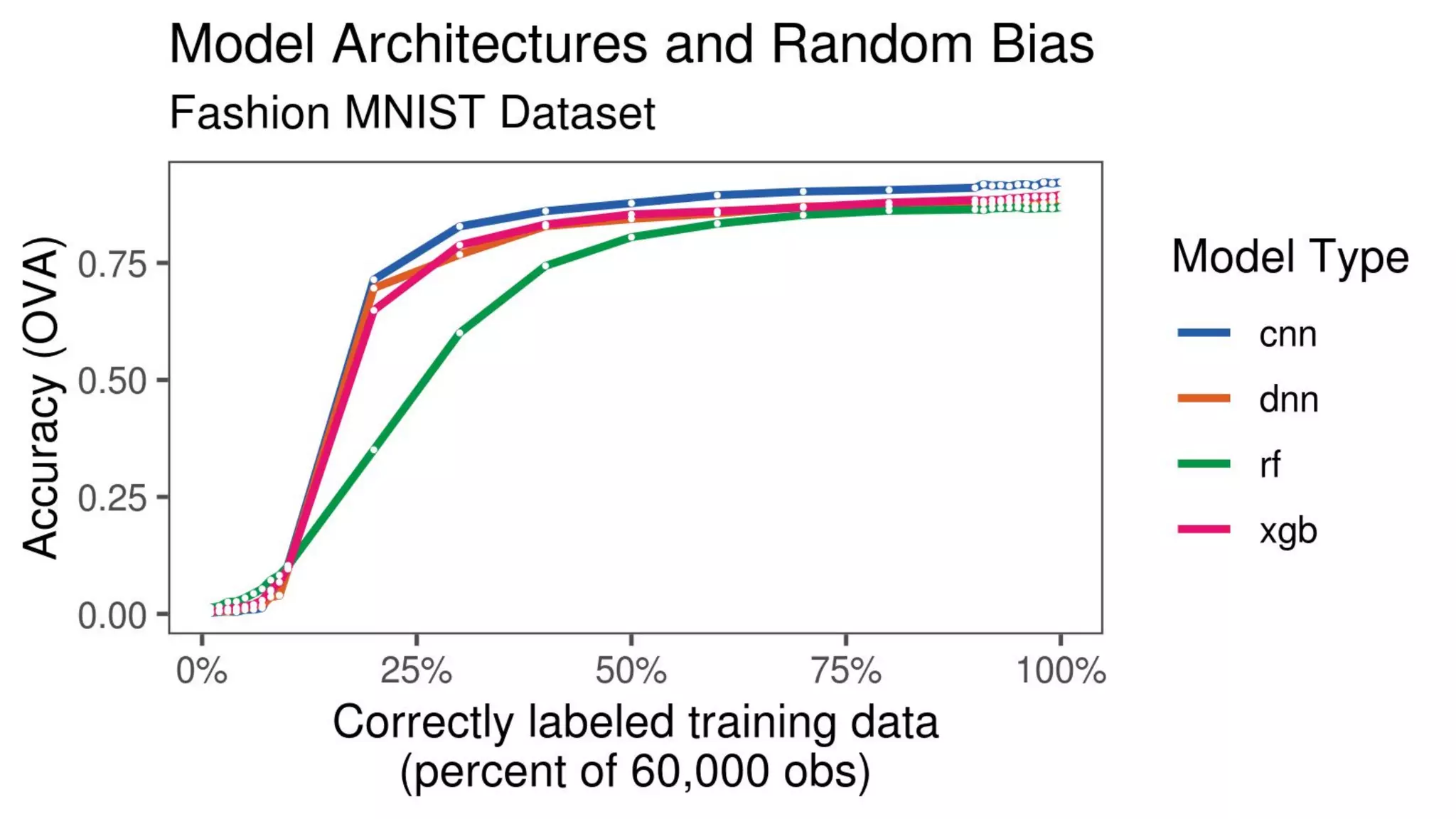
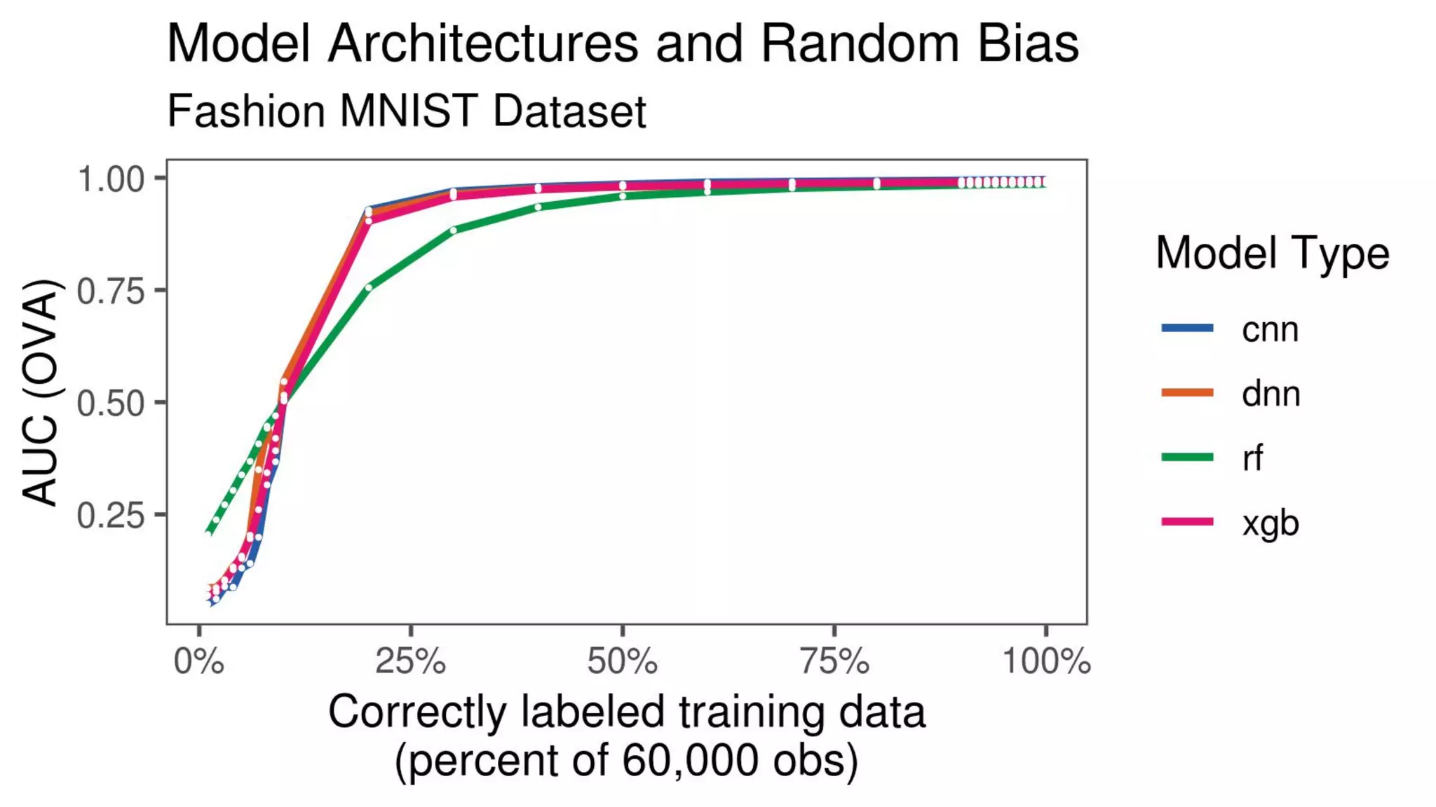
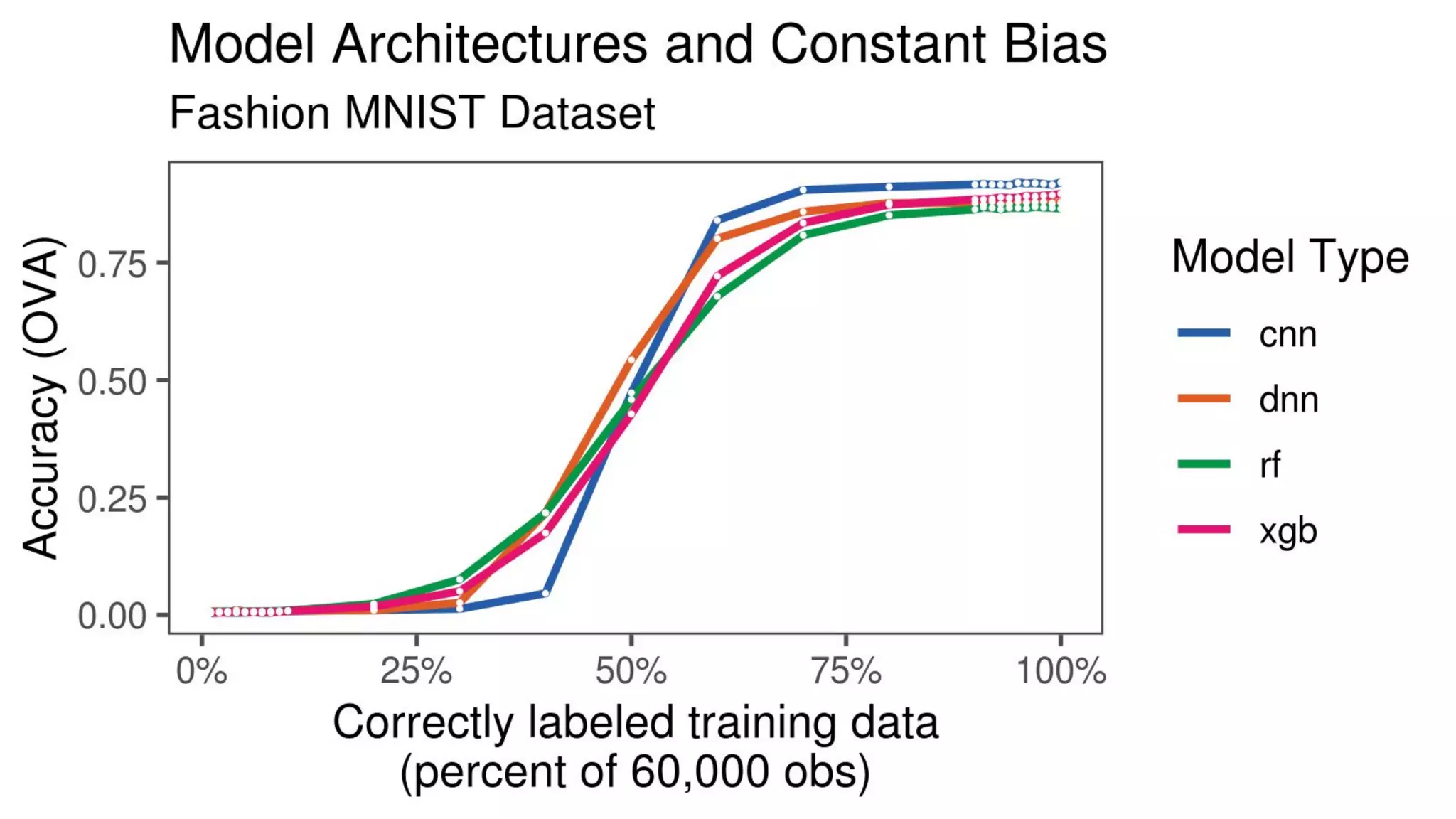
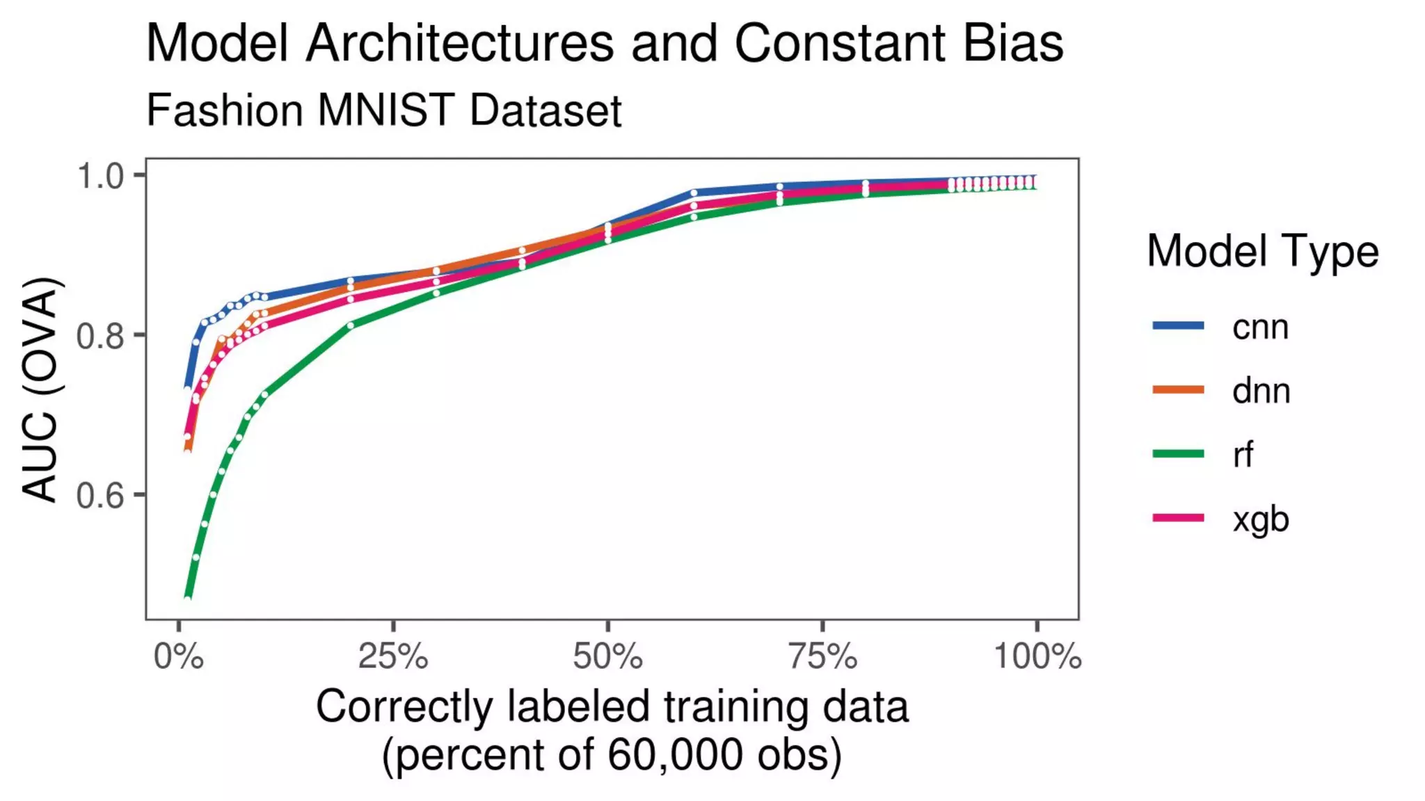
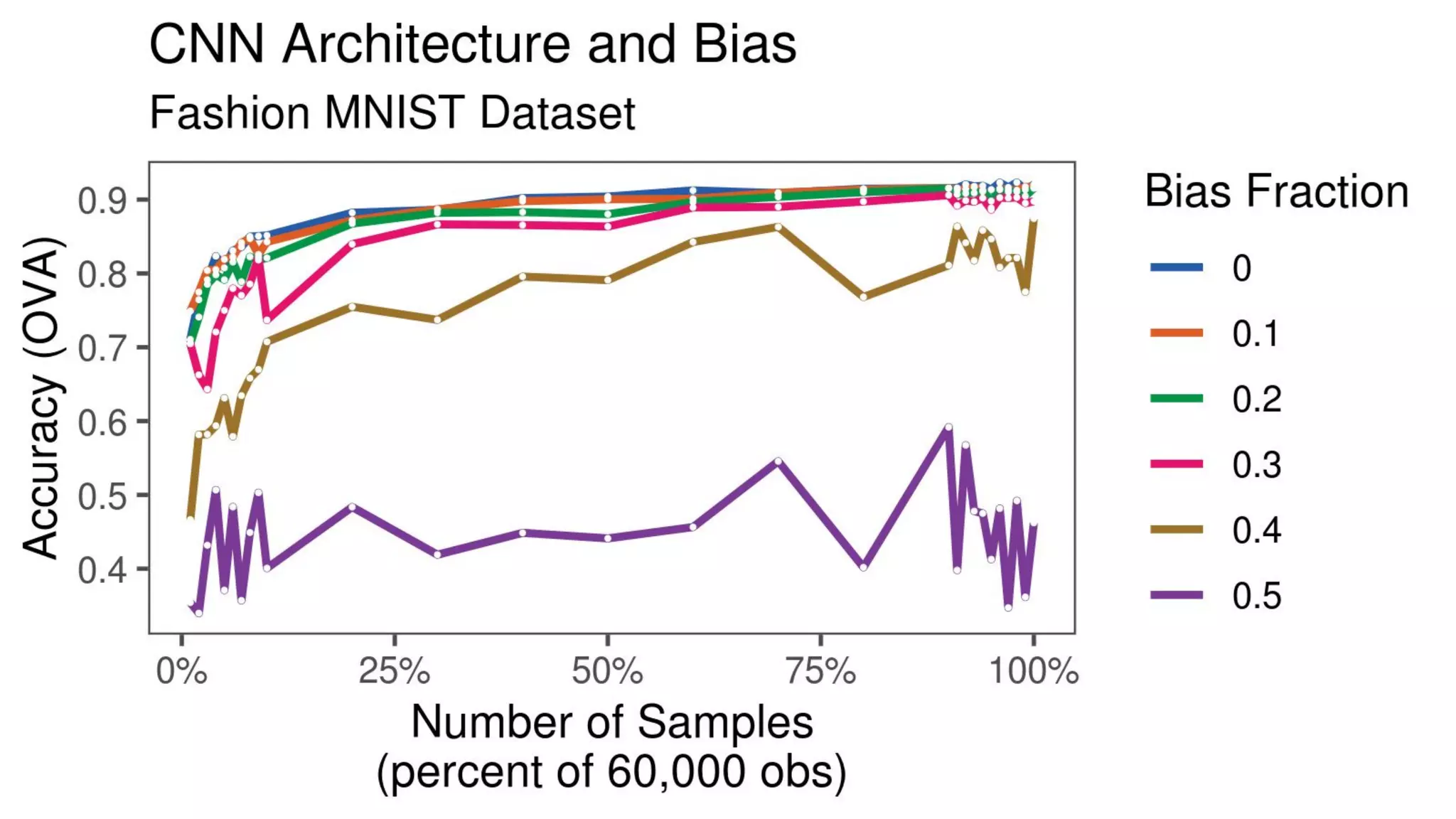
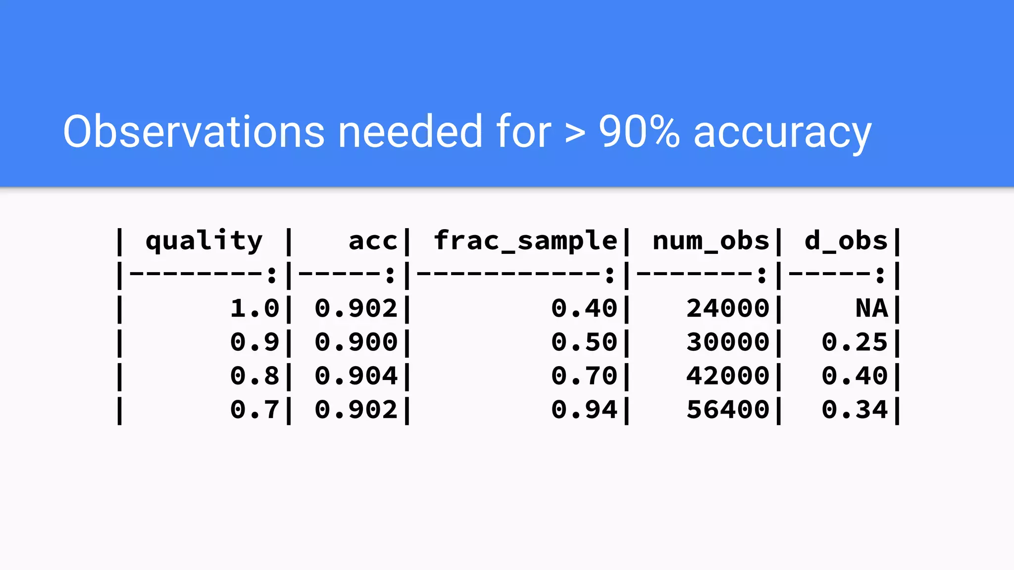
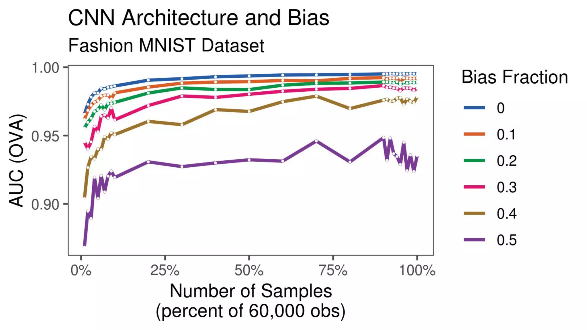
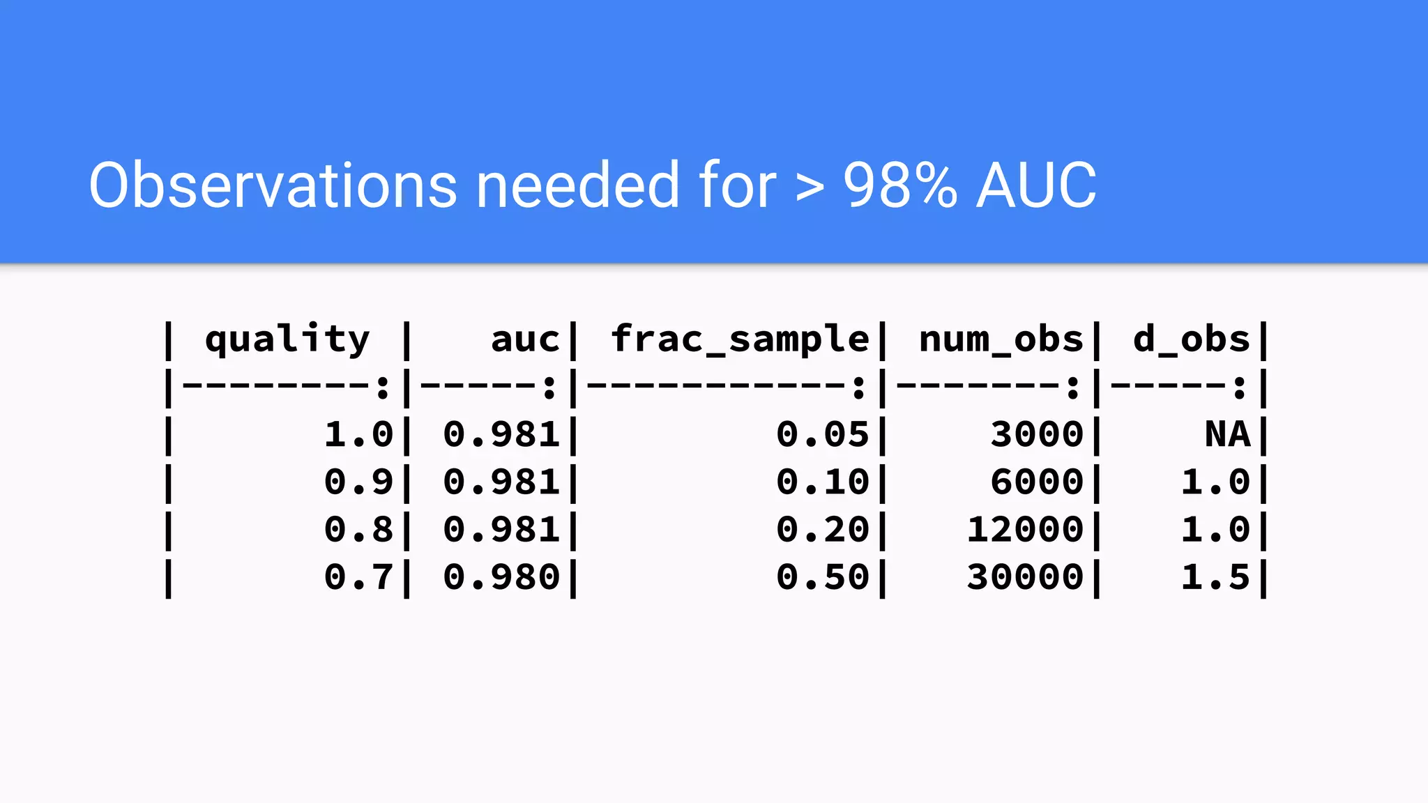
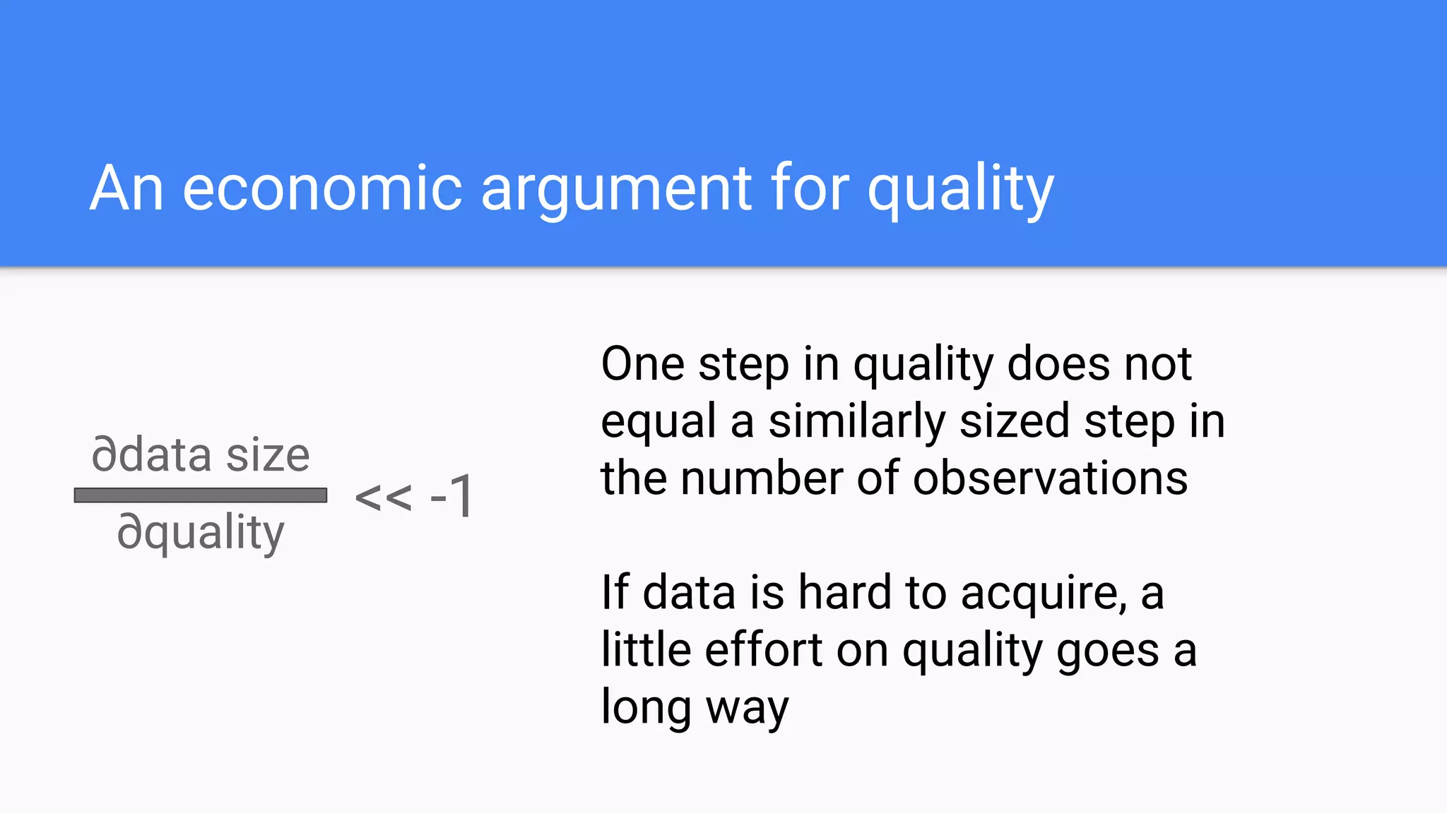
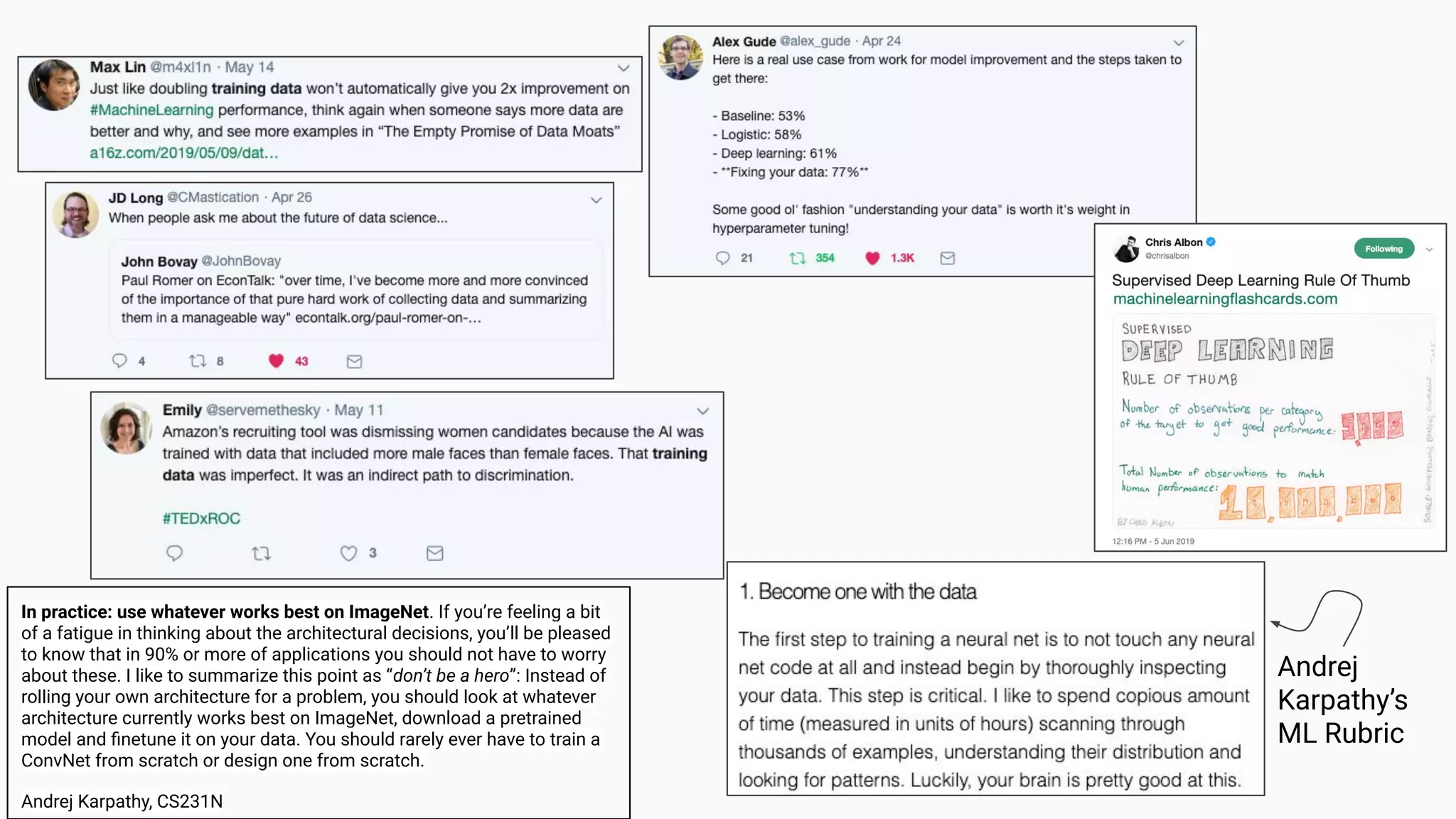
The document discusses the impact of using larger datasets versus different machine learning algorithms, concluding that bigger data significantly improves model performance, often more than switching models. It details experiments conducted on the Fashion MNIST dataset, illustrating how the amount of training data and the choice of model affect accuracy and AUC. The document also emphasizes the importance of data quality and encourages leveraging proven architectures rather than developing new ones from scratch.

1. “Bigger Data
Beats Better
Math, No
Question”

2. “If I invest in more
data, then the same
model will perform
better than switching
to a different ML
architecture ”

3. Bigger Data v Better Math
What has more impact in machine learning?
Brent Schneeman
@schnee

4. The Data

7. Fashion MNIST
https://github.com/zalandoresearch/f
ashion-mnist
70k split 60k training, 10k testing, with
these labels
Designed to be a drop in replacement
for Digits MNIST
Designed to be more difficult than
Digits
Each observation consists of a label
and 784 numbers {0,255}, which is a
28x28 grey scale image
Label Meaning
0 T-shirt/top
1 Trouser
2 Pullover
3 Dress
4 Coat
5 Sandal
6 Shirt
7 Sneaker
8 Bag
9 Ankle Boot

9. Replacing Digits with Fashion? Easy
Change this line:
mnist <- keras::dataset_mnist()
Into this one
mnist <- keras::dataset_fashion_mnist()
Operations on either mnist object use exact same API

10. And it looks like
> str(mnist)
List of 2
$ train:List of 2
..$ x: int [1:60000, 1:28, 1:28] 0 0 0 0 0 0 0 0 0 0 ...
..$ y: int [1:60000(1d)] 9 0 0 3 0 2 7 2 5 5 ...
$ test :List of 2
..$ x: int [1:10000, 1:28, 1:28] 0 0 0 0 0 0 0 0 0 0 ...
..$ y: int [1:10000(1d)] 9 2 1 1 6 1 4 6 5 7 ...

11. The Math

12. (these are not
great models, and
not greatly tuned)

13. RandomForest
num_trees <- 25
dim(x_train) <- c(nrow(x_train), 784)
dim(x_test) <- c(nrow(x_test), 784)
x_train <- x_train / 255
x_test <- x_test / 255
rf <- randomForest(x_train, as.factor(y_train),
ntree=num_trees)

14. xgboost
dim(x_train) <- c(nrow(x_train), 784)
dim(x_test) <- c(nrow(x_test), 784)
x_train <- x_train / 255
x_test <- x_test / 255
dtrain <- xgb.DMatrix(x_train, label = y_train)
dtest <- xgb.DMatrix(x_test, label = y_test)
train.gdbt<-xgb.train(params=list(objective="multi:softprob",
num_class=10, eval_metric="mlogloss",
eta=0.2, max_depth=5,
subsample=1, colsample_bytree=0.5),
data=dtrain,
nrounds=150)

15. “Deep” Neural Net
model <- keras_model_sequential()
model %>%
layer_dense(units = 256, activation = 'relu', input_shape = c(784)) %>%
layer_dropout(rate = 0.4) %>%
layer_dense(units = 128, activation = 'relu') %>%
layer_dropout(rate = 0.3) %>%
layer_dense(units = 10, activation = 'softmax')

16. Convolutional Neural Net
model <- keras_model_sequential() %>%
layer_conv_2d(filters = 32, kernel_size = c(3,3), activation = 'relu',
input_shape = c(28, 28, 1)) %>%
layer_conv_2d(filters = 64,
kernel_size = c(3,3), activation = 'relu') %>%
layer_max_pooling_2d(pool_size = c(2, 2)) %>%
layer_dropout(rate = 0.25) %>%
layer_flatten() %>%
layer_dense(units = 128, activation = 'relu') %>%
layer_dropout(rate = 0.5) %>%
layer_dense(units = num_classes, activation = 'softmax')

17. So we have
The Data
and we have
The Math

19. The Test Bench
tib <- c(1:9 / 100, 1:9 / 10, 91:100 / 100) %>%
sort() %>%
map_dfr(run_size_exp, x_train, y_train, x_test, y_test)
Basically, train with 1%, 2%, 3%, …,10%, 20%, 30%, …, 98%, 99%, 100% of the
training data and infer against the test set and you get
frac,exp_name,acc,auc
0.01,rf,0.8291,0.9759206200228384
0.01,xgb,0.8513,0.9859652247914469
0.01,dnn,0.8491,0.9860249426097214
0.01,cnn,0.9018,0.9922435869596523

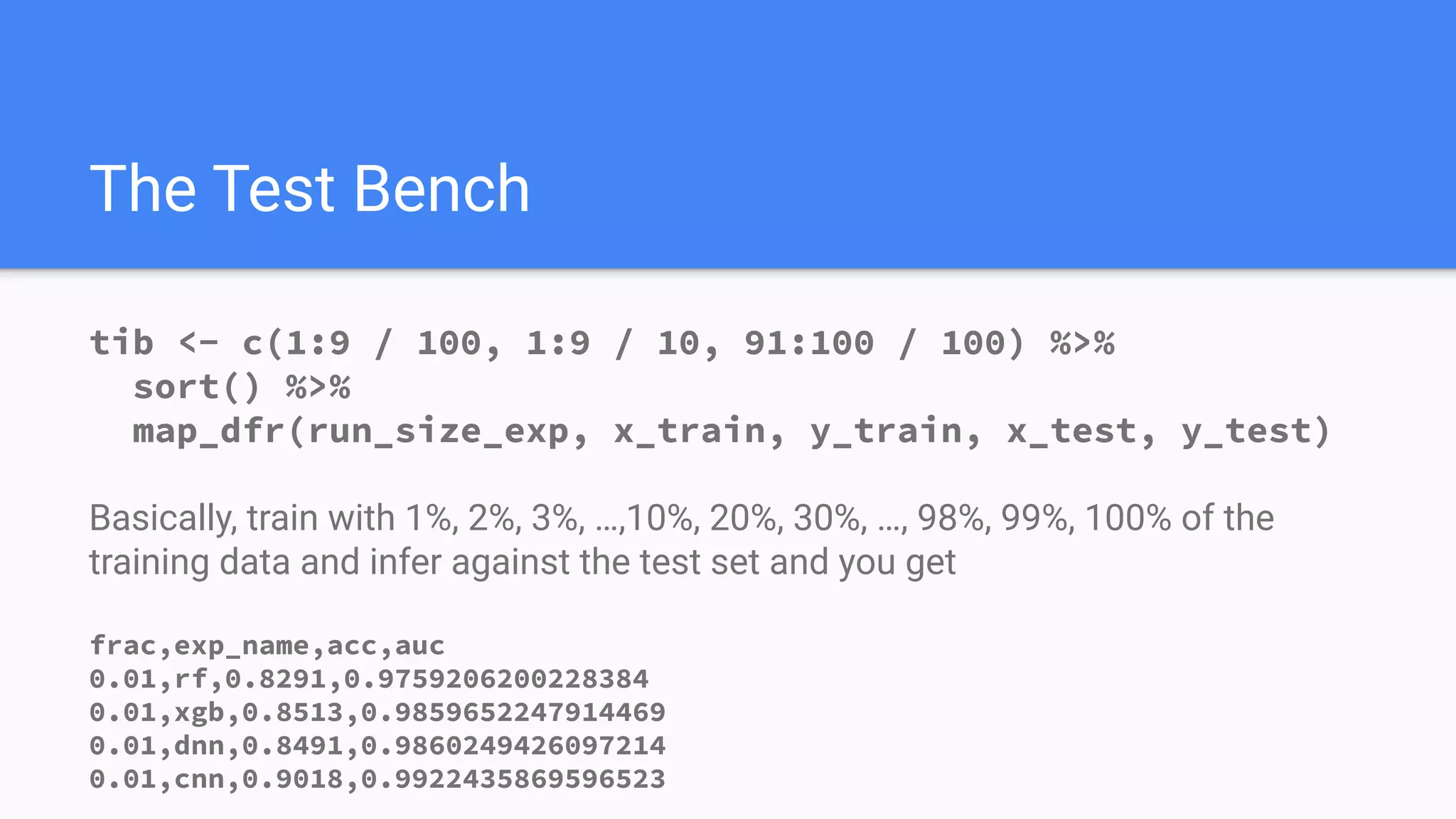
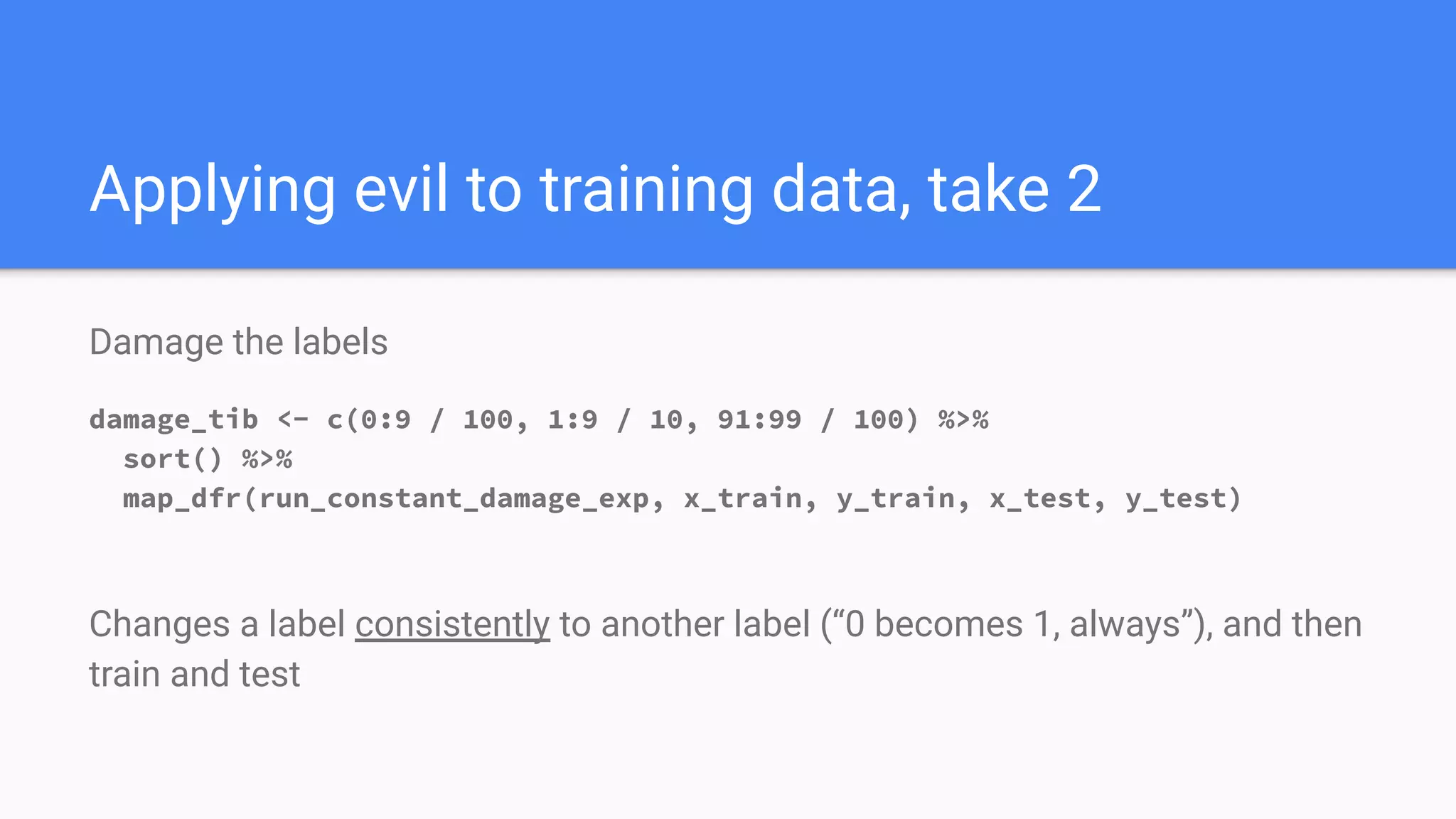
20. run_size_exp
samples <- sample(nrow(x_train), floor(nrow(x_train) * frac), replace=FALSE) - 1
x_t <- x_train[samples,,]
y_t <- y_train[samples]
data <- list(x_train = x_t,
y_train = y_t,
x_test = x_test,
y_test = y_test)
math <- c(rf_exp, xgb_exp, dnn_exp, cnn_exp)
preds <- math %>%
map(exec, !!!data) FIGHT!

21. ML Metrics: Accuracy, AUC
Accuracy: how well the model predicted the true class, compared to predictions
of all other classes.
AUC: Area Under the Curve:
How well the model
is able to separate
classes
Images: https://towardsdatascience.com/understanding-auc-roc-curve-68b2303cc9c5

24. What did we
learn?

25. LHS of the Data
At 1%, we have 60 observations
per class. 2% is 120
observations...
● Adding training data leads
to steep improvement in
response
○ BIGGER DATA!
● Moving to different models
leads to steep
improvements
○ BETTER MATH!

26. RHS of the Data
At 30%, we have 1800
observations per class. 40% is
2400 observations...
● Adding training data leads
to moderate improvement
in response
○ BIGGER DATA!
● Moving to different models
leads to step
improvements
○ BETTER MATH!

27. “Bigger Data
Beats Better
Math, No
Question”
W
HOOPS!

28. If you are already
at the “BEST”
MATH, BIGGER
DATA is a good
strategy
In practice: use whatever works best
on ImageNet…
Andrej Karpathy, CS231N

29. What about
Better Data?

31. What is Better Data?
Training a classifier (“shirt, trouser, handbag, …”) requires training data.
Training a good classifier requires high-confidence in your training data.
Fashion has 60,000 observations for training: 6,000 examples of each class
that we assume are correct to learn from
What if that assumption is not correct?
How can we invalidate the assumption of correctness?

32. That’s right,
expose the data
labels to Pure Evil

33. Teratogenic Effects of Pure Evil in Ursus Teddius Domesticus, Dr. Allison von Lonsdale, Institute for Dangerous Research,
Department of Mad Biology.

34. HIM and Mojo Jojo from the Powerpuff Girls

35. Damage the labels
damage_tib <- c(0:9 / 100, 1:9 / 10, 91:99 / 100) %>%
sort() %>%
map_dfr(run_random_damage_exp, x_train, y_train, x_test, y_test)
Randomly changes a “true” label to one of the other 9, and then train and test
Applying evil to training data

39. But is that really
the most evil we
can be to data?

40. Random Bias
With a random bias, every mis-label has a 1-in-9 chance of being some other
label - the counter-signal is smeared out
Machine Learning needs strong signals to learn and the information content in
the 1-in-9 isn’t relatively strong
Will a constant bias be more damaging?

41. memegenerator.net

42. Damage the labels
damage_tib <- c(0:9 / 100, 1:9 / 10, 91:99 / 100) %>%
sort() %>%
map_dfr(run_constant_damage_exp, x_train, y_train, x_test, y_test)
Changes a label consistently to another label (“0 becomes 1, always”), and then
train and test
Applying evil to training data, take 2

46. But is that really
the most evil we
can be to data?

47. Expose the data to a pack of middle school girls - there are some things I will not do to data

48. What if we ‘fix’
the architecture
and vary samples
and bias?

49. Some test bench code
damage_frac <- c(0:5 / 10) %>%
sort()
sample_frac <- c(1:9/100, 1:9 / 10, 91:100 / 100) %>%
sort()
cross_prod <- cross_df(list(d=damage_frac, s=sample_frac))
results_tib <-
map2_dfr(cross_prod$d, cross_prod$s, run_cnn_damage_exp,
x_train, y_train, x_test, y_test)

51. Observations needed for > 90% accuracy
| quality | acc| frac_sample| num_obs| d_obs|
|--------:|-----:|-----------:|-------:|-----:|
| 1.0| 0.902| 0.40| 24000| NA|
| 0.9| 0.900| 0.50| 30000| 0.25|
| 0.8| 0.904| 0.70| 42000| 0.40|
| 0.7| 0.902| 0.94| 56400| 0.34|

53. Observations needed for > 98% AUC
| quality | auc| frac_sample| num_obs| d_obs|
|--------:|-----:|-----------:|-------:|-----:|
| 1.0| 0.981| 0.05| 3000| NA|
| 0.9| 0.981| 0.10| 6000| 1.0|
| 0.8| 0.981| 0.20| 12000| 1.0|
| 0.7| 0.980| 0.50| 30000| 1.5|

54. An economic argument for quality
∂data size
∂quality
<< -1
One step in quality does not
equal a similarly sized step in
the number of observations
If data is hard to acquire, a
little effort on quality goes a
long way

55. Some thoughts
from the Internet

56. Andrej
Karpathy’s
ML Rubric
In practice: use whatever works best on ImageNet. If you’re feeling a bit
of a fatigue in thinking about the architectural decisions, you’ll be pleased
to know that in 90% or more of applications you should not have to worry
about these. I like to summarize this point as “don’t be a hero”: Instead of
rolling your own architecture for a problem, you should look at whatever
architecture currently works best on ImageNet, download a pretrained
model and finetune it on your data. You should rarely ever have to train a
ConvNet from scratch or design one from scratch.
Andrej Karpathy, CS231N

57. Closing Thoughts
Better Math
● Always worthwhile; research effort, unplannable at the limit
Bigger Data
● Always worthwhile, engineering effort usually
Better Data
● For a given ML metric, ∂data / ∂quality << -1. This implies that overcoming
bias is costly

58. Thanks!
Brent Schneeman
schneeman@gmail.com
brent@alegion.com
@schnee
https://github.com/schnee/big-data-big-math