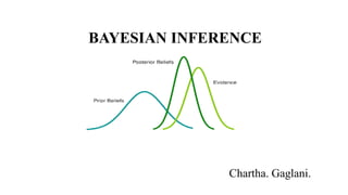
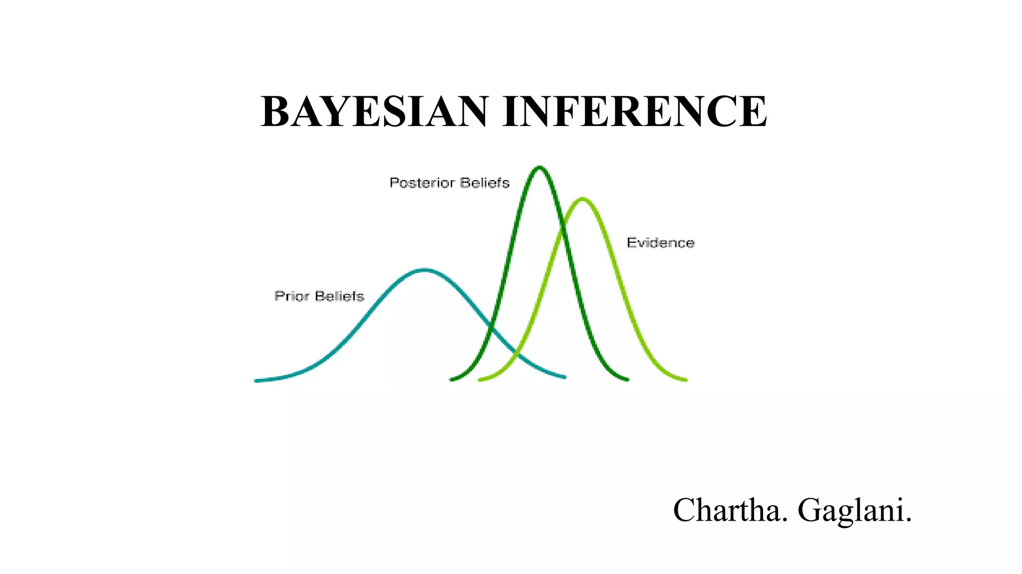
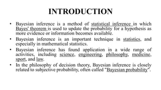
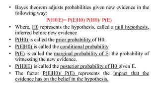
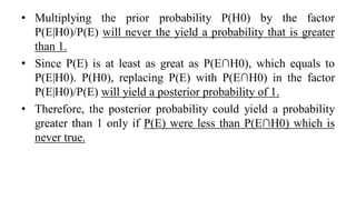
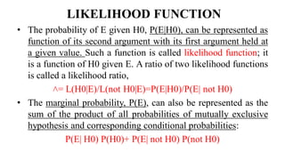
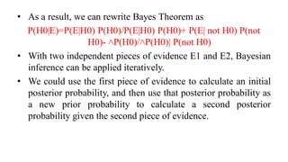
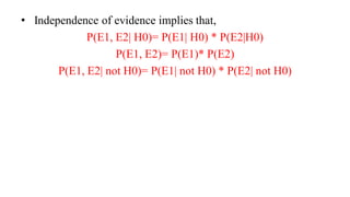
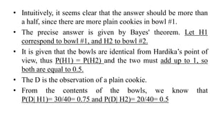
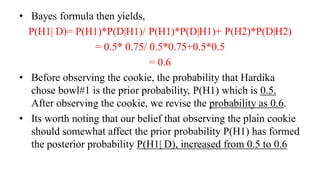
This document provides an overview of Bayesian inference: - Bayesian inference uses Bayes' theorem to update probabilities of hypotheses as new evidence becomes available. It is widely used in science, engineering, medicine and other fields. - Bayes' theorem calculates the posterior probability (probability after seeing evidence) based on the prior probability (initial probability) and the likelihood function (probability of evidence under the hypothesis). 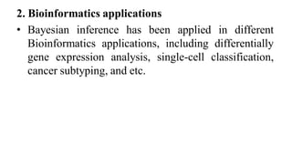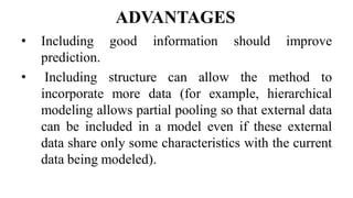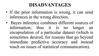- Common applications of Bayesian inference include artificial intelligence, expert systems, bioinformatics, and more. Advantages include incorporating prior information to improve predictions, while disadvantages include potential issues if prior information is incorrect.

1. BAYESIAN INFERENCE
Chartha. Gaglani.

2. CONTENTS
1. Introduction
2. Likelihood function
3. Example
4. Prior probability distribution
5. Introduction to Naïve Bayes
6. Applications
7. Advantages
8. Disadvantages

3. INTRODUCTION
• Bayesian inference is a method of statistical inference in which
Bayes' theorem is used to update the probability for a hypothesis as
more evidence or information becomes available.
• Bayesian inference is an important technique in statistics, and
especially in mathematical statistics.
• Bayesian inference has found application in a wide range of
activities, including science, engineering, philosophy, medicine,
sport, and law.
• In the philosophy of decision theory, Bayesian inference is closely
related to subjective probability, often called "Bayesian probability".

4. • Bayes theorem adjusts probabilities given new evidence in the
following way:
P(H0|E)= P(E|H0) P(H0)/ P(E)
• Where, H0 represents the hypothesis, called a null hypothesis,
inferred before new evidence
• P(H0) is called the prior probability of H0.
• P(E|H0) is called the conditional probability
• P(E) is called the marginal probability of E: the probability of
witnessing the new evidence.
• P(H0|E) is called the posterior probability of H0 given E.
• The factor P(E|H0)/ P(E) represents the impact that the
evidence has on the belief in the hypothesis.

5. • Multiplying the prior probability P(H0) by the factor
P(E|H0)/P(E) will never the yield a probability that is greater
than 1.
• Since P(E) is at least as great as P(E∩H0), which equals to
P(E|H0). P(H0), replacing P(E) with P(E∩H0) in the factor
P(E|H0)/P(E) will yield a posterior probability of 1.
• Therefore, the posterior probability could yield a probability
greater than 1 only if P(E) were less than P(E∩H0) which is
never true.

7. LIKELIHOOD FUNCTION
• The probability of E given H0, P(E|H0), can be represented as
function of its second argument with its first argument held at
a given value. Such a function is called likelihood function; it
is a function of H0 given E. A ratio of two likelihood functions
is called a likelihood ratio,
˄= L(H0|E)/L(not H0|E)=P(E|H0)/P(E| not H0)
• The marginal probability, P(E), can also be represented as the
sum of the product of all probabilities of mutually exclusive
hypothesis and corresponding conditional probabilities:
P(E| H0) P(H0)+ P(E| not H0) P(not H0)

8. • As a result, we can rewrite Bayes Theorem as
P(H0|E)=P(E|H0) P(H0)/P(E|H0) P(H0)+ P(E| not H0) P(not
H0)- ˄P(H0)/˄P(H0)| P(not H0)
• With two independent pieces of evidence E1 and E2, Bayesian
inference can be applied iteratively.
• We could use the first piece of evidence to calculate an initial
posterior probability, and then use that posterior probability as
a new prior probability to calculate a second posterior
probability given the second piece of evidence.

9. • Independence of evidence implies that,
P(E1, E2| H0)= P(E1| H0) * P(E2|H0)
P(E1, E2)= P(E1)* P(E2)
P(E1, E2| not H0)= P(E1| not H0) * P(E2| not H0)

10. From which bowl is the cookie?
• Suppose there are two full bowls of cookies. Bowl #1 has 10
chocolate chip and 30 plain cookies, while bowl #2 has 20 of each.
Our friend Hardika picks a bowl at random, and then picks a cookie
at random. We may assume there is no reason to believe Hardika
treats one bowl differently from another, likewise for the cookies.
The cookie turns out to be a plain one. How probable is it that
Hardika picked it out of bowl #1?
Bowl#1 Bowl#2

11. • Intuitively, it seems clear that the answer should be more than
a half, since there are more plain cookies in bowl #1.
• The precise answer is given by Bayes' theorem. Let H1
correspond to bowl #1, and H2 to bowl #2.
• It is given that the bowls are identical from Hardika’s point of
view, thus P(H1) = P(H2) and the two must add up to 1, so
both are equal to 0.5.
• The D is the observation of a plain cookie.
• From the contents of the bowls, we know that
P(D| H1)= 30/40= 0.75 and P(D| H2)= 20/40= 0.5

12. • Bayes formula then yields,
P(H1| D)= P(H1)*P(D|H1)/ P(H1)*P(D|H1)+ P(H2)*P(D|H2)
= 0.5* 0.75/ 0.5*0.75+0.5*0.5
= 0.6
• Before observing the cookie, the probability that Hardika
chose bowl#1 is the prior probability, P(H1) which is 0.5.
After observing the cookie, we revise the probability as 0.6.
• Its worth noting that our belief that observing the plain cookie
should somewhat affect the prior probability P(H1) has formed
the posterior probability P(H1| D), increased from 0.5 to 0.6

13. • This reflects our intuition that the cookie is more likely from
the bowl#1, since it has a higher ratio of plain to chocolate
cookies than the other.

14. PRIOR PROBABILITY DISTRIBUTION
• In Bayesian statistical inference, a prior probability
distribution, often called simply the prior, of an uncertain
quantity p( For e.g. suppose p is the proportion of voters who
will vote for Mr. Narendra Modi in a future election) is the
probability distribution that would express ones uncertainty
about p before the data (For e.g. an election poll) are taken into
account.
• It is meant to attribute uncertainty rather than randomness to
the uncertain quantity.

15. INTRODUCTION TO NAIVE BAYES
• Suppose your data consist of fruits, described by their color
and shape.
• Bayesian classifiers operate by saying “If you see a fruit that is
red and round, which type of fruit most likely to be, based on
the observed data sample? In future, classify red and round
fruit as that type of fruit.”
• A difficulty arises when you have more than a few variables
and classes- you would require an enormous number of
observations to estimate these probabilities.

16. • Naïve Bayes classifier assume that the effect of a variable
value on a given class is independent of the values of other
variable.
• This assumption is called class conditional independence.
• It is made to simplify the computation and in this sense
considered to be Naïve.

17. APPLICATIONS
1. Computer applications
• Bayesian inference has applications in artificial
intelligence and expert systems.
• Bayesian inference techniques have been a fundamental
part of computerized pattern recognition techniques since
the late 1950s.
• Recently Bayesian inference has gained popularity among
the phylogenetics community for these reasons; a number
of applications allow many demographic and evolutionary
parameters to be estimated simultaneously.

19. 2. Bioinformatics applications
• Bayesian inference has been applied in different
Bioinformatics applications, including differentially
gene expression analysis, single-cell classification,
cancer subtyping, and etc.

20. ADVANTAGES
• Including good information should improve
prediction.
• Including structure can allow the method to
incorporate more data (for example, hierarchical
modeling allows partial pooling so that external data
can be included in a model even if these external
data share only some characteristics with the current
data being modeled).

21. DISADVANTAGES
• If the prior information is wrong, it can send
inferences in the wrong direction.
• Bayes inference combines different sources of
information; thus it is no longer an
encapsulation of a particular dataset (which is
sometimes desired, for reasons that go beyond
immediate predictive accuracy and instead
touch on issues of statistical communication).

22. THANK YOU.