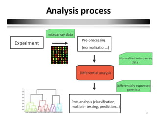
This document summarizes a study that compares 8 different statistical tests for differential gene expression analysis on microarray data. The study uses simulations with different data models to evaluate the power and performance of each test under various conditions. The tests are applied to the simulated data to identify differentially expressed genes and their ability to correctly detect differentially expressed genes is assessed and compared across the different simulation models.

1. Should we abandon the t-test ?
A statistical comparison of 8 differential gene expression tests
Marine Jeanmougin, Master student INSA-Lyon
Mickaël Guedj1,3, Grégory Nuel2,3
SMPGD’09
1. Ligue Nationale contre le Cancer – Cartes d’Identité des Tumeurs program (CIT)
2. Paris Descartes University – MAP5 laboratory
3. Statistics for Systems Biology working group

2. Analysis process
microarray data
Pre-processing
Experiment
(normalization…)
Normalized microarray
data
Differential analysis
Differentially expressed
gene lists
Post-analysis (classification,
multiple- testing, prediction…)
2

3. Hypothesis testing
Differential analysis : comparison of 2 populations (or more)
according to a variable of interest (expression level).
Statistical hypothesis : assumption about a population parameter :
2 types of statistical hypotheses :
H0 : Expression level is the same between the 2 populations
H1 : Expression level differs between the 2 populations
3

4. Power
H0 accepted H0 rejected
H0 TRUE False positif
True negatif
(type I error)
H0 FALSE False negatif
True positif
(type II error)
Type I error rate : α (0.05) Ability of a test to detect a gene as
Powerα = 1 – β differentially expressed, given that
Type II error rate : β this gene is actually differentially
expressed.
Compare power according to a same type I error rate 4

5. In literature
Numerous tests dedicated to the differential analysis :
Performs differently according to :
• Sample size
• Data noise
• Distribution of expression levels
Various conditions of application
A lack of comparison studies in the literature (Jeffery et al. 2006)
Choosing one test is difficult
5

6. Variance modelling
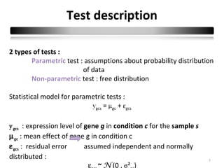
An essential point: variance modelling
«…accurate estimation of variability is difficult. » (RVM, Wright and Simon, 2003)
« The importance of variance modelling is now widely known…» (SMVar, Jaffrézic et al, 2007)
« Many different sources of variability affect gene expression intensity measurements […]. Not at
all are well characterized or even identified» (VarMixt, Delmar et al, 2004)
Many approaches :
6

7. Test description
2 types of tests :
Parametric test : assumptions about probability distribution
of data
Non-parametric test : free distribution
Statistical model for parametric tests :
ygcs = µgc + εgcs
y gcs : expression level of gene g in condition c for the sample s
µ gc : mean effect of gene g in condition c
ε gcs : residual error assumed independent and normally
distributed : 7
ε ~ N (0 , σ² )

8. Test Variance modeling Reference Package R
- Fixed variance
Welch’s T-test - Heterodasticity Welch CIT (internal)
- Fixed variance
ANOVA - homoscedasticity Fisher CIT (internal)
Wilcoxon Non parametric Wilcoxon stats
Tusher et al
SAM Non parametric
2001
samr
Inverse gamma distribution on the Wright & Simon
RVM variance (estimated from all the data set) 2003
CIT (internal)
Moderate t-test. Usual variance replaced
Smyth
Limma by a conditional variance. Bayesian
2004
limma
approach
Delmar et al
VARMIXT Gamma mixture model on the variance
2005
varmixt
Mixed model (fixed condition effect and Jaffrézic et al
SMVAR random gene effect) 2007
SMVar
8

9. Comparison process
9

10. Simulations
Parameters (determined with CIT datasets):
• sample size
• genes number
• µ: mean of expression level
• σ: standard deviation
• π0 and π1: proportions of genes under H0 and H1
samples
Simulated under
H0
genes
Simulated under
H1
group A group B
Assumption: independence of genes 10

11. Simulations
Model 1: Gaussian model Model 2: Uniform model
Ygcs ~ N (µobs , σ²obs) Ygcs ~ U (a,b)
H0: µA = µB
H0: µA = µB H1: µB = µA + dm
H1: µB = µA + dm
Model 3: Mixture model on variances Model 4: Small variances model
Ygcs ~ N (µobs , σ²group *) Ygcs ~ N (µobs , σ²gv *)
H0: µA = µB H0: µA = µB
H1: µB = µA + dm H1: µB = µA + dm
* Groups of variance are simulated * 1000 genes (10%) are simulated with
a small variance and small expression
level 11

12. Simulations
Model 1: Gaussian model Model 2: Uniform model
Ygcs ~ N (µ , σ²obs) Ygcs ~ U (a,b)
H0: µA = µB
H0: µA = µB H1: µB = µA + dm
H1: µB = µA + dm
Model 3: Mixture on variances model Model 4: Small variances model
Ygcs ~ N (µ , σ²group *) Ygcs ~ N (µ , σ²gv *)
H0: µA = µB H0: µA = µB
H1: µB = µA + dm H1: µB = µA + dm
* Groups of variance are simulated * 1000 genes (10%) are simulated with
a small variance and small expression
level 12

13. Simulations
Model 1: Gaussian model Model 2: Uniform model
Ygcs ~ N (µ , σ²obs) Ygcs ~ U (a,b)
H0: µA = µB
H0: µA = µB H1: µB = µA + dm
H1: µB = µA + dm
Model 3: Mixture on variances model Model 4: Small variances model
Ygcs ~ N (µ , σ²group *) Ygcs ~ N (µ , σ²gv *)
H0: µA = µB H0: µA = µB
H1: µB = µA + dm H1: µB = µA + dm
* Groups of variance are simulated * 1000 genes (10%) are simulated with
a small variance and small expression
level 13

14. Simulations
Model 1: Gaussian model Model 2: Uniform model
Ygcs ~ N (µ , σ²obs) Ygcs ~ U (a,b)
H0: µA = µB
H0: µA = µB H1: µB = µA + dm
H1: µB = µA + dm
Model 3: Mixture on variances model Model 4: Small variances model
Ygcs ~ N (µ , σ²group *) Ygcs ~ N (µ , σ²gv *)
H0: µA = µB H0: µA = µB
H1: µB = µA + dm H1: µB = µA + dm
* Groups of variance are simulated * 1000 genes (10%) are simulated with
a small variance and small expression
level 14

15. Simulations
Model 1: Gaussian model Model 2: Uniform model
Ygcs ~ N (µ , σ²obs) Ygcs ~ U (a,b)
H0: µA = µB
H0: µA = µB H1: µB = µA + dm
H1: µB = µA + dm
Model 3: Mixture on variances model Model 4: Small variances model
Ygcs ~ N (µ , σ²group *) Ygcs ~ N (µ , σ²gv *)
H0: µA = µB H0: µA = µB
H1: µB = µA + dm H1: µB = µA + dm
* Groups of variance are simulated * 1000 genes (10%) are simulated with
a small variance and small expression
level 15

16. Simulations
Model 4 :
H0
Gene with small
variances H1
group A group B
16

17. Results : 1 model (gaussian)
st
1 – Power according to sample size

18. Results : 1 model (gaussian)
st
1 – Power according to sample size

19. Results : 1 model (gaussian)
st
Small sample Large sample
Tests sizes sizes
1 – Power according to sample size n=10 n=200
T-test - =
3.83-4.61 4.92-5.8
Anova = =
4.46-5.24 4.92-5.8
Wilcoxo - +
n 2.78-3.46 5.14-6.04
= =
SAM
4.59-5.45 4.96-5.84
+ +
RVM
5.74-6.68 5.01-5.89
= =
Limma
4.64-5.5 4.98-5.86
+ +
SMVar
7.04-8.08 5.08-5.98
= =
VarMixt
4.65-5.51 4.99-5.87

20. Results : 1 model (gaussian)
st
1 – Power according to sample size
Adjusted Type I error rate

21. Results : 1st model (gaussian)
1 – Power relative to t-test, according to sample size
Loss of power Gain in power
t-test 21

22. Results : 1st model (gaussian)
1 – Power according to difference mean (dm)
Adjusted Type I error rate
Loss Gain Loss Gain
t-test t-test
Same observations

23. Results : 1st model (gaussian)
Conclusions :
Few power differences
Observed differences in small sample sizes partly due to
type I error rates
Wilcoxon: less powerful
Limma and varmixt : similar good results
Anova : equivalent to the t-test

24. Results : 2nd model (uniform)
1 – Power according to sample size
Adjusted Type I error rate
Loss Gain Loss Gain
t-test t-test
SMVar didn’t converge for this simulation model

25. Results
Conclusions model 2 (uniform):
Results are similar to the first 1st model
Wilcoxon : no improvement
unexpected
T-test : no loss of power
results are robust to the assumption of Gaussian distribution
Conclusion models 3 (groups of variance) and 4 (small
variances):
Similar results

26. Random test:
Reference test. 10 000 p-values are sampled from an uniform distribution U(0,1).
26

27. Gene lists
Sample
Project Condition Genes Publication
sizes
Disease staging Lamant et
lymphoid tumors 22 283 37
Gender al, 2007
TP53 mutation Boyault et
Liver tumors 22 283 65
Gender al, 2006
Rickman et
head and neck tumors Gender 22 283 81
al, 2008
Soulier et al,
leukemia Gender 22 283 104
2006
Bertheau et
Response to treatment
breast tumors 22 283 500 al, 2007
ESR1
27

28. Gene lists
for each
dataset 5
datasets
FDR: 0.05, 0.1, 0.3,0.5
Sample size: complete dataset, 10, 20
dendrograms
g3 0 1011... binary metric
g72 1 Ward’s method
g110 0
9 gene lists . 0
(8 tests + “rand”) . 1
. .
. Principal
. PCA Component
Analysis
Count
Rand: Random Test (sample 10 000 p-values from an matrix
uniform distribution)
FDR: False discovery rate (Benjamini and Hochberg) 28

29. Gene lists : results
lymphoid tumors / disease staging
leukemia / gender
FDR = 0.05
Complete
dataset
breast tumors /
response to treatment

30. Gene lists : results
lymphoid tumors / disease staging
leukemia / gender
FDR = 0.05
Complete
dataset
T-test
SMVar
Wilcoxon
breast tumors /
response to treatment

31. Gene lists : results
FDR = 0.05
Complete
dataset
breast tumors / ESR1 lymphoid tumors / gender
RVM
Limma
Anova head and neck
Varmixt tumors / gender

32. Gene lists : results (PCA)
FDR = 0.05
Complete
dataset
RVM T-test
Limma SMVar
leukemia/gender Anova Wilcoxon
Varmixt SAM
breast tumors/response

33. Spike-in dataset
Human Genome U133 dataset:

34. Spike-in dataset : results
Type I error rates :
T-test Anova Wilcoxon SAM RVM Limma SMVar Varmixt
Type I error
rates - = - = + = + =
same results as simulations

35. Spike-in dataset : results
Power according to 13 pairwise comparisons
Adjusted Type I error rate
Loss Gain Loss Gain

36. Re-sampling approach
Differentially Expressed Genes
(pv < 1.10-4)
Breast tumor
500 samples
Non-Differentially Expressed Genes
(pv > 0.1)
Sampling
Reduced dataset
(5-5)
X 1000 8 tests + « rand* »
*rand: Random Test (10 000 p-values sampled from a uniform distribution)
Power computation

37. Re-sampling approach: results
37

38. Computation time
Computation time (sec)*
TEST 22 283 genes / 20 samples 52 188 genes / 200 samples
T-test 0.87 5.34
rvm 121.69 585.00
anova 0.91 2.98
Limma 0.95 6.81
Wilcoxon 19.18 107.40
SAM 24.48 415.20
SMVar 0.97 19.72
VarMixt 508.98 1h20
* Intel® Core ™ 2 DUO CPU 38

39. Summary
Comparison according to 3 criterion families :

40. Summary table
Use
40

41. Summary table
Use
41

42. Summary table
Use
42
42

43. Summary table
Use
43
43

44. Conclusions
• We propose a comparison process
• Type I error rates is an issue that explains some differences in power
• Tests cluster: similar gene lists (T-test-SMVar/Varmixt-limma-anova-RVM)
44

45. Conclusions
• We propose a comparison process
• Type I error rates is an issue that explains some differences in power
• Tests cluster: similar gene lists (T-test-SMVar/Varmixt-limma-anova-RVM)
• On large sample sizes: the 8 tests are equivalent
• On small sample sizes: - weak differences in simulations
- more important differences in applications
45

46. Conclusions
• We propose a comparison process
• Type I error rates is an issue that explains some differences in power
• Tests cluster: similar gene lists (T-test-SMVar/Varmixt-limma-anova-RVM)
• On large sample sizes: the 8 tests are equivalent
• On small sample sizes: - weak differences in simulations
- more important differences in applications
• 2 tests inadvisable: Wilcoxon (worse) and SAM (unstable power) => NP tests
• 2 tests appear more efficient: Limma and VarMixt
• Considering an intensive use: Limma
46

47. Thanks
To the whole CIT’s team of the Ligue Nationale Contre le Cancer :
To M. Guedj, L. Marisa, AS. Valin, F. Petel, E. Thomas, R. Schiappa,
L. Vescovo, A. de Reynies, J. Metral and J. Godet
To G. Nuel, MAP5 laboratory, UMR 8145, Paris V University
and V. Dumeaux, Tromsø University et Paris V University
To the IRISA of Rennes
To the SMPGD’s team who enables me to introduce my work

48. Thank you for your attention !
Contact : marine.jeanmougin@gmail.com
48