Asymptotic notations for desing analysis of algorithm.pptx
1.
Comp 122, Spring2004
March 19, 2025
Asymptotic Notation,
Review of Functions &
Summations
2.
ymp - 2Comp 122
Asymptotic Complexity
Running time of an algorithm as a function of
input size n for large n.
Expressed using only the highest-order term in
the expression for the exact running time.
Instead of exact running time, say Q(n2
).
Describes behavior of function in the limit.
Written using Asymptotic Notation.
3.
ymp - 3Comp 122
Asymptotic Notation
Q, O, W, o, w
Defined for functions over the natural numbers.
Ex: f(n) = Q(n2
).
Describes how f(n) grows in comparison to n2
.
Define a set of functions; in practice used to compare
two function sizes.
The notations describe different rate-of-growth
relations between the defining function and the
defined set of functions.
4.
ymp - 4Comp 122
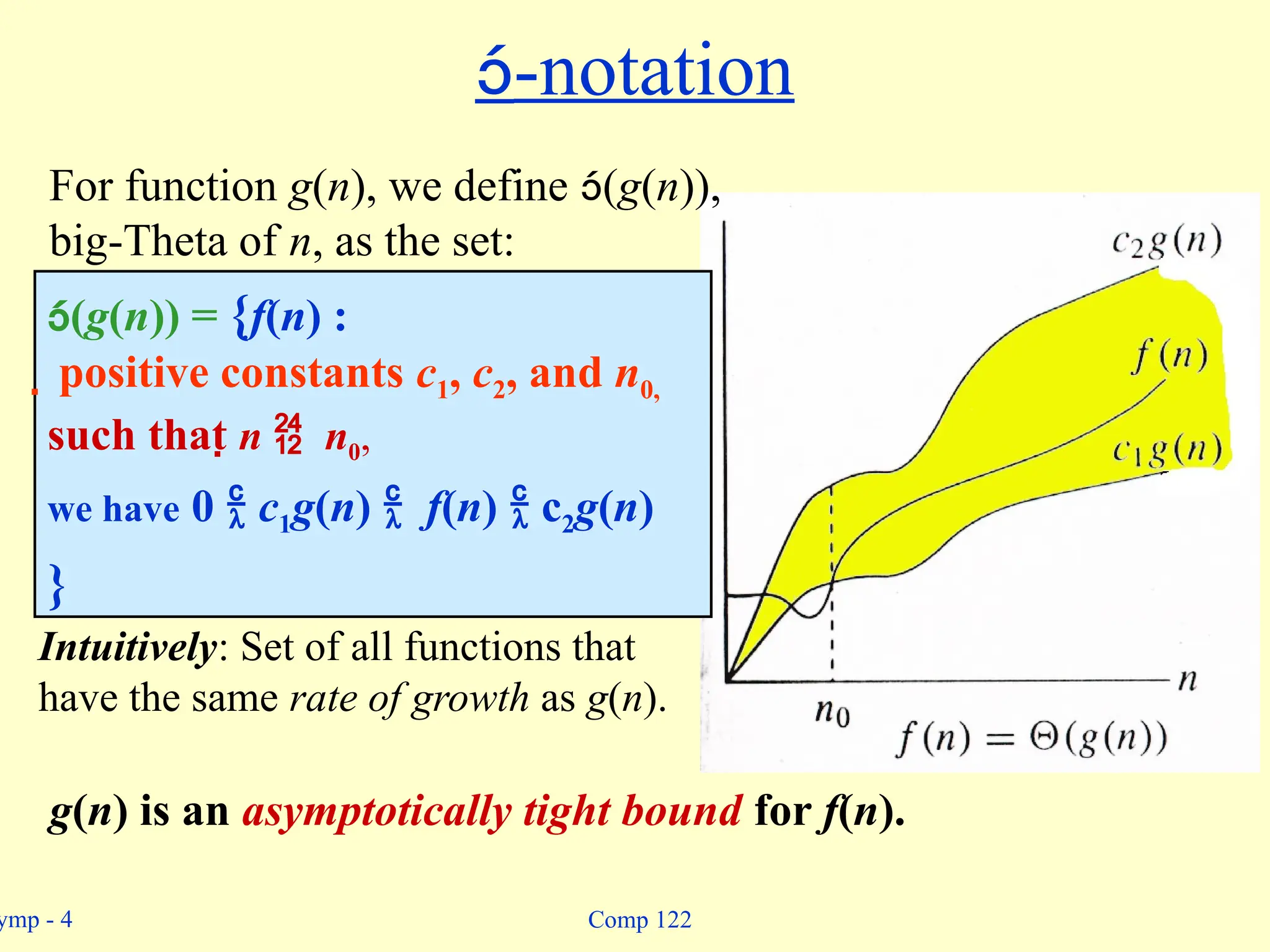
-notation
(g(n)) = {f(n) :
positive constants c1, c2, and n0,
such that n n0,
we have 0 c1g(n) f(n) c2g(n)
}
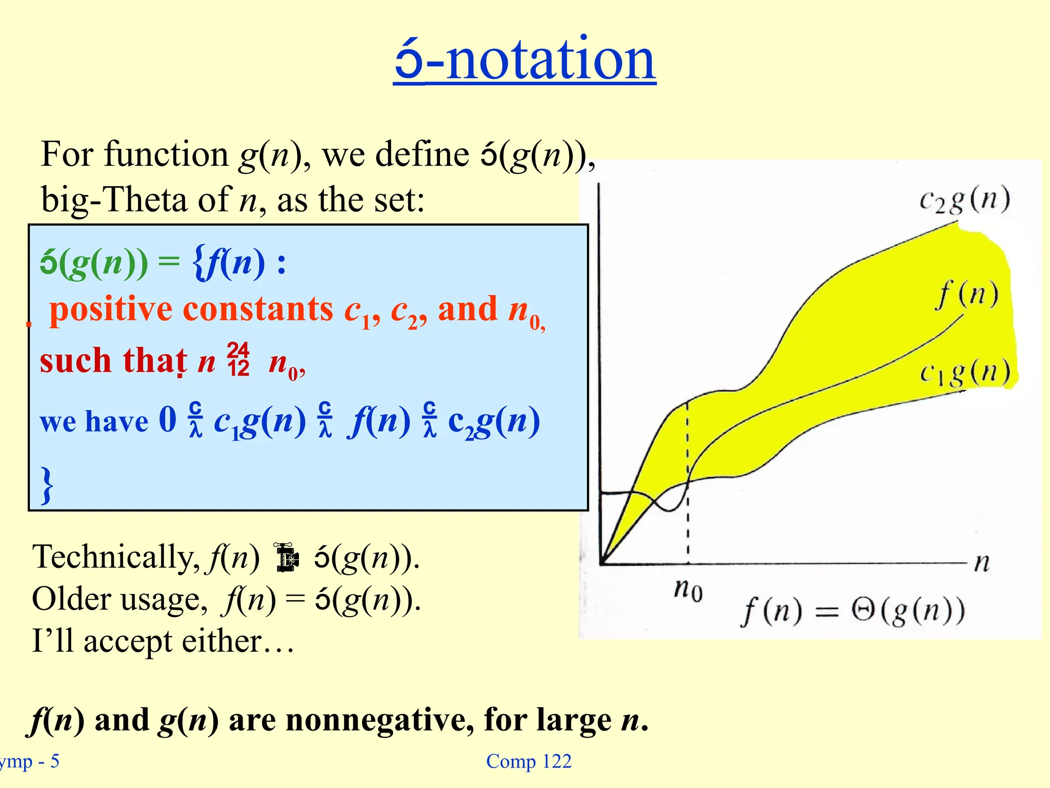
For function g(n), we define (g(n)),
big-Theta of n, as the set:
g(n) is an asymptotically tight bound for f(n).
Intuitively: Set of all functions that
have the same rate of growth as g(n).
5.
ymp - 5Comp 122
-notation
(g(n)) = {f(n) :
positive constants c1, c2, and n0,
such that n n0,
we have 0 c1g(n) f(n) c2g(n)
}
For function g(n), we define (g(n)),
big-Theta of n, as the set:
Technically, f(n) (g(n)).
Older usage, f(n) = (g(n)).
I’ll accept either…
f(n) and g(n) are nonnegative, for large n.
6.
ymp - 6Comp 122
Example
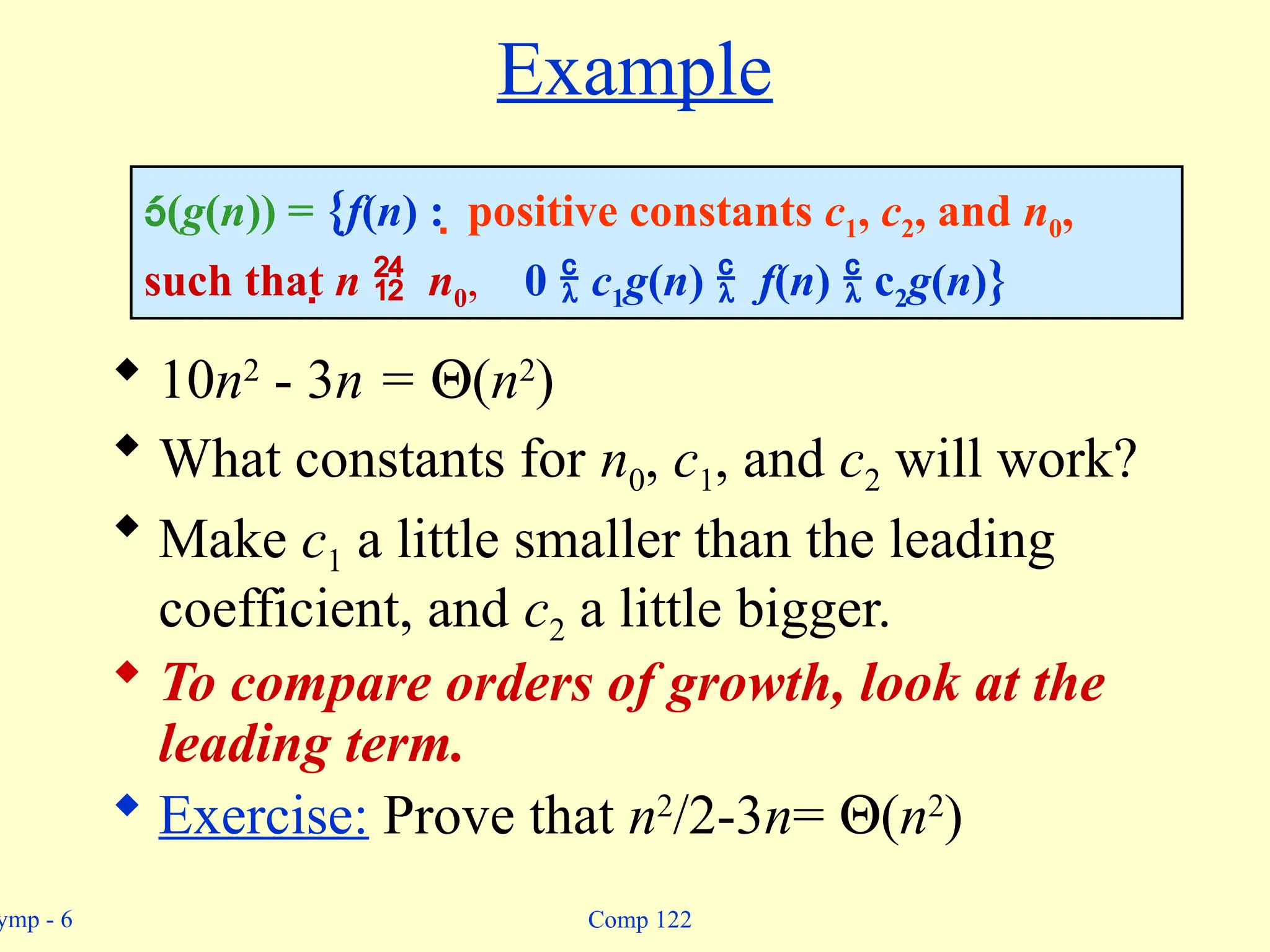
10n2
- 3n = Q(n2
)
What constants for n0, c1, and c2 will work?
Make c1 a little smaller than the leading
coefficient, and c2 a little bigger.
To compare orders of growth, look at the
leading term.
Exercise: Prove that n2
/2-3n= Q(n2
)
(g(n)) = {f(n) : positive constants c1, c2, and n0,
such that n n0, 0 c1g(n) f(n) c2g(n)}
7.
ymp - 7Comp 122
Example
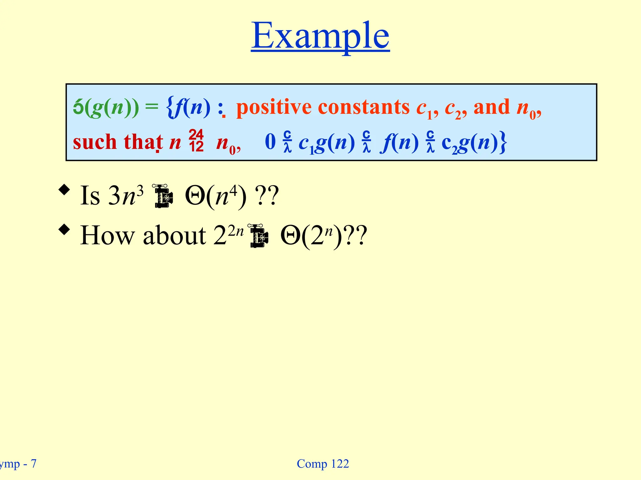
Is 3n3
Q(n4
) ??
How about 22n
Q(2n
)??
(g(n)) = {f(n) : positive constants c1, c2, and n0,
such that n n0, 0 c1g(n) f(n) c2g(n)}
8.
ymp - 8Comp 122
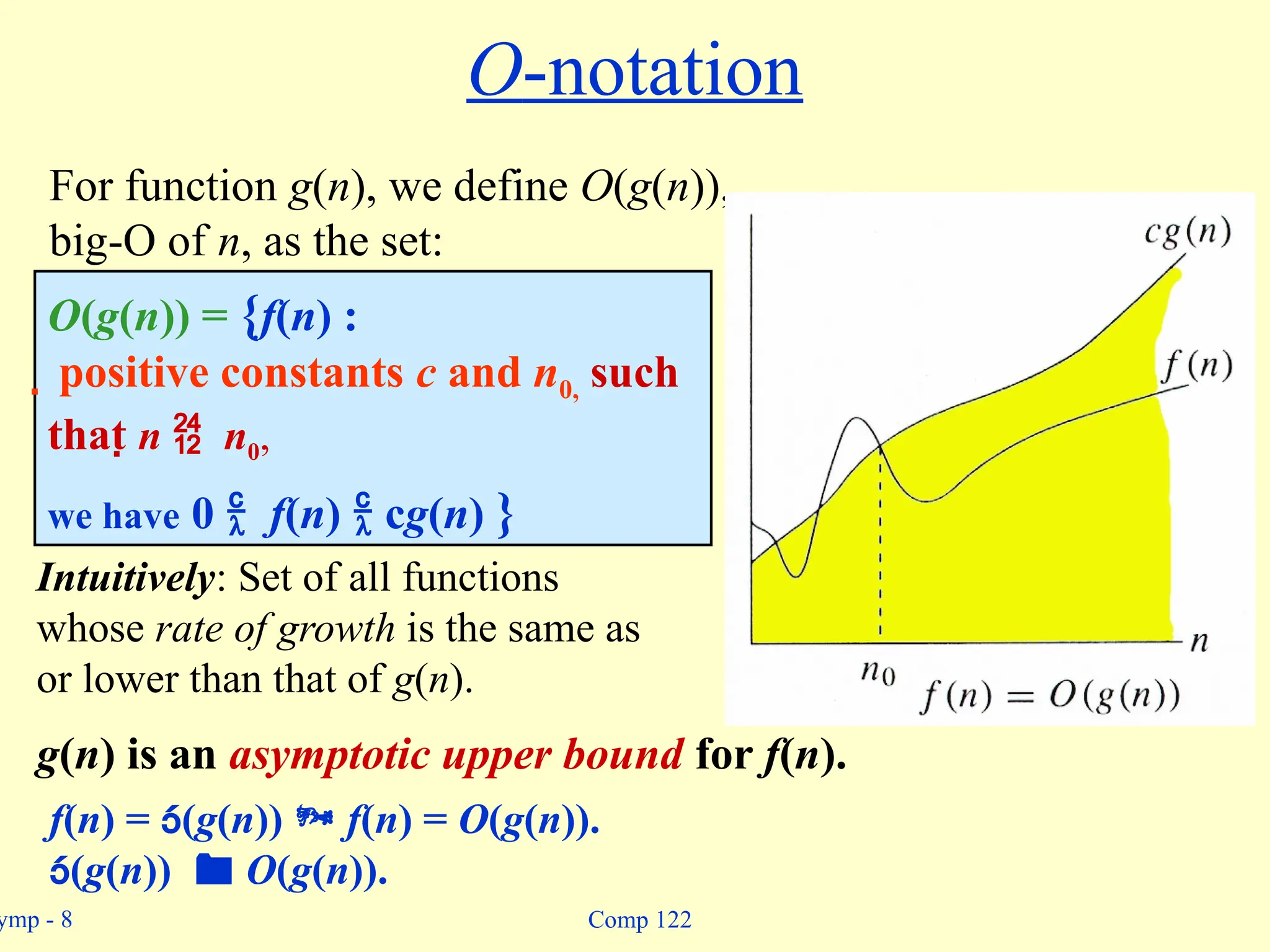
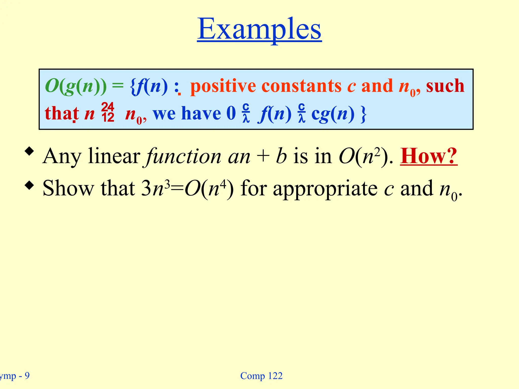
O-notation
O(g(n)) = {f(n) :
positive constants c and n0, such
that n n0,
we have 0 f(n) cg(n) }
For function g(n), we define O(g(n)),
big-O of n, as the set:
g(n) is an asymptotic upper bound for f(n).
Intuitively: Set of all functions
whose rate of growth is the same as
or lower than that of g(n).
f(n) = (g(n)) f(n) = O(g(n)).
(g(n)) O(g(n)).
9.
ymp - 9Comp 122
Examples
Any linear function an + b is in O(n2
). How?
Show that 3n3
=O(n4
) for appropriate c and n0.
O(g(n)) = {f(n) : positive constants c and n0, such
that n n0, we have 0 f(n) cg(n) }
10.
ymp - 10Comp 122
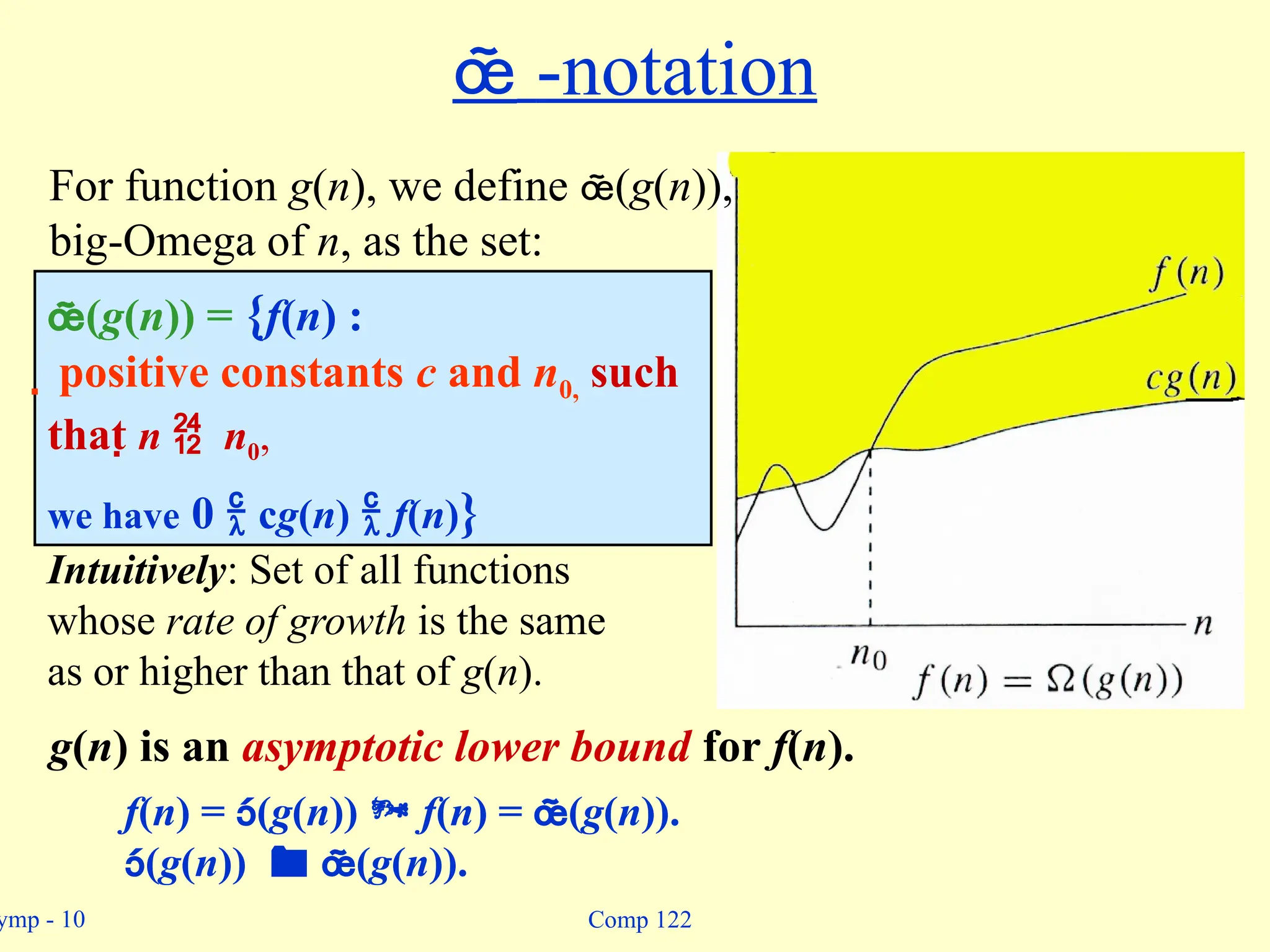
-notation
g(n) is an asymptotic lower bound for f(n).
Intuitively: Set of all functions
whose rate of growth is the same
as or higher than that of g(n).
f(n) = (g(n)) f(n) = (g(n)).
(g(n)) (g(n)).
(g(n)) = {f(n) :
positive constants c and n0, such
that n n0,
we have 0 cg(n) f(n)}
For function g(n), we define (g(n)),
big-Omega of n, as the set:
11.
ymp - 11Comp 122
Example
n = (lg n). Choose c and n0.
(g(n)) = {f(n) : positive constants c and n0, such that
n n0, we have 0 cg(n) f(n)}
ymp - 13Comp 122
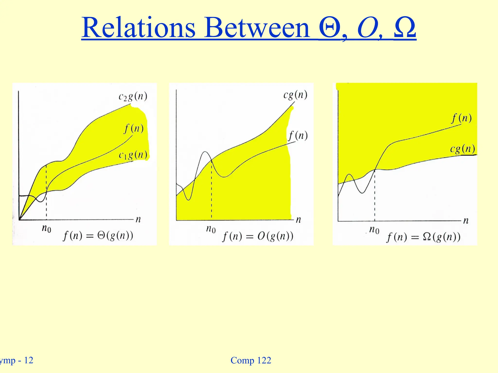
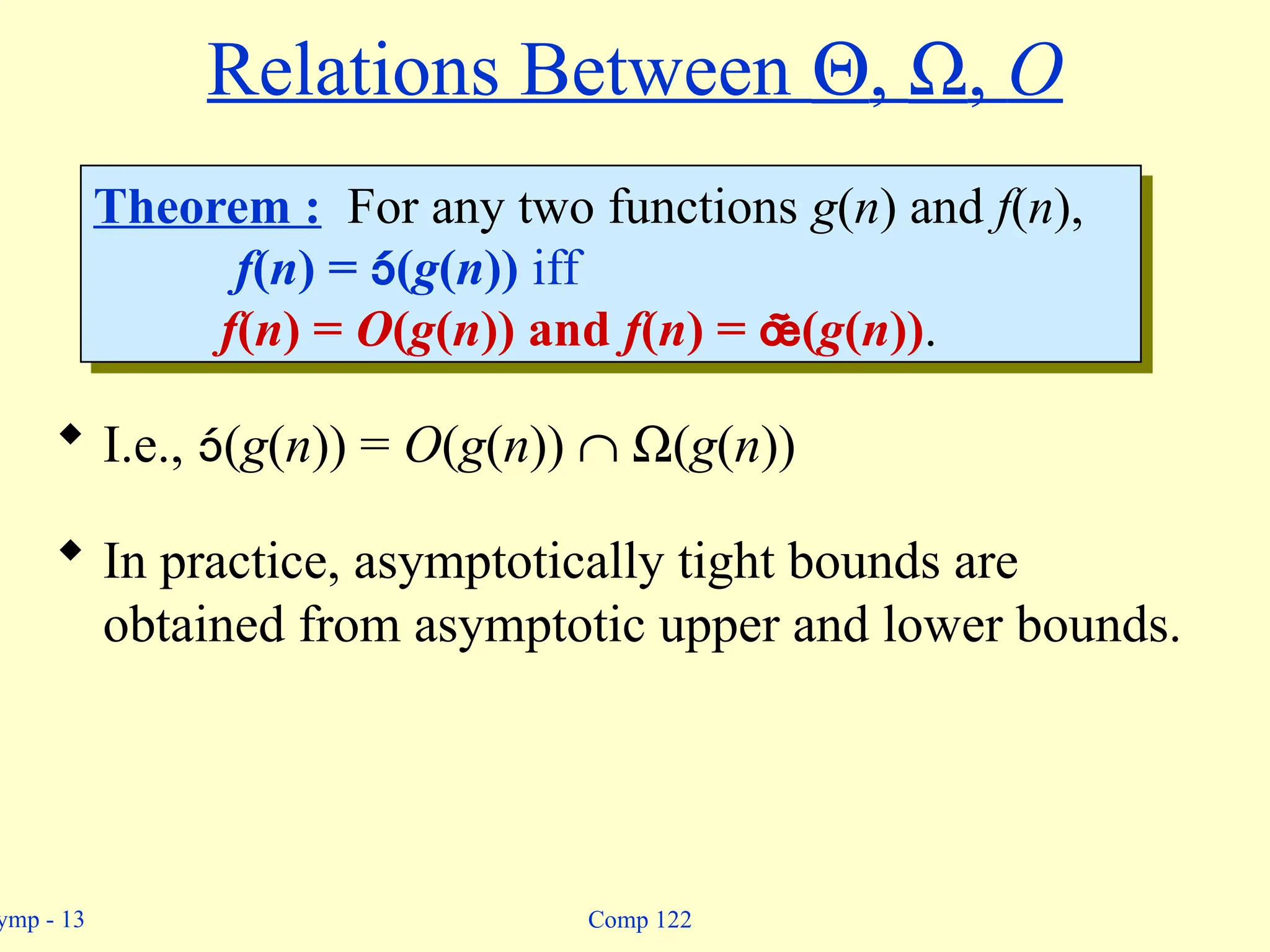
Relations Between Q, W, O
I.e., (g(n)) = O(g(n)) Ç W(g(n))
In practice, asymptotically tight bounds are
obtained from asymptotic upper and lower bounds.
Theorem : For any two functions g(n) and f(n),
f(n) = (g(n)) iff
f(n) = O(g(n)) and f(n) = (g(n)).
14.
ymp - 14Comp 122
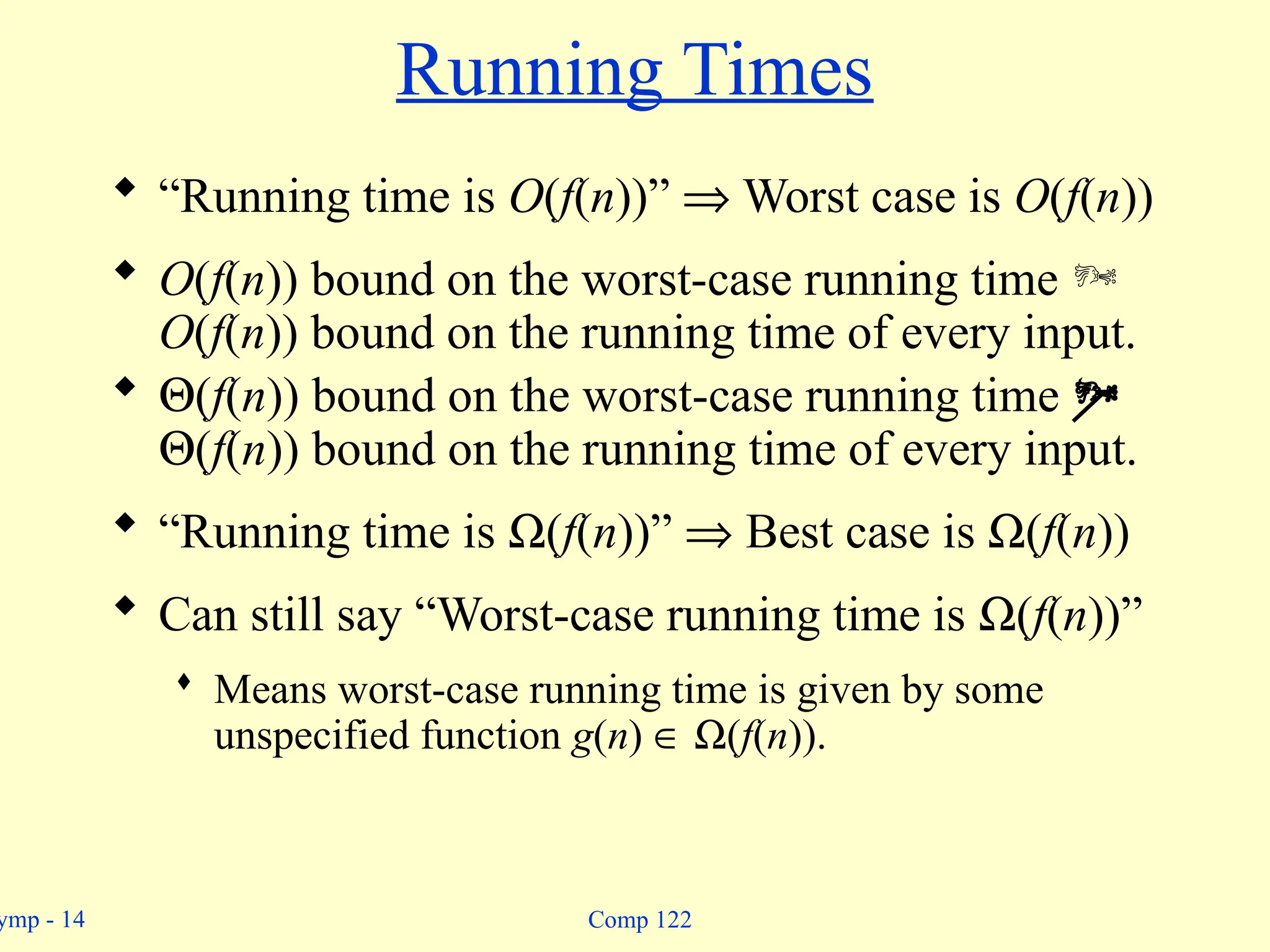
Running Times
“Running time is O(f(n))” Þ Worst case is O(f(n))
O(f(n)) bound on the worst-case running time
O(f(n)) bound on the running time of every input.
Q(f(n)) bound on the worst-case running time
Q(f(n)) bound on the running time of every input.
“Running time is W(f(n))” Þ Best case is W(f(n))
Can still say “Worst-case running time is W(f(n))”
Means worst-case running time is given by some
unspecified function g(n) Î W(f(n)).
15.
ymp - 15Comp 122
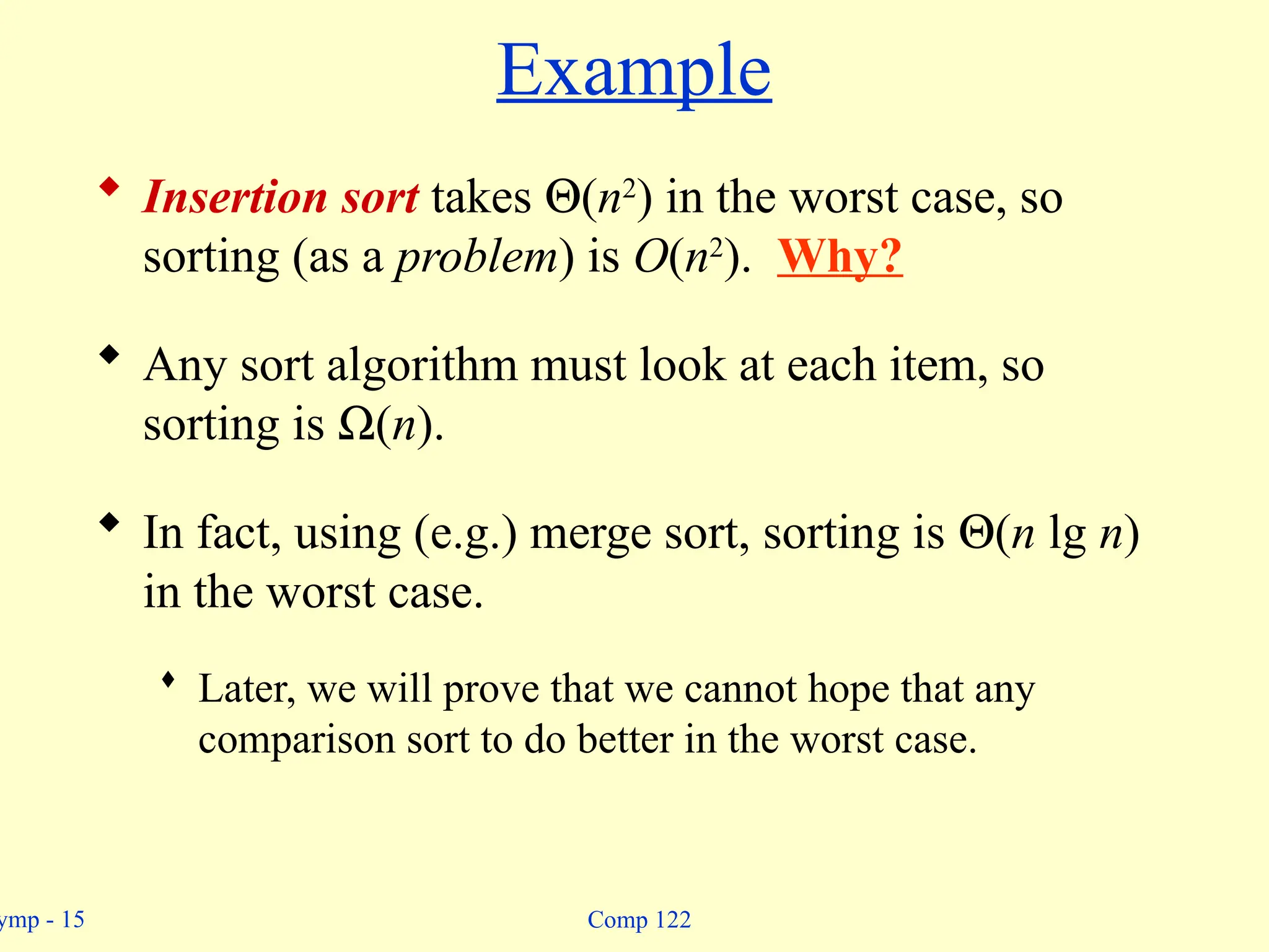
Example
Insertion sort takes Q(n2
) in the worst case, so
sorting (as a problem) is O(n2
). Why?
Any sort algorithm must look at each item, so
sorting is W(n).
In fact, using (e.g.) merge sort, sorting is Q(n lg n)
in the worst case.
Later, we will prove that we cannot hope that any
comparison sort to do better in the worst case.
16.
ymp - 16Comp 122
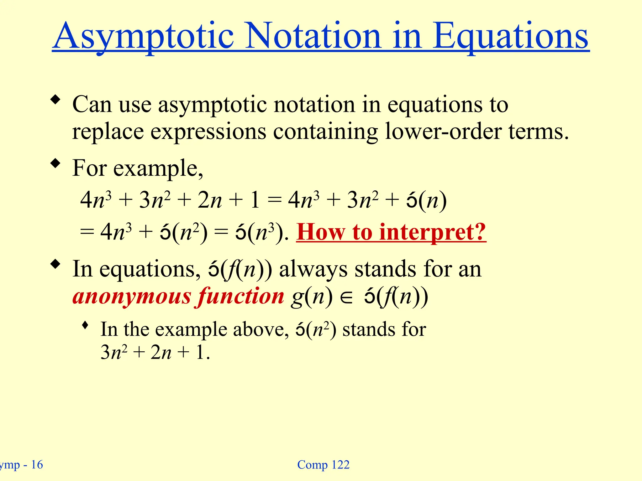
Asymptotic Notation in Equations
Can use asymptotic notation in equations to
replace expressions containing lower-order terms.
For example,
4n3
+ 3n2
+ 2n + 1 = 4n3
+ 3n2
+ (n)
= 4n3
+ (n2
) = (n3
). How to interpret?
In equations, (f(n)) always stands for an
anonymous function g(n) Î (f(n))
In the example above, (n2
) stands for
3n2
+ 2n + 1.
17.
ymp - 17Comp 122
o-notation
f(n) becomes insignificant relative to g(n) as n
approaches infinity:
lim [f(n) / g(n)] = 0
n
g(n) is an upper bound for f(n) that is not
asymptotically tight.
Observe the difference in this definition from previous
ones. Why?
o(g(n)) = {f(n): c > 0, n0 > 0 such that
n n0, we have 0 f(n) < cg(n)}.
For a given function g(n), the set little-o:
18.
ymp - 18Comp 122
w(g(n)) = {f(n): c > 0, n0 > 0 such that
n n0, we have 0 cg(n) < f(n)}.
w -notation
f(n) becomes arbitrarily large relative to g(n) as n
approaches infinity:
lim [f(n) / g(n)] = .
n
g(n) is a lower bound for f(n) that is not
asymptotically tight.
For a given function g(n), the set little-omega:
19.
ymp - 19Comp 122
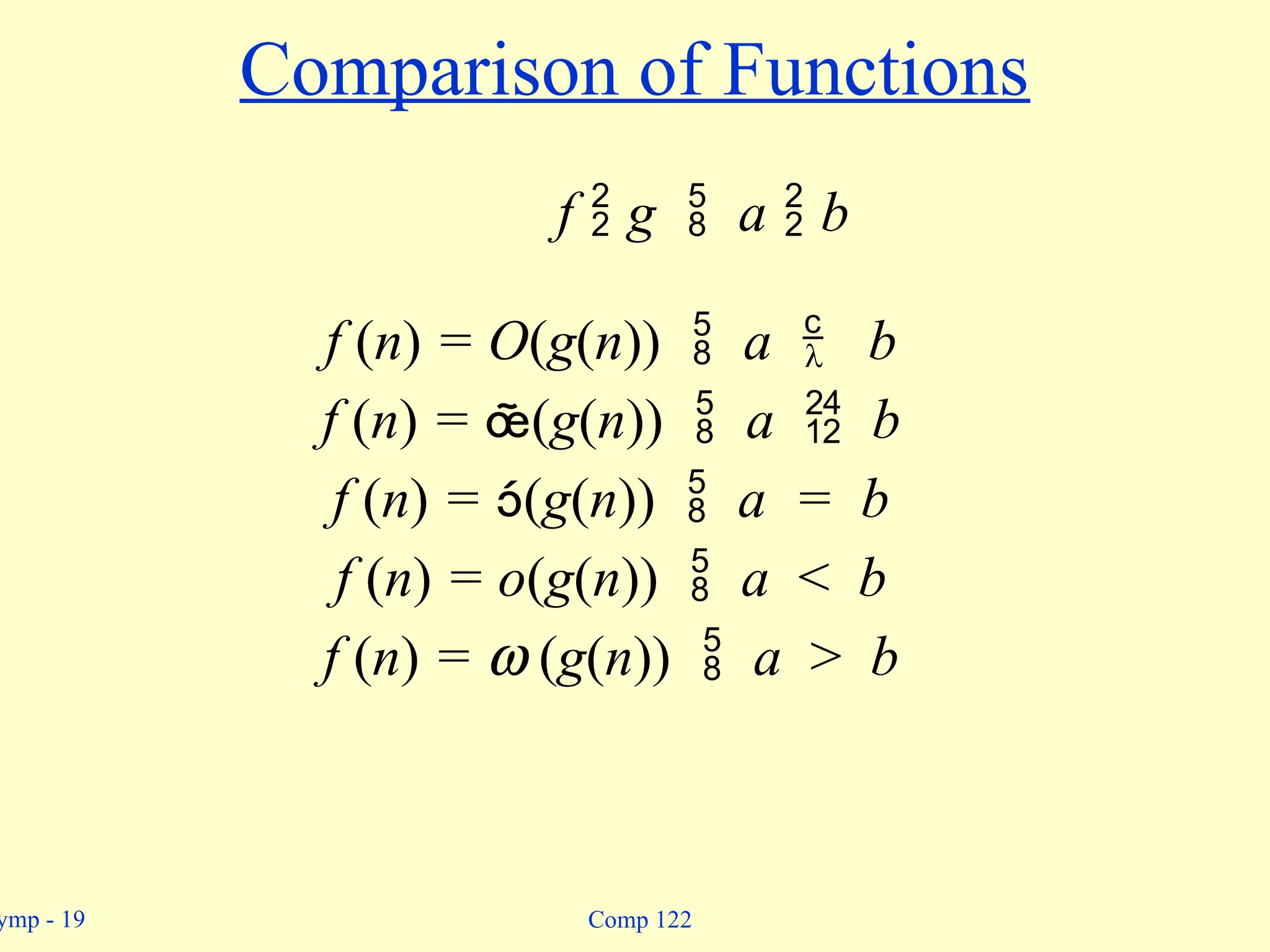
Comparison of Functions
f g a b
f (n) = O(g(n)) a b
f (n) = (g(n)) a b
f (n) = (g(n)) a = b
f (n) = o(g(n)) a < b
f (n) = w (g(n)) a > b
ymp - 24Comp 122
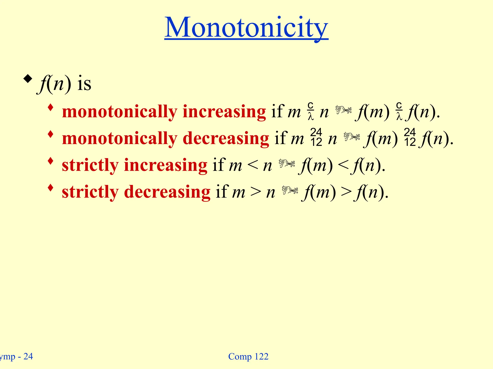
Monotonicity
f(n) is
monotonically increasing if m n f(m) f(n).
monotonically decreasing if m n f(m) f(n).
strictly increasing if m < n f(m) < f(n).
strictly decreasing if m > n f(m) > f(n).
25.
ymp - 25Comp 122
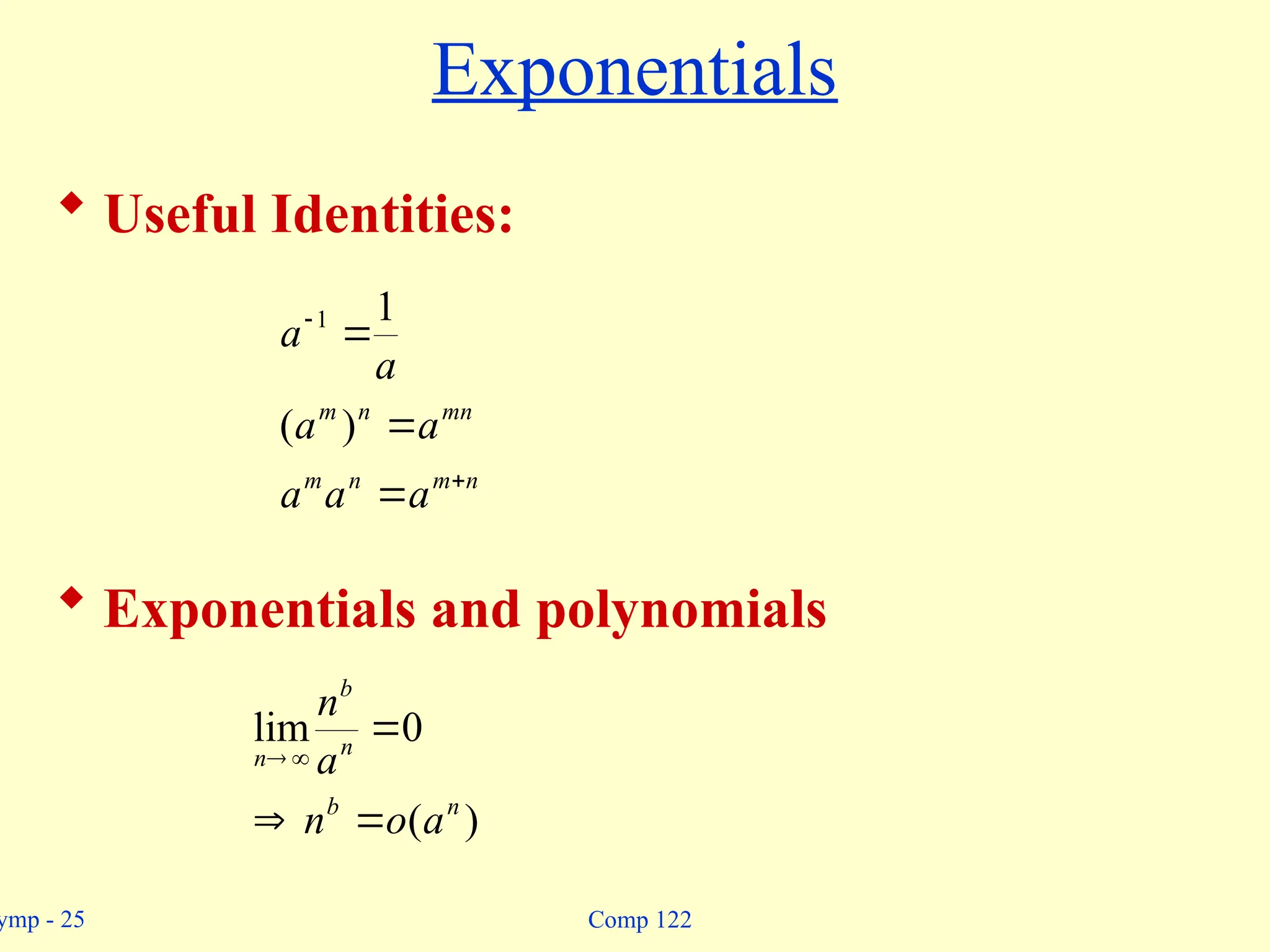
Exponentials
Useful Identities:
Exponentials and polynomials
n
m
n
m
mn
n
m
a
a
a
a
a
a
a
)
(
1
1
)
(
0
lim
n
b
n
b
n
a
o
n
a
n
26.
ymp - 26Comp 122
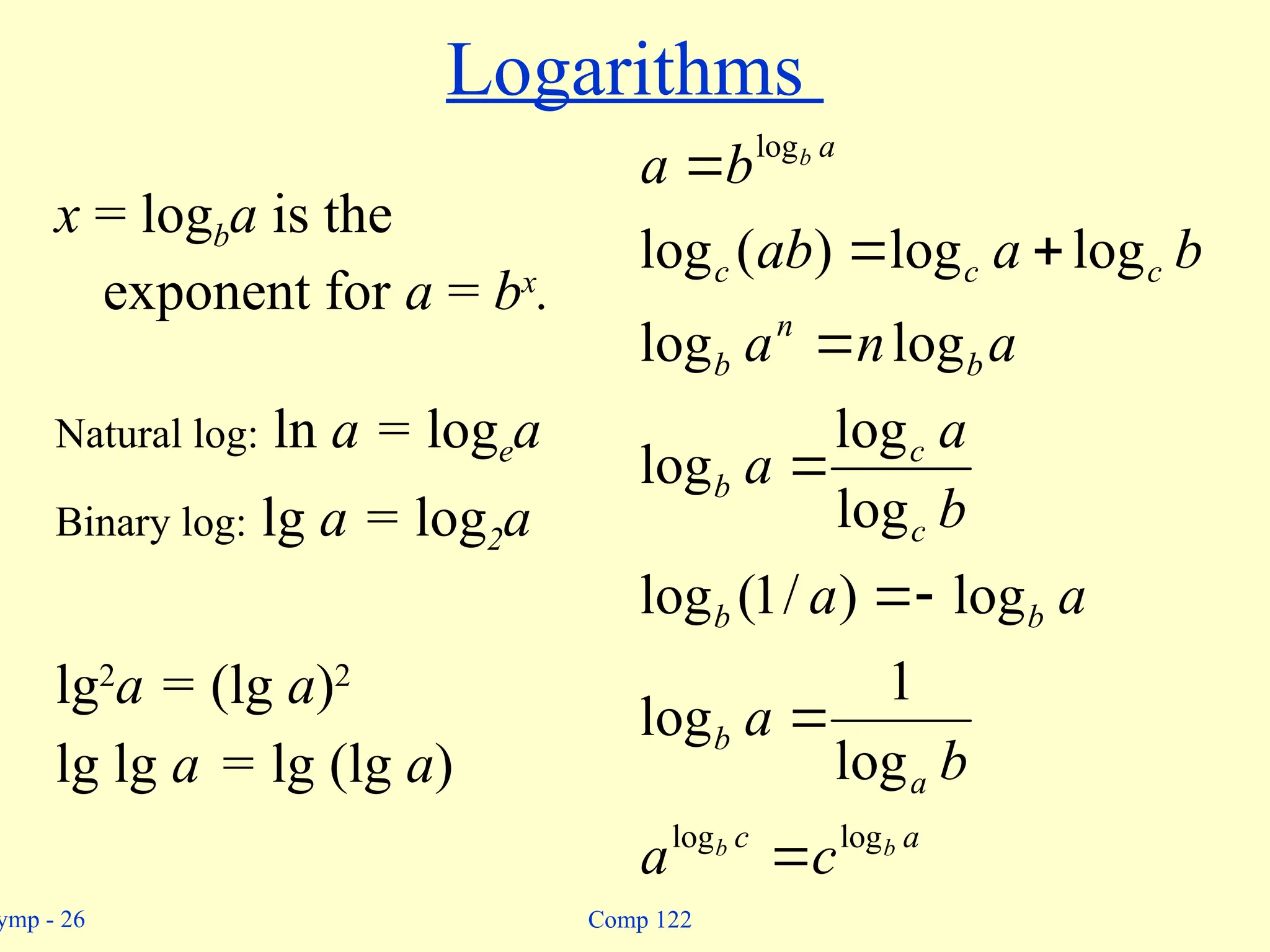
Logarithms
x = logba is the
exponent for a = bx
.
Natural log: ln a = logea
Binary log: lg a = log2a
lg2
a = (lg a)2
lg lg a = lg (lg a)
a
c
a
b
b
b
c
c
b
b
n
b
c
c
c
a
b
b
b
c
a
b
a
a
a
b
a
a
a
n
a
b
a
ab
b
a
log
log
log
log
1
log
log
)
/
1
(
log
log
log
log
log
log
log
log
)
(
log
27.
ymp - 27Comp 122
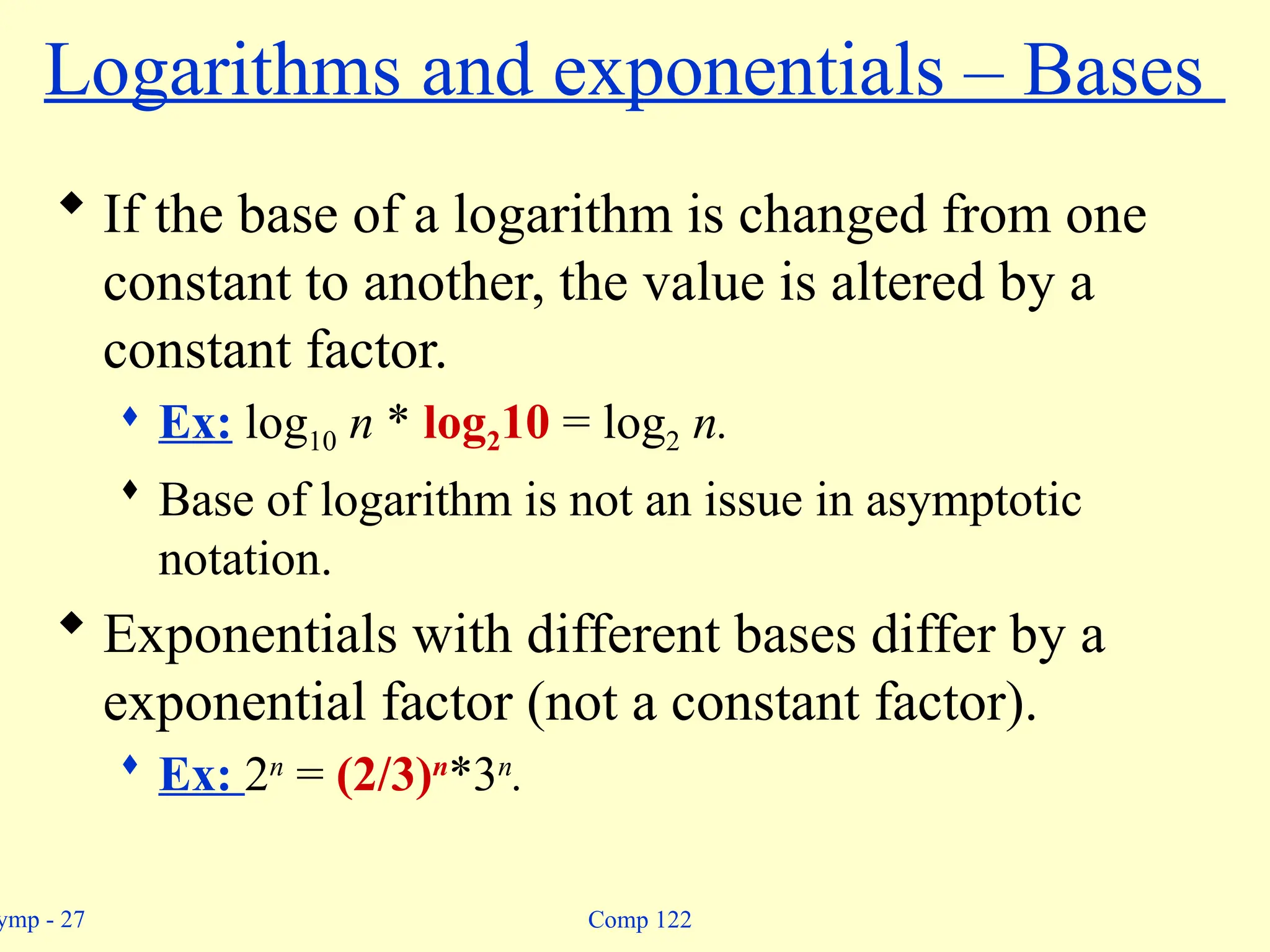
Logarithms and exponentials – Bases
If the base of a logarithm is changed from one
constant to another, the value is altered by a
constant factor.
Ex: log10 n * log210 = log2 n.
Base of logarithm is not an issue in asymptotic
notation.
Exponentials with different bases differ by a
exponential factor (not a constant factor).
Ex: 2n
= (2/3)n
*3n
.
28.
ymp - 28Comp 122
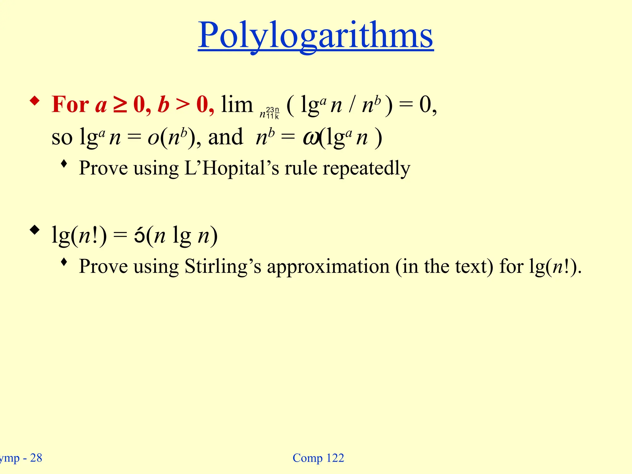
Polylogarithms
For a ³ 0, b > 0, lim n ( lga
n / nb
) = 0,
so lga
n = o(nb
), and nb
= w(lga
n )
Prove using L’Hopital’s rule repeatedly
lg(n!) = (n lg n)
Prove using Stirling’s approximation (in the text) for lg(n!).
29.
ymp - 29Comp 122
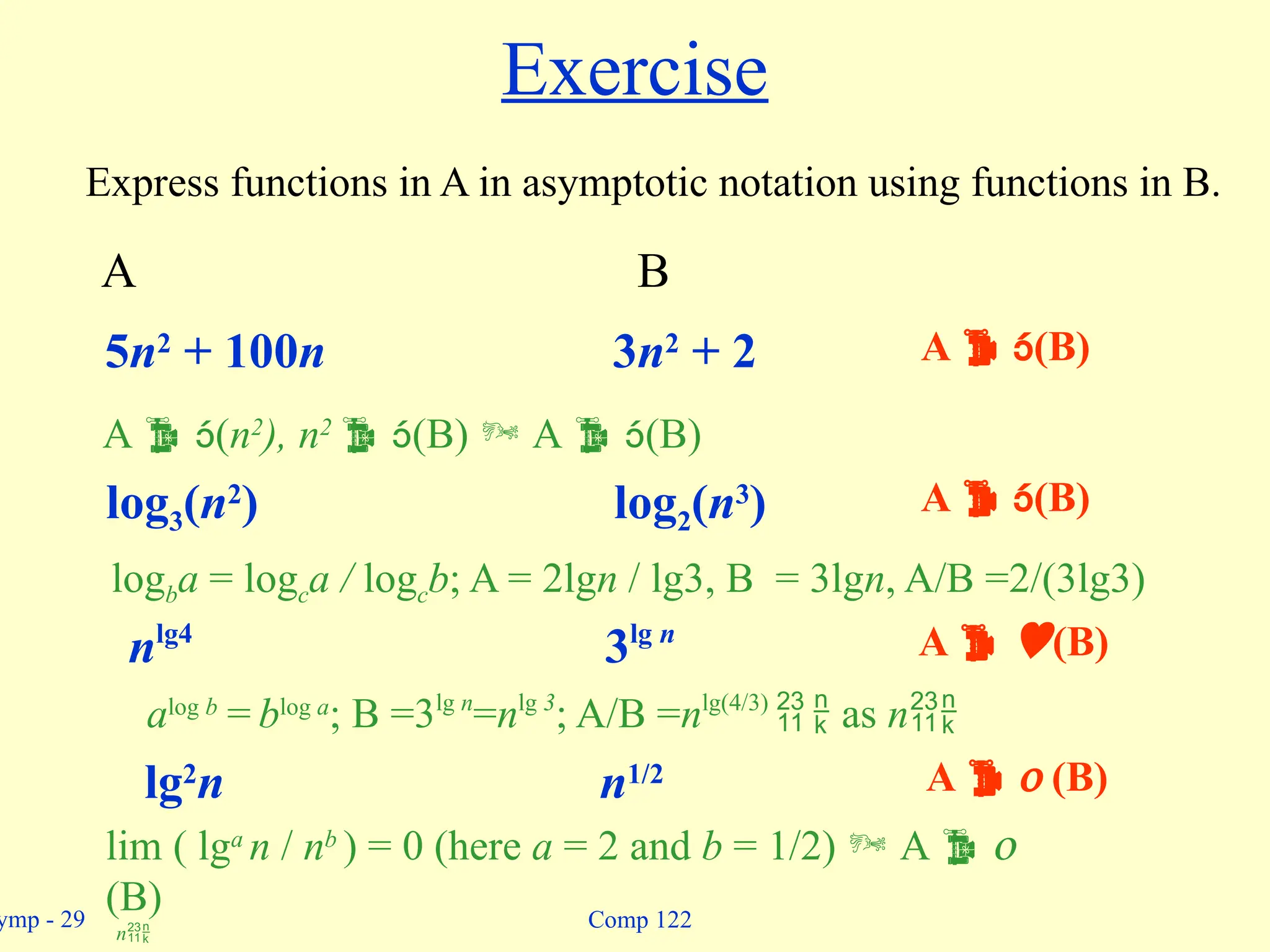
Exercise
Express functions in A in asymptotic notation using functions in B.
A B
5n2
+ 100n 3n2
+ 2
A (n2
), n2
(B) A (B)
log3(n2
) log2(n3
)
logba = logca / logcb; A = 2lgn / lg3, B = 3lgn, A/B =2/(3lg3)
nlg4
3lg n
alog b
=blog a
; B =3lg n
=nlg 3
; A/B =nlg(4/3)
as n
lg2
n n1/2
lim ( lga
n / nb
) = 0 (here a = 2 and b = 1/2) A o
(B)
n
A (B)
A (B)
A (B)
A o (B)
ymp - 31Comp 122
Review on Summations
Why do we need summation formulas?
For computing the running times of iterative
constructs (loops). (CLRS – Appendix A)
Example: Maximum Subvector
Given an array A[1…n] of numeric values (can be
positive, zero, and negative) determine the
subvector A[i…j] (1 i j n) whose sum of
elements is maximum over all subvectors.
1 -2 2 2
32.
ymp - 32Comp 122
Review on Summations
MaxSubvector(A, n)
maxsum ¬ 0;
for i ¬ 1 to n
do for j = i to n
sum ¬ 0
for k ¬ i to j
do sum += A[k]
maxsum ¬ max(sum, maxsum)
return maxsum
n n j
T(n) = 1
i=1 j=i k=i
NOTE: This is not a simplified solution. What is the final answer?
33.
ymp - 33Comp 122
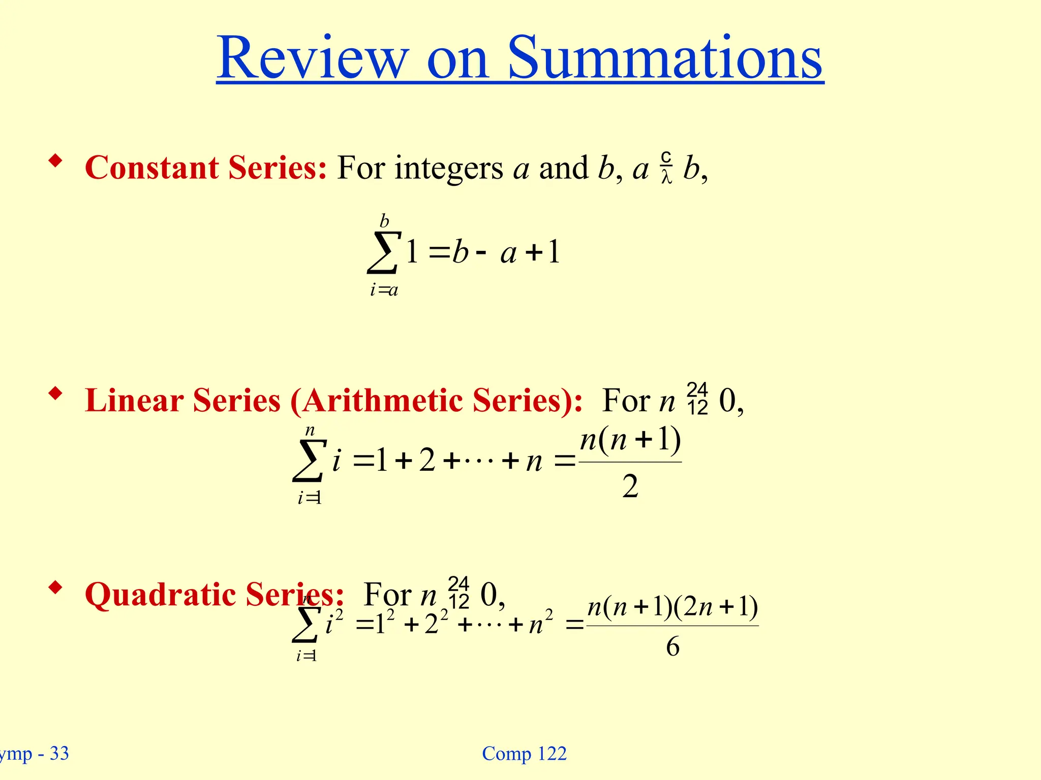
Review on Summations
Constant Series: For integers a and b, a b,
Linear Series (Arithmetic Series): For n 0,
Quadratic Series: For n 0,
b
a
i
a
b 1
1
2
)
1
(
2
1
1
n
n
n
i
n
i
n
i
n
n
n
n
i
1
2
2
2
2
6
)
1
2
)(
1
(
2
1
34.
ymp - 34Comp 122
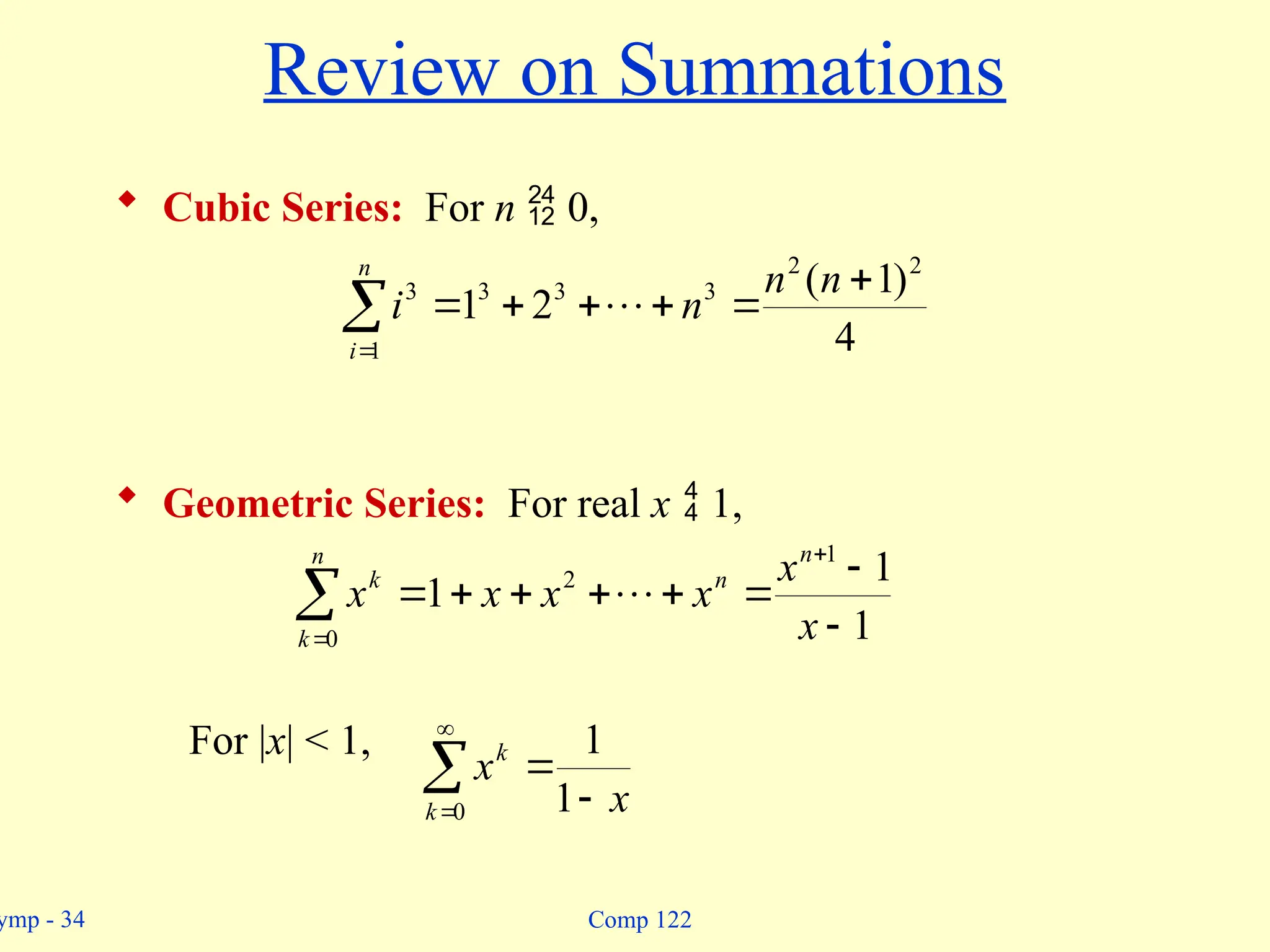
Review on Summations
Cubic Series: For n 0,
Geometric Series: For real x 1,
For |x| < 1,
n
i
n
n
n
i
1
2
2
3
3
3
3
4
)
1
(
2
1
n
k
n
n
k
x
x
x
x
x
x
0
1
2
1
1
1
0 1
1
k
k
x
x
35.
ymp - 35Comp 122
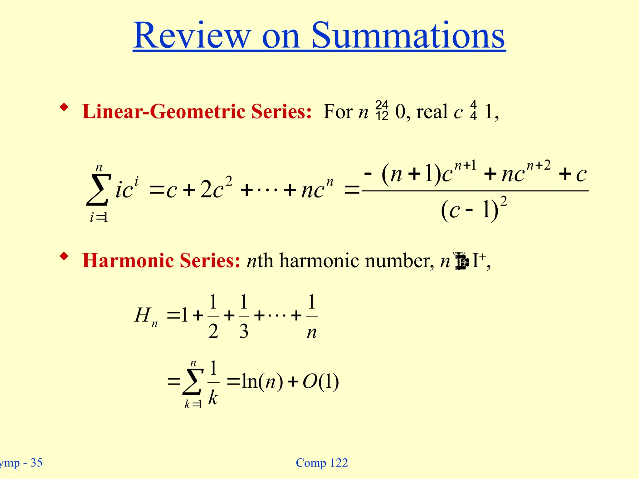
Review on Summations
Linear-Geometric Series: For n 0, real c 1,
Harmonic Series: nth harmonic number, nI+
,
n
i
n
n
n
i
c
c
nc
c
n
nc
c
c
ic
1
2
2
1
2
)
1
(
)
1
(
2
n
Hn
1
3
1
2
1
1
n
k
O
n
k
1
)
1
(
)
ln(
1
36.
ymp - 36Comp 122
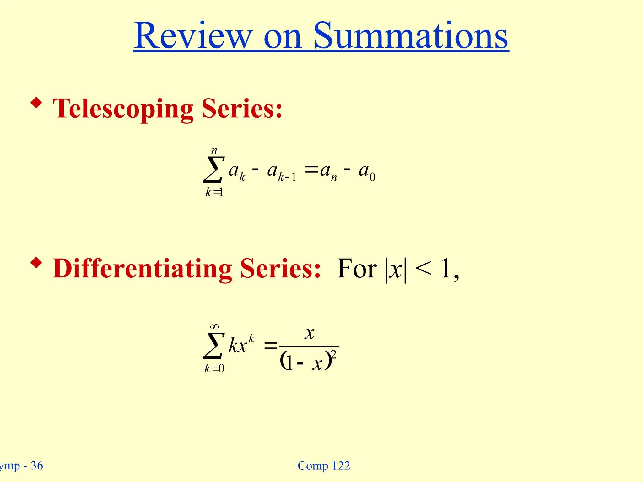
Review on Summations
Telescoping Series:
Differentiating Series: For |x| < 1,
n
k
n
k
k a
a
a
a
1
0
1
0
2
1
k
k
x
x
kx
37.
ymp - 37Comp 122
Review on Summations
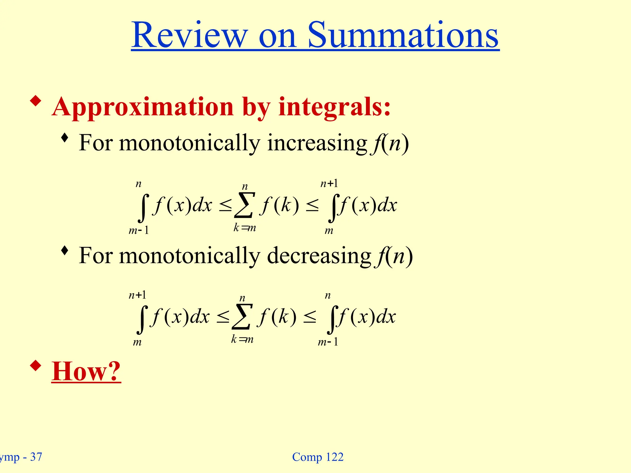
Approximation by integrals:
For monotonically increasing f(n)
For monotonically decreasing f(n)
How?
n
m
n
m
k
n
m
dx
x
f
k
f
dx
x
f
1
1
)
(
)
(
)
(
1
1
)
(
)
(
)
(
n
m
n
m
k
n
m
dx
x
f
k
f
dx
x
f
38.
ymp - 38Comp 122
Review on Summations
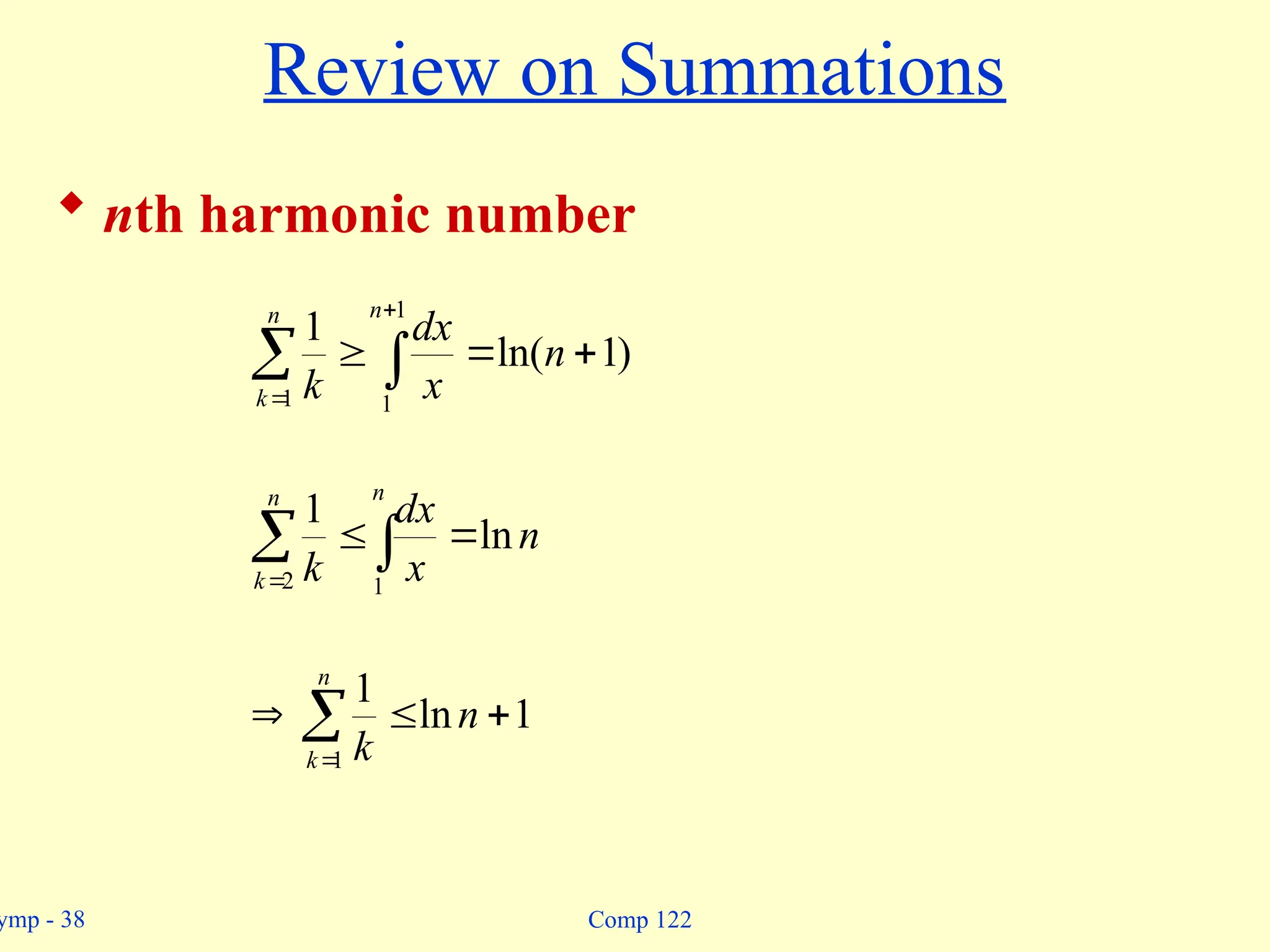
nth harmonic number
n
k
n
n
x
dx
k
1
1
1
)
1
ln(
1
n
k
n
n
x
dx
k
2 1
ln
1
n
k
n
k
1
1
ln
1
![ymp - 17 Comp 122
o-notation
f(n) becomes insignificant relative to g(n) as n
approaches infinity:
lim [f(n) / g(n)] = 0
n
g(n) is an upper bound for f(n) that is not
asymptotically tight.
Observe the difference in this definition from previous
ones. Why?
o(g(n)) = {f(n): c > 0, n0 > 0 such that
n n0, we have 0 f(n) < cg(n)}.
For a given function g(n), the set little-o:](https://image.slidesharecdn.com/asymptoticnotations-250319065846-9868ad48/75/Asymptotic-notations-for-desing-analysis-of-algorithm-pptx-17-2048.jpg)
![ymp - 18 Comp 122
w(g(n)) = {f(n): c > 0, n0 > 0 such that
n n0, we have 0 cg(n) < f(n)}.
w -notation
f(n) becomes arbitrarily large relative to g(n) as n
approaches infinity:
lim [f(n) / g(n)] = .
n
g(n) is a lower bound for f(n) that is not
asymptotically tight.
For a given function g(n), the set little-omega:](https://image.slidesharecdn.com/asymptoticnotations-250319065846-9868ad48/75/Asymptotic-notations-for-desing-analysis-of-algorithm-pptx-18-2048.jpg)
![ymp - 20 Comp 122
Limits
lim [f(n) / g(n)] = 0 Þ f(n) Î o(g(n))
n
lim [f(n) / g(n)] < Þ f(n) Î O(g(n))
n
0 < lim [f(n) / g(n)] < Þ f(n) Î Q(g(n))
n
0 < lim [f(n) / g(n)] Þ f(n) Î W(g(n))
n
lim [f(n) / g(n)] = Þ f(n) Î w(g(n))
n
lim [f(n) / g(n)] undefined Þ can’t say
n](https://image.slidesharecdn.com/asymptoticnotations-250319065846-9868ad48/75/Asymptotic-notations-for-desing-analysis-of-algorithm-pptx-20-2048.jpg)
![ymp - 31 Comp 122
Review on Summations
Why do we need summation formulas?
For computing the running times of iterative
constructs (loops). (CLRS – Appendix A)
Example: Maximum Subvector
Given an array A[1…n] of numeric values (can be
positive, zero, and negative) determine the
subvector A[i…j] (1 i j n) whose sum of
elements is maximum over all subvectors.
1 -2 2 2](https://image.slidesharecdn.com/asymptoticnotations-250319065846-9868ad48/75/Asymptotic-notations-for-desing-analysis-of-algorithm-pptx-31-2048.jpg)
![ymp - 32 Comp 122
Review on Summations
MaxSubvector(A, n)
maxsum ¬ 0;
for i ¬ 1 to n
do for j = i to n
sum ¬ 0
for k ¬ i to j
do sum += A[k]
maxsum ¬ max(sum, maxsum)
return maxsum
n n j
T(n) = 1
i=1 j=i k=i
NOTE: This is not a simplified solution. What is the final answer?](https://image.slidesharecdn.com/asymptoticnotations-250319065846-9868ad48/75/Asymptotic-notations-for-desing-analysis-of-algorithm-pptx-32-2048.jpg)