Downloaded 192 times


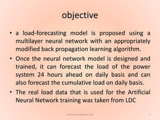


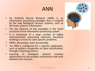


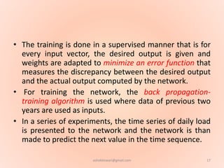

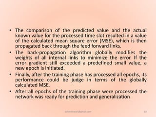

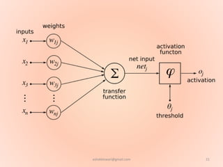
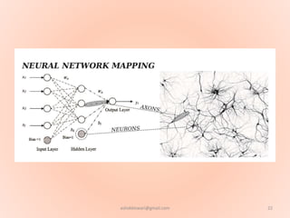

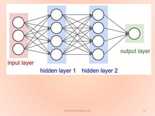

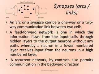


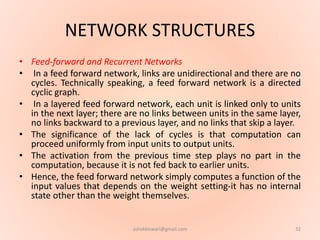
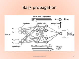
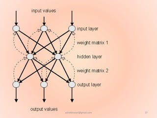


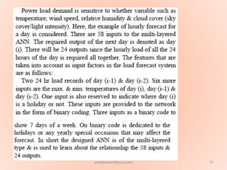


The document proposes using an artificial neural network with a modified backpropagation algorithm for load forecasting. It describes developing a model to forecast electrical load for the next 24 hours on a daily basis. The neural network is trained using historical load data from a load dispatch center. Once trained, the network can generate daily load forecasts. The document provides background on artificial neural networks, including their structure of interconnected processing units inspired by biological neurons, and how they are trained through a process of backward propagation of errors.


![Power system planning & operation [eceg 4410]](https://cdn.slidesharecdn.com/ss_thumbnails/powersystemplanningoperationeceg-4410-130607134359-phpapp01-thumbnail.jpg?width=640&height=640&fit=bounds)