This document summarizes the thermal characterization of a gas-gap heat switch developed by the University of Twente in collaboration with ESA. The heat switch uses a gas whose thermal conductivity varies with temperature and pressure to act as a thermal conductor or insulator. The author built thermal models and conducted experiments to evaluate the heat switch performance. The experimental results showed good agreement with the models. The heat switch exhibited an ON conductance of 2.60 W/K and OFF conductance of 0.30 W/K with an ON/OFF ratio of 8.67 when operating with helium gas. Improvements to the manufacturing process were also recommended to enhance performance and tolerances.

![List of Figures
Figure 1: Solar zenith angle................................................................................................... 8
Figure 2: Heat switches between components and spacecraft structure [13]..........................12
Figure 3: Heat switch between spacecraft structure and radiator [13]...................................12
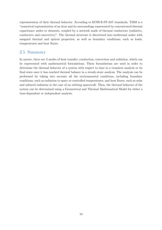
Figure 4: First prototype vertical cross-section.....................................................................13
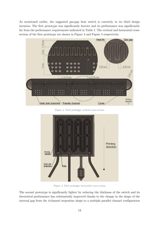
Figure 5: First prototype horizontal cross-section.................................................................13
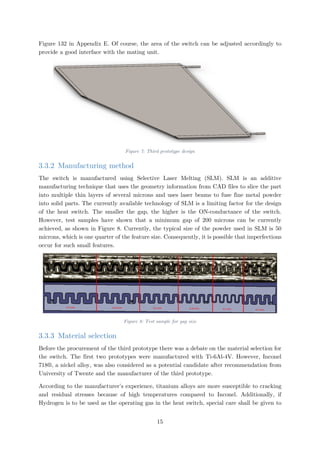
Figure 6: Second prototype horizontal cross-section .............................................................14
Figure 7: Third prototype design..........................................................................................15
Figure 8: Test sample for gap size........................................................................................15
Figure 9: Paraffin heat switch dimensions ............................................................................17
Figure 10: Total thermal conductance with temperature......................................................17
Figure 11: Starsys pedestal heat switch [13] .........................................................................17
Figure 12: IberEspacio heat switch.......................................................................................18
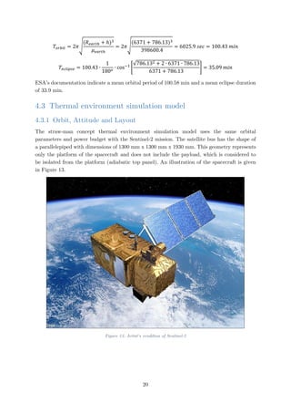
Figure 13: Artist's rendition of Sentinel-2.............................................................................20
Figure 14: Unit layout of simulation model ..........................................................................21
Figure 15: Visualization of the orbit as seen from the sun at 2800 sec..................................22
Figure 16: Units temperature profile (worst hot, no switch).................................................25
Figure 17: +Z panel temperature profile (Worst cold, no switch).........................................25
Figure 18: +Z panel temperature profile (Worst cold, with switch)......................................26
Figure 19: OFF-state thermal network.................................................................................27
Figure 20: ON-state thermal network...................................................................................29
Figure 21: Simplified ON-case thermal network ...................................................................30
Figure 22: Variation of thermal conductivity of Argon [24] ..................................................32
Figure 23: Gas thermal conductivity in the transition regime...............................................36
Figure 24: Classification of free-molecular, transition, and continuum regimes for heat
conduction across a gas confined between parallel plates [24]...............................................37
Figure 25: Convective currents in a horizontal enclosure [6].................................................38
Figure 26: A vertical rectangular enclosure with isothermal surfaces [6]...............................38
Figure 27: Infinitely large parallel plates radiation heat exchange [6] ...................................39
Figure 28: Front view of second prototype ...........................................................................42
Figure 29: Test assembly with no applied torque .................................................................42
Figure 30: Test assembly with a 1 N∙m torque....................................................................43
Figure 31: Buckling of iteration 1.........................................................................................43
Figure 32: Added stiffeners to prevent buckling ...................................................................43
Figure 33: Buckling of iteration 3.........................................................................................44
Figure 34: Iteration 4 - lattice structure for additional stiffness............................................45
Figure 35: Second prototype thickness and flatness deviation...............................................45
Figure 36: Second prototype gap size (edge).........................................................................46
Figure 37: Second prototype gap size (middle).....................................................................46
Figure 38: Second prototype support pillars .........................................................................47
Figure 39: Side views of a cracked support pillar..................................................................47
Figure 40: Remaining powder inside second prototype .........................................................48
Figure 41: CT scan setup .....................................................................................................48
vi](https://image.slidesharecdn.com/ab16c9ba-74cc-44a4-aa76-d5a97c25dce8-160912051601/85/AE5810-Thesis-6-320.jpg)
![Figure 42: Third prototype cross-section ..............................................................................49
Figure 43: Third prototype gap size .....................................................................................49
Figure 44: Third prototype pillars side views .......................................................................49
Figure 45: Third prototype channel clog ..............................................................................50
Figure 46: Third prototype channel clog cross-section..........................................................50
Figure 47: Thermoelectric cooler mounting scheme. (From FerroTec)..................................51
Figure 48: Test setup sandwich configuration.......................................................................52
Figure 49: Test setup cross-section.......................................................................................52
Figure 50: T/C placement through groove ...........................................................................53
Figure 51: Heat switch covered with MLI.............................................................................54
Figure 52: Pressure sensor calibration curve.........................................................................55
Figure 53: Pressure handling system schematic ....................................................................56
Figure 54: Bolt thermal resistance against bolt shaft diameter.............................................59
Figure 55: M4 bolt thermal resistance against plate thickness..............................................60
Figure 56: Dimensional correlation of bolted-joint conductance [13].....................................61
Figure 57: Maximum Von-Mises stresses location.................................................................68
Figure 58: Pillar cross-section stresses [5.33 bar] ..................................................................69
Figure 59: Pillar cross-section stresses [2.3 bar] ....................................................................69
Figure 60: Switch cross-section near edges (baseplate at 20o
C).............................................70
Figure 61: Switch cross-section middle (baseplate at 20o
C) ..................................................70
Figure 62: Thermal model couplings and BCs ......................................................................71
Figure 63: ON-conductance scale analysis ............................................................................72
Figure 64: OFF-conductance scale analysis ..........................................................................73
Figure 65: Heat switch area density .....................................................................................73
Figure 66: Test setup reduced thermal network ...................................................................75
Figure 67: Lumped mass test setup transient response at 20o
C (ON-case)............................76
Figure 68: FEM test setup transient response at 20o
C (ON-case).........................................76
Figure 69: Lumped mass test setup transient response at 20o
C (OFF-case)..........................77
Figure 70: FEM test setup transient response at 20o
C (OFF-case).......................................77
Figure 71: Sigraflex contact heat transfer coefficient for second prototype ...........................81
Figure 72: Sigraflex contact heat transfer coefficient for third prototype (OFF-case) ...........81
Figure 73: Sigraflex contact heat transfer coefficient for third prototype (ON-case).............82
Figure 74: Second prototype real time constant - ON-state (20o
C).......................................83
Figure 75: Second prototype ON-case transient response (20o
C)...........................................83
Figure 76: Second prototype real time constant - OFF-state (20o
C).....................................84
Figure 77: Second prototype OFF-case transient response (20o
C).........................................85
Figure 78: Third prototype real time constant - ON-state (20o
C).........................................86
Figure 79: Third prototype ON-case transient response (20o
C).............................................86
Figure 80: Third prototype real time constant - OFF-state (20o
C).......................................87
Figure 81: Third prototype OFF-case transient response (20o
C)...........................................87
Figure 82: Second prototype ON-state heat transfer coefficient (P = 40 W) ........................88
Figure 83: Exaggerated arc-shape deformation of second prototype .....................................89
Figure 84: Second prototype in-plane temperature distribution (ON-case) ...........................89
Figure 85: Second prototype ON-state overall heat transfer coefficient (Plate 1 to Plate 2).90
vii](https://image.slidesharecdn.com/ab16c9ba-74cc-44a4-aa76-d5a97c25dce8-160912051601/85/AE5810-Thesis-7-320.jpg)
![Figure 86: Third prototype ON-state heat transfer coefficient (P = 50 W) ..........................91
Figure 87: Third prototype ON-state overall heat transfer coefficient (Plate 1 to Plate 2)...91
Figure 88: Switch heat transfer coefficient (Neon)................................................................92
Figure 89: Overall heat transfer coefficient (Neon)...............................................................93
Figure 90: Effect of temperature on titanium alloys thermal conductivity............................94
Figure 91: Second prototype OFF-state heat transfer coefficient (P = 5 W)........................94
Figure 92: Second prototype OFF-state overall heat transfer coefficient (Plate 1 to Plate 2)
............................................................................................................................................95
Figure 93: Second prototype in-plane temperature distribution (OFF-case) .........................96
Figure 94: Third prototype OFF-state heat transfer coefficient (P = 15 W) ........................97
Figure 95: Third prototype OFF-state overall heat transfer coefficient (Plate 1 to Plate 2).97
Figure 96: Second prototype pressure drop...........................................................................98
Figure 97: Heat transfer coefficient against pressure (second prototype) ..............................99
Figure 98: Transition to continuum regime heat transfer coefficient (second prototype) ....100
Figure 99: Third prototype pressure drop...........................................................................100
Figure 100: Heat transfer coefficient against pressure (third prototype) .............................101
Figure 101: Third prototype ON/OFF ratio.......................................................................102
Figure 102: Third prototype ON/OFF ratio.......................................................................102
Figure 103: T/C temperature difference with calibration points (second prototype)...........106
Figure 104: Combined T/C uncertainty budget..................................................................107
Figure 105: Worst hot incident solar fluxes........................................................................109
Figure 106: Worst cold incident solar fluxes.......................................................................109
Figure 107: Units temperature profile (worst hot, no switch) .............................................111
Figure 108: Units temperature profile (worst cold, no switch)............................................111
Figure 109: +Z Panel unit temperature profile (worst cold, no switch) ..............................112
Figure 110: Units temperature profile (worst hot, no switch) .............................................112
Figure 111: Units temperature profile (worst cold, no switch)............................................113
Figure 112: +Z Panel unit temperature profile (worst cold, no switch) ..............................113
Figure 113: JUICE mission trajectory ................................................................................115
Figure 114: Fine Ti-6Al-4V powder particle size distribution .............................................116
Figure 115: Milling versus grinding process [40]..................................................................117
Figure 116: Mounting hole cross-section.............................................................................118
Figure 117: Suggested design pillar stresses........................................................................119
Figure 118: Suggested design maximum stresses (no pillars, Pgauge = 0 bar)........................120
Figure 119: Suggested design maximum stresses (no pillars, Pgauge = 1.5 bar) .................120
Figure 120: Vertical displacement at Pgauge = 1.5 bar .........................................................121
Figure 121: Side wall thickness...........................................................................................121
Figure 122: Mounting of heat switch and unit on honeycomb panel...................................122
Figure 123: Incident Albedo flux in Worst Hot ..................................................................127
Figure 124: Incident Albedo flux in Worst Cold.................................................................127
Figure 125: Incident Solar flux in Worst Hot .....................................................................128
Figure 126: Incident Solar flux in Worst Cold....................................................................128
Figure 127: Gases thermal conductivity with respect to temperature .................................131
Figure 128: Gases density with respect to temperature ......................................................131
viii](https://image.slidesharecdn.com/ab16c9ba-74cc-44a4-aa76-d5a97c25dce8-160912051601/85/AE5810-Thesis-8-320.jpg)
![Figure 129: Ratio of hemispherical emissivity to normal emittance ....................................132
Figure 130: Two infinitely long parallel strips of unequal length ........................................133
Figure 131: Second prototype fin profile.............................................................................134
Figure 132: Third prototype fin profile...............................................................................135
Figure 133: Hydrogen permeability versus temperature [42] ...............................................137
Figure 134: Bolted connections contact pressure ................................................................138
Figure 135: Test setup exaggerated displacement...............................................................139
Figure 136: Switch exaggerated displacement [2.3 bar].......................................................139
ix](https://image.slidesharecdn.com/ab16c9ba-74cc-44a4-aa76-d5a97c25dce8-160912051601/85/AE5810-Thesis-9-320.jpg)
![List of Tables
Table 1: Heat switch performance requirements...................................................................14
Table 2: IberEspacio heat switch characteristics...................................................................18
Table 3: Sentinel-2 orbital parameters [22]...........................................................................19
Table 4: Sizing cases ............................................................................................................21
Table 5: Average external fluxes on spacecraft.....................................................................22
Table 6: Model optical properties.........................................................................................23
Table 7: View Factors for internal radiation ........................................................................24
Table 8: Gebhart Factors for internal radiation ...................................................................24
Table 9: 10x10 cm2
OFF-case thermal conductances ............................................................28
Table 10: 20x20 cm2
OFF-case thermal conductances ..........................................................28
Table 11: Conductive conductances of different prototypes..................................................31
Table 12: Gas thermal conductivities at 300 K.....................................................................34
Table 13: Gases accommodation coefficients.........................................................................36
Table 14: Regime pressure limits..........................................................................................37
Table 15: Thermocouples channel and location (2nd
prototype) ............................................54
Table 16: Thermocouples channel and location (3rd
prototype..............................................54
Table 17: Fillers thermal resistance......................................................................................58
Table 18: Bolt Thermal Resistance estimate [13]..................................................................59
Table 19: Aluminium-PEEK contact heat transfer coefficient ..............................................64
Table 20: Unlubricated M4 class A2-70 socket head cap screw bolt preload parameters.......65
Table 21: Heating power leak.............................................................................................105
Table 22: Solar array thermo-optical properties .................................................................108
Table 23: Units node label..................................................................................................110
Table 24: Power subsystem components mass ....................................................................114
Table 25: Units power dissipation and temperature range..................................................126
Table 26: Acronyms, dimensions and thermal capacitance of Sentinel-2 units....................126
Table 27: Lennard-Jones constants and molecular weights of selected species [15]..............129
Table 28: Collision integrals for diffusivity, viscosity, and thermal conductivity based on the
Lennard-Jones potential [15] ..............................................................................................130
Table 29: Second prototype fin view factors.......................................................................134
Table 30: Third prototype fin view factors.........................................................................135
Table 31: Ti-6Al-4V chemical composition.........................................................................136
Table 32: Inconel 718® chemical composition.....................................................................136
Table 33: Material thermal properties................................................................................136
Table 34: Material structural properties.............................................................................136
Table 35: Classical rule-of-thumb safety factors [30]...........................................................138
x](https://image.slidesharecdn.com/ab16c9ba-74cc-44a4-aa76-d5a97c25dce8-160912051601/85/AE5810-Thesis-10-320.jpg)


![1 Introduction
1.1 General introduction
Space is a very harsh and unforgiving environment. Within a few minutes, the temperature of
a spacecraft can vary from -130o
C when in eclipse to +100o
C when in full illumination [1].
Such variations can cause permanent damage to spacecraft equipment. The Satellite Thermal
Control (STC) subsystem is an integral part of a spacecraft architecture, dedicated to
managing and controlling such variations. More specifically, STC maintains spacecraft
components within their respective temperature limits in the environments encountered during
launch and on-orbit, it maintains stable temperatures over time and ensures temperature
uniformity for sensitive components by controlling the temperature gradients.
Heat switches are an innovative, variable thermal conductance technology that can ideally
provide an adiabatic interface in order to couple or de-couple thermal surfaces according to
needs [2]. It is a technology that has not been extensively used in the thermal architecture of
past spacecraft due to their bulky structure and complexity.
In collaboration with ESA, University of Twente has developed a gas-gap heat switch that is
produced using 3D-printing technology. The suggested heat switch is easier and more
economical to produce and contains no moving parts, when compared to its state-of-the-art
counterparts. The switch allows for the thermal coupling and the de-coupling of a unit from a
heat sink (radiator) depending on the unit’s temperature. When the unit exceeds its maximum
threshold temperature, the switch is turned on so as to allow for heat to flow from the hot
unit to the radiator by conduction through an acting gas (ideally Hydrogen or Helium).
Subsequently, the heat is released into space via the radiator. When, the unit is below its
minimum threshold, the switch is turned off, being depressurized to high vacuum conditions
(<10-3
mbar), to thermally isolate the unit from the radiator.
The suggested gas-gap heat switch design is currently in its third design iteration. The first
and second prototype have already been tested at an operating temperature of 295 K and the
performance has been documented in reference [3]. However, it should be noted that the
performance of the switch is dependent on temperature due to radiative effects and the
variation of the gases thermal conductivity with temperature. This thesis is dedicated to
evaluating the thermal performance of the second and third prototype of the developed gas-
gap heat switch with respect to the operating temperature and pressure. The research objective
is to evaluate the impact of the developed gas-gap heat switch in Earth-Observation missions
and thermally characterize it. This is achieved by using a straw-man concept system analysis
and by carrying out performance quantitative tests and correlating the results to theoretical
data from Finite Element Models and reduced Thermal Mathematical Models for validation.
This thesis work can be used as a reference for the design improvement of the developed gas-
gap heat switch and as a benchmark to conduct further objective testing for the evaluation of
the performance of the future iterations. It provides a detailed report of the critical parameters
involved in this technology and of the steps taken, starting from the theoretical molecular
1](https://image.slidesharecdn.com/ab16c9ba-74cc-44a4-aa76-d5a97c25dce8-160912051601/85/AE5810-Thesis-14-320.jpg)
![5. What are the differences, advantages/disadvantages between the suggested gas-gap
heat switch and other similar thermal control means?
1.3 Hypothesis and methodology
The hypothesis to be tested is: “The developed gas-gap heat switch is beneficial to a spacecraft
in Earth-Observation missions for its thermal control.”
The initial step for the validation or not of this hypothesis is to determine the evaluation
criteria of the gas-gap heat switch. These criteria have been established by performing a
literature study on other similar heat switches.
The use of a Systems Engineering approach is necessary in order to determine the changes in
the thermal subsystem architecture and its interrelation with other subsystems. A straw-man
concept analysis based on typical Earth-Observation mission parameters will be implemented
in order to obtain some initial quantitative results, so as to determine the affected subsystems
and the extent of these effects, either positive or negative. The main expected effects concern
the mass and the power consumption.
For the thermal characterization of the switch, a FEM of the switch is required so as to have
an initial estimate of the anticipated results. This model will make use of the basic
thermodynamic and heat transfer concepts. Additionally, a FEM of the experimental setup,
including the vacuum chamber, test equipment and the switch is required in order to have
initial estimations for the results. This is a standard procedure followed by ESA before testing.
Extensive “elegant breadboard” testing is required to evaluate the performance of the heat
switch. Elegant Breadboard is an equipment between Breadboard Model and Engineering
Model. It is built using commercial grade components and a configuration close to that of the
Flight Model. The purpose of the testing is to perform breadboard validation in laboratory
environment to achieve concept-enabling levels of performance. The validations is relatively
“low-fidelity” compared to the eventual system [4].
Thermal balance tests are conducted under steady state or dynamic conditions to correlate
and adjust the FEM and TMM and verify the thermal design [5]. Due to the nature of the
tested component, simple manual correlation techniques will be used instead of more
complicated methods, such as Monte Carlo simulations, Genetic Algorithms or Adaptive
Particle Swarm Optimization.
1.4 Structure of the report
This thesis report begins by providing essential information about the fundamentals of heat
transfer and the thermal environment encountered by a spacecraft. It also outlines the methods
used to build a thermal model of a spacecraft within its environment by applying these heat
transfer fundamentals. In Chapter 3, an overview of the heat switches technology is provided,
along with the measures of effectiveness of the technology and its potential applications. In
the same chapter, the design concept of the developed gas-gap heat switch is given, as well as
3](https://image.slidesharecdn.com/ab16c9ba-74cc-44a4-aa76-d5a97c25dce8-160912051601/85/AE5810-Thesis-16-320.jpg)
![2 Fundamentals of Heat Transfer
There are 3 modes of heat transfer; conduction, convection and radiation. This chapter briefly
explains the fundamentals behind the three heat transfer modes, it defines what is steady-state
and transient analysis and provides the basic understanding of a spacecraft thermal
environment. In its last section it briefly introduces the methods used to generate mathematical
models for thermal analysis.
2.1 Modes of heat transfer
2.1.1 Conduction
Conduction is the transfer of heat energy by collision of particles with different energy levels.
Conduction occurs through a body and at the point of contact of different bodies. It is the
dominant mode of heat transfer inside the spacecraft.
Conduction can be represented using Fourier’s Law as follows [6]:
𝑄𝑄̇ = −
𝑘𝑘 ∙ 𝐴𝐴
𝑙𝑙
∙ 𝛥𝛥𝛥𝛥 [𝑊𝑊] (2.1-1)
Where 𝑘𝑘 represents the thermal conductivity, 𝐴𝐴 is the cross-sectional area, 𝑙𝑙 is the length of
the conductive path and 𝛥𝛥𝛥𝛥 is the temperature difference between two nodes. The linear
conductive conductance is represented by 𝐺𝐺𝐺𝐺 =
𝑘𝑘∙𝐴𝐴
𝑙𝑙
�
𝑊𝑊
℃
=
𝑊𝑊
𝐾𝐾
�, while the conductive thermal
resistance is its inverse 𝑅𝑅𝑐𝑐𝑐𝑐𝑐𝑐𝑐𝑐𝑐𝑐𝑐𝑐𝑐𝑐𝑐𝑐𝑣𝑣𝑒𝑒 =
𝑙𝑙
𝑘𝑘∙𝐴𝐴
�
℃
𝑊𝑊
�
For the interface between two parts, it is really important to take into account the contact
thermal conductance or its inverse, the contact thermal resistance. The contact conductance
can only be determined accurately through experimentation and depends on parameters such
as the surface and thermal properties of the materials in contact, the applied contact pressure
etc. For more details, you can refer to section 7.4.
2.1.2 Convection
Convection refers to heat transfer occurring from a solid surface to the adjacent fluid or vice
versa. Even though convection is typically absent in space due to vacuum, it is sometimes
present inside the spacecraft.
Convective heat transfer is represented with the following equation [6]:
𝑄𝑄̇ = ℎ ∙ 𝐴𝐴 ∙ 𝛥𝛥𝛥𝛥 [𝑊𝑊] (2.1-2)
Where ℎ represents the convective heat transfer coefficient in [𝑊𝑊 𝑚𝑚2
∙ 𝐾𝐾⁄ ]. The convective heat
transfer coefficient can be determined experimentally or approximated using correlations that
take into account the system geometry and the effects of buoyancy, kinematic viscosity,
thermal diffusivity and inertial forces. Such correlations can be obtained from literature, such
as reference [6], depending on whether forced or free convection occurs. In the case of the
latter, different correlations exist for internal and external flows. Similarly to conduction,
5](https://image.slidesharecdn.com/ab16c9ba-74cc-44a4-aa76-d5a97c25dce8-160912051601/85/AE5810-Thesis-18-320.jpg)
![because convection exhibits a linear behavior, the convective coupling can be represented using
𝐺𝐺𝐺𝐺 = ℎ ∙ 𝐴𝐴.
2.1.3 Radiation
Radiation is the energy emitted by a body in the form of electromagnetic waves and thus, it
does not require the presence of an intervening medium [6]. Radiation is the only way to
dissipate the energy outside the spacecraft, since the radiative environment serves as a heat
sink that absorbs the heat.
The radiative heat transfer between two surfaces 𝑖𝑖 and 𝑗𝑗 is represented using the Stefan-
Boltzmann Law [7]:
𝑄𝑄̇ = 𝜀𝜀𝑖𝑖 ∙ 𝐴𝐴𝑖𝑖 ∙ 𝜎𝜎 ∙ 𝐹𝐹𝑖𝑖𝑖𝑖 ∙ �𝛵𝛵𝑖𝑖
4
− 𝛵𝛵𝑗𝑗
4
� [𝑊𝑊] (2.1-3)
Where 𝜀𝜀𝑖𝑖 is the emissivity of surface 𝑖𝑖, 𝐴𝐴𝑖𝑖 is the area of surface 𝑖𝑖, 𝜎𝜎 = 5.67 ∙ 10−8 [𝑊𝑊 𝑚𝑚2
∙ 𝐾𝐾4⁄ ]
is the Stefan-Boltzmann constant, 𝐹𝐹𝑖𝑖𝑖𝑖 is the view factor of surface 𝑗𝑗 as seen from surface 𝑖𝑖. The
view factor is dependent on the area of the two surfaces and their geometry with respect to
each other. It can be calculated using mathematical formulas from literature, such as references
[8], [7] or using a GMM developed with computer software, such as NX Unigraphics or
ESATAN-TMS. In order to obtain more accurate results, the reflections off the surfaces shall
be taken into account. To correct for reflections, the Gebhart factor is introduced [9], [10]:
𝐵𝐵𝑖𝑖𝑖𝑖 = 𝐹𝐹𝑖𝑖𝑖𝑖 ∙ 𝜀𝜀𝑗𝑗 + �(1 − 𝜀𝜀𝑘𝑘)
𝑛𝑛
𝑘𝑘=1
∙ 𝐹𝐹𝑖𝑖𝑖𝑖 ∙ 𝐵𝐵𝑖𝑖𝑖𝑖 (2.1-4)
For complicated geometries, where more than 3 nodes are taken into account, software such
as Therm XL, can calculate the Gebhart factors if provided with the view factors and the
optical properties of the surfaces. The eventual radiative thermal conductance is [9]:
𝐺𝐺𝐺𝐺𝑖𝑖𝑖𝑖 = 𝜀𝜀𝑖𝑖 ∙ 𝐴𝐴𝑖𝑖 ∙ 𝐵𝐵𝑖𝑖𝑖𝑖 = 𝜀𝜀𝑗𝑗 ∙ 𝐴𝐴𝑗𝑗 ∙ 𝐵𝐵𝑗𝑗𝑗𝑗 [𝑚𝑚2] (2.1-5)
Equation (2.1-4) is iterative and can be simplified to a matrix equation [11]:
[𝐵𝐵] = {[𝐼𝐼] − [𝐹𝐹] + [𝐹𝐹][𝐸𝐸]} −1[𝐹𝐹][𝐸𝐸] (2.1-6)
where [𝐵𝐵] is the Gebhart factor matrix, [𝐸𝐸] is the surface emissivity matrix, [𝐹𝐹] is the view
factor matrix and [𝐼𝐼] is the identity matrix. Eventually, the radiative heat transfer equation
can be written as:
𝑄𝑄𝚤𝚤𝚤𝚤
̇ = 𝐺𝐺𝐺𝐺𝑖𝑖𝑖𝑖 ∙ �𝜎𝜎𝛵𝛵𝑖𝑖
4
− 𝜎𝜎𝛵𝛵𝑗𝑗
4
� [𝑊𝑊] (2.1-7)
6](https://image.slidesharecdn.com/ab16c9ba-74cc-44a4-aa76-d5a97c25dce8-160912051601/85/AE5810-Thesis-19-320.jpg)
![2.2 Steady-state and Transient Analysis
2.2.1 Steady-state Analysis
Steady-state analysis is independent of time and expresses the temperature when heat balance
has been achieved throughout the system. The general steady-state differential equation is
given by [12]:
0 = Qi
𝑒𝑒𝑒𝑒𝑒𝑒𝑒𝑒𝑒𝑒𝑒𝑒𝑒𝑒𝑒𝑒
+ 𝑄𝑄𝑖𝑖
𝑖𝑖𝑖𝑖𝑖𝑖𝑖𝑖𝑖𝑖𝑖𝑖𝑖𝑖𝑖𝑖
− � 𝐺𝐺𝐿𝐿𝑖𝑖𝑖𝑖�𝑇𝑇𝑖𝑖 − 𝑇𝑇𝑗𝑗�
𝑗𝑗
− � 𝐺𝐺𝑅𝑅𝑖𝑖𝑖𝑖(𝜎𝜎𝑇𝑇𝑖𝑖
4
− 𝜎𝜎𝜎𝜎𝑗𝑗
4
)
𝑗𝑗
(2.2-1)
where Qi
𝑒𝑒𝑒𝑒𝑒𝑒𝑒𝑒𝑒𝑒𝑒𝑒𝑒𝑒𝑒𝑒
and 𝑄𝑄𝑖𝑖
𝑖𝑖𝑖𝑖𝑖𝑖𝑖𝑖𝑖𝑖𝑖𝑖𝑖𝑖𝑖𝑖
represent the external heat power and internal power dissipation.
2.2.2 Transient Analysis
Transient analysis is dependent on time and expresses the temperatures at every time-step 𝛥𝛥𝛥𝛥
used in the calculations. The general differential equation for the transient analysis is:
𝐶𝐶𝑖𝑖
𝜕𝜕𝑇𝑇𝑖𝑖
𝜕𝜕𝜕𝜕
= Qi
𝑒𝑒𝑒𝑒𝑒𝑒𝑒𝑒𝑒𝑒𝑒𝑒𝑒𝑒𝑒𝑒
+ 𝑄𝑄𝑖𝑖
𝑖𝑖𝑖𝑖𝑖𝑖𝑖𝑖𝑖𝑖𝑖𝑖𝑖𝑖𝑖𝑖
− � 𝐺𝐺𝐿𝐿𝑖𝑖𝑖𝑖�𝑇𝑇𝑖𝑖 − 𝑇𝑇𝑗𝑗�
𝑗𝑗
− � 𝐺𝐺𝑅𝑅𝑖𝑖𝑖𝑖(𝜎𝜎𝑇𝑇𝑖𝑖
4
− 𝜎𝜎𝜎𝜎𝑗𝑗
4
)
𝑗𝑗
(2.2-2)
where 𝐶𝐶𝑖𝑖 = 𝜌𝜌𝑖𝑖 ∙ 𝐶𝐶𝑝𝑝𝑖𝑖 ∙ 𝑉𝑉𝑖𝑖 [𝐽𝐽 𝐾𝐾⁄ ] is the thermal capacitance of body 𝑖𝑖, 𝜌𝜌𝑖𝑖 is its density [𝑘𝑘𝑘𝑘/𝑚𝑚3
],
𝐶𝐶𝑝𝑝𝑖𝑖 is the specific heat [𝐽𝐽 𝑘𝑘𝑔𝑔 ∙ 𝐾𝐾⁄ ] and 𝑉𝑉𝑖𝑖 [𝑚𝑚3] is the body’s volume. The heat capacity expresses
the amount of heat required to change the temperature of a body by 1o
C.
Under the same conditions, if a transient analysis is given adequate time, it always results in
a plateau temperature that is equal to the steady-state solution. Mathematically, this equation
exhibits an asymptotic behavior. Transient analysis is necessary in order to obtain the thermal
behavior of a spacecraft during illumination and eclipse. Transient analysis is also used for
thermal fatigue and thermal cycling calculations.
2.3 Spacecraft thermal environment
2.3.1 Solar Radiation
Solar radiation is the result of the Sun acting as an almost perfect black-body, emitting
radiation according to Planck’s Black-body Radiation Law. A black-body is an ideal body that
allows all the incident radiation to pass into it (no reflected energy) and internally absorbs all
the incident radiation (no transmitted energy) for all wavelengths and angles of incidence [7].
Same conditions apply for the emitted energy from a black-body. The received solar radiation
on Earth and on orbits around Earth varies because of the elliptical orbit of Earth around the
Sun. The minimum solar flux is 1322 W/m2
at the summer solstice and the maximum solar
flux is at 1414 W/m2
at the winter solstice [13]. Using Wien’s displacement Law for an average
sun temperature of 5770 K, we observe that most of the solar radiation is emitted at 0.5 μm
and in the range of visible spectrum [14].
𝜆𝜆 𝑚𝑚𝑚𝑚𝑚𝑚[𝜇𝜇𝜇𝜇] =
2900
𝑇𝑇
=
2900
5770
= 0.5 𝜇𝜇𝜇𝜇 (2.3-1)
7](https://image.slidesharecdn.com/ab16c9ba-74cc-44a4-aa76-d5a97c25dce8-160912051601/85/AE5810-Thesis-20-320.jpg)
![2.3.2 Albedo
Some of the incoming sunlight is reflected off a planet. Albedo (or Bond Albedo) is the ratio
of the reflected/scattered radiation and the total incoming radiation integrated over frequency.
On Earth, albedo varies over areas with land or oceans and generally increases with increasing
cloud coverage and increasing latitude. Consequently, the orbit inclination affects the Albedo.
Thus, it is always a great challenge for a thermal engineer to decide the albedo parameters of
the analysis. Albedo can vary from 0.1 to 0.5 over different orbits and a value of 0.2 and 0.4
can be typically used for the worst cold and worst hot scenario respectively. Albedo, has the
same spectral distribution as sunlight, but is not completely diffusive. The absorbed albedo
flux on a surface is calculated as [13]:
𝛷𝛷𝑎𝑎𝑎𝑎𝑎𝑎𝑎𝑎𝑑𝑑𝑑𝑑 = 𝛼𝛼 ∙ 𝐴𝐴𝑏𝑏 ∙ 𝐹𝐹𝑝𝑝𝑝𝑝𝑝𝑝𝑝𝑝𝑝𝑝𝑝𝑝 ∙ 𝛷𝛷𝑠𝑠𝑠𝑠𝑠𝑠𝑠𝑠𝑠𝑠 ∙ cos 𝜃𝜃 (2.3-2)
𝛼𝛼 is the absorptivity of the surface, 𝐴𝐴𝑏𝑏 is the bond albedo, 𝐹𝐹𝑝𝑝𝑝𝑝𝑝𝑝𝑝𝑝𝑝𝑝𝑝𝑝 is the view factor of the
surface to the planet and 𝛷𝛷𝑠𝑠𝑠𝑠𝑠𝑠𝑠𝑠𝑠𝑠 is the solar flux. cos 𝜃𝜃 is the solar zenith angle that the sun
rays form with sub-satellite point and the satellite, as shown in Figure 1.
Figure 1: Solar zenith angle1
The solar zenith angle is given by:
cos 𝜃𝜃 = sin 𝛷𝛷 sin 𝛿𝛿 + cos 𝛷𝛷 cos 𝛿𝛿 cos ℎ (2.3-3)
𝛷𝛷, 𝛿𝛿, ℎ are the local latitude, the current declination of the sun and the hour angle in local
solar time respectively.
2.3.3 Planetary Radiation
A planet absorbs the solar radiation that is not scattered or reflected due to albedo. This
energy is re-emitted by the planet according to the Black-body Radiation Law. Earth has an
average equilibrium temperature of -18o
C (255 K), which can in general vary from 240 K to
260 K, depending on the solar constant and the Albedo assumptions. Using Wien’s
1
Picture obtained from Landsat 7 Handbook
8](https://image.slidesharecdn.com/ab16c9ba-74cc-44a4-aa76-d5a97c25dce8-160912051601/85/AE5810-Thesis-21-320.jpg)
![Displacement Law, we observe that Earth emits most of its radiation at 11.4 μm, i.e. in the
infra-red spectrum. According to Kirchhoff’s Law in its diffuse form, a good emitter is a good
absorber at a particular wavelength or at a specific range of wavelengths, i.e. 𝛼𝛼𝜆𝜆 = 𝜀𝜀𝜆𝜆 [15].
Because of the temperature variations on the Earth’s surface, the emitted infra-red radiation
fluxes fluctuate. IR fluxes typically range from 150 to 350 W/m2
. The absorbed IR flux on a
surface is calculated [13]:
𝛷𝛷𝐼𝐼 𝐼𝐼 = 𝜀𝜀𝑠𝑠𝑠𝑠𝑠𝑠𝑠𝑠𝑠𝑠𝑐𝑐𝑐𝑐 ∙ 𝜀𝜀𝑝𝑝𝑝𝑝𝑝𝑝𝑝𝑝𝑝𝑝𝑝𝑝 ∙ 𝐹𝐹𝑝𝑝𝑝𝑝𝑝𝑝𝑝𝑝𝑝𝑝𝑝𝑝 ∙ 𝜎𝜎 ∙ 𝑇𝑇𝑝𝑝𝑝𝑝𝑝𝑝𝑝𝑝𝑝𝑝𝑝𝑝
4
(2.3-4)
𝜀𝜀𝑠𝑠𝑠𝑠𝑠𝑠𝑠𝑠𝑠𝑠𝑠𝑠𝑠𝑠 𝑖𝑖s the emissivity of the surface, 𝜀𝜀𝑝𝑝𝑝𝑝𝑝𝑝𝑝𝑝𝑝𝑝𝑝𝑝 is the emissivity of the planet and is equal to
1 since Earth is treated as a black body, 𝐹𝐹𝑝𝑝𝑝𝑝𝑝𝑝𝑝𝑝𝑝𝑝𝑝𝑝 is the view factor of the surface to the planet,
𝜎𝜎 = 5.67 ∙ 10−8 [𝑊𝑊 𝑚𝑚2
∙ 𝐾𝐾4⁄ ] is the Stefan-Boltzmann constant and 𝑇𝑇𝑝𝑝𝑝𝑝𝑝𝑝𝑝𝑝𝑝𝑝𝑝𝑝 is the temperature
of the planet.
2.3.4 Low-Earth Orbit Environment
LEO are typical of Earth-Observation missions, as most instruments require close proximity
to the target for better resolution and measurements. Altitudes vary from 200 km to 2000 km,
but most of the LEO satellites are in the range of 400 km to 800 km. Due to their proximity
to Earth, such missions are strongly affected by Earth’s albedo and IR. LEO are circular orbits
and their orbital period can be found as [14]:
𝑇𝑇𝑜𝑜𝑜𝑜𝑜𝑜𝑜𝑜𝑜𝑜 = 2𝜋𝜋�
(𝑅𝑅𝑒𝑒𝑒𝑒𝑒𝑒𝑒𝑒ℎ + ℎ)3
𝜇𝜇𝑒𝑒𝑒𝑒𝑒𝑒𝑒𝑒ℎ
[𝑠𝑠𝑠𝑠𝑠𝑠] (2.3-5)
Where 𝑅𝑅𝑒𝑒𝑒𝑒𝑒𝑒𝑒𝑒ℎ = 6371 𝑘𝑘𝑘𝑘 is the radius of the Earth, ℎ [𝑘𝑘𝑘𝑘] is the altitude and 𝜇𝜇𝑒𝑒𝑒𝑒𝑒𝑒𝑒𝑒ℎ =
398600.4 𝑘𝑘𝑚𝑚3
/𝑠𝑠2
is the Earth’s gravitational parameter.
The eclipse time for a circular orbit can be calculated as [13]:
𝑇𝑇𝑒𝑒𝑒𝑒𝑒𝑒𝑒𝑒𝑒𝑒𝑒𝑒𝑒𝑒 = 𝑇𝑇𝑜𝑜𝑜𝑜𝑜𝑜𝑜𝑜𝑜𝑜 ∙
1
180𝑜𝑜
∙ cos−1
�
�ℎ2 + 2 ∙ 𝑅𝑅𝑒𝑒𝑒𝑒𝑒𝑒𝑒𝑒ℎ ∙ ℎ
(𝑅𝑅𝑒𝑒𝑒𝑒𝑒𝑒𝑒𝑒ℎ + ℎ) cos 𝛽𝛽
� (2.3-6)
𝛽𝛽 is the orbit beta angle defined as [13]:
𝛽𝛽 = sin−1(cos 𝛿𝛿𝑠𝑠 sin 𝑅𝑅𝑅𝑅 sin(𝛺𝛺 − 𝛺𝛺𝑠𝑠) + sin 𝛿𝛿𝑠𝑠 cos 𝑅𝑅𝑅𝑅) (2.3-7)
where 𝛿𝛿𝑠𝑠 is the declination of the sun, 𝑅𝑅𝑅𝑅 is the orbit inclination, 𝛺𝛺 is the right ascension of
the ascending node (RAAN) and 𝛺𝛺𝑠𝑠 is the right ascension of the sun.
2.4 Geometrical and Thermal Mathematical Model
The Geometrical Mathematical Model (GMM) is generated in order to calculate the radiative
links between surfaces [16]. The Thermal Mathematical Model (TMM) is a simplification of
the thermal structure of a spacecraft or part of it so as to generate an approximated
9](https://image.slidesharecdn.com/ab16c9ba-74cc-44a4-aa76-d5a97c25dce8-160912051601/85/AE5810-Thesis-22-320.jpg)
![3 Heat switches technology
This chapter defines the purpose of a heat switch as a means of satellite thermal control, the
measures of its effectiveness and its potential applications. Subsequently, it describes the
suggested gas-gap heat switch design and defines its performance requirements as provided by
ESA. A brief explanation of the used manufacturing method (Selective Laser Melting) and
material selection is also given. The chapter concludes by briefly introducing similar types of
heat switches and comparing them with the suggested gas-gap heat switch.
3.1 Heat switches purpose and measures of effectiveness
A heat switch is a device that adjusts its conductance in order to act as a good thermal
conductor or a good thermal insulator, depending on the actual temperature of a component
or a unit. Heat switches can be used in a wide variety of applications, depending on their size
and geometry. For example, they can be used for the passive thermal control of electronics
and sensors, minimizing or even eliminating power consumption that would otherwise be
required if thermostats or heaters were used. Furthermore, due to their capacity to act as both
a thermal insulator and conductor, the heat switches assume the role of two different thermal
control means. Heat switches differ from thermostats, as the former controls the temperature
of a component by opening/closing a heat path, while the latter by opening or closing an
electrical circuit [13]. An important feature of a heat switch is that it is typically self-regulated
using its own temperature sensors, a PCM or a sorber material and does not require any
control from a computer or human intervention.
The measure of the effectiveness of a heat switch is quantified by taking the ratio of the
thermal conductance in the ON-state and the OFF-state. The greater the ratio, the greater
the performance of the heat switch. Depending on the application, a high ON-conductance can
be more important than a low OFF-conductance or vice versa. Another important parameter
is the “time constant” of the switch, which measures its responsiveness in controlling the
temperature of the warm component.
3.2 Heat switches applications
Heat switches can be used on two different levels; component and system applications. A heat
switch can be used for the temperature control of a specific electronics component or an entire
instrument or electronics box, as shown in Figure 2. For the case of the electronics box, when
its temperature rises, the heat switch is activated and increases its thermal conductance to
allow for efficient heat flow from the box to the radiator.
On a system level, heat switches could be implemented as the main thermal control method
for an entire spacecraft. Such approach could revolutionize the design of the thermal control
subsystem by replacing currently popular methods, such as the insulated concept. Currently,
heat-dissipating components are constantly thermally connected with bulky structures to
radiators that are sized according to the worst case hot scenario. Consequently, the radiators
are oversized and heaters are required to provide the necessary heat to compensate for the
11](https://image.slidesharecdn.com/ab16c9ba-74cc-44a4-aa76-d5a97c25dce8-160912051601/85/AE5810-Thesis-24-320.jpg)
![heat losses due to this oversizing. Heat switches could be implemented between spacecraft
structures and radiators as shown in Figure 3. Additionally, heat switches could be placed
between dissipating units or modules and spacecraft main structures. This way, the heat
switches could control the thermal fluxes to the main structure that are required to maintain
the entire spacecraft in the requisite temperatures. Though, such approach would be very
challenging in terms of mechanical design and would require meticulous analysis for its
optimization.
Figure 2: Heat switches between components and spacecraft
structure [13]
Figure 3: Heat switch between spacecraft
structure and radiator [13]
Overall, heat switch technology has the potential to provide more efficient spacecraft
temperature control by reducing power consumption and replacing heavy thermal control
components. Moreover, thanks to the reduced heating power consumption during the dormant
state of the spacecraft, batteries could be resized and hence reduce the launch mass.
3.3 Gas-gap heat switch
University of Twente has developed a gas-gap heat switch. A gas-gap heat switch has an
internal cavity (gap) that is pressurized with a gas in the ON-state to allow for conduction
through the gas and maximize the thermal conductance. In the OFF-state, the gap is
depressurized to near vacuum, minimizing the thermal conductance, which is eventually the
result of the conduction through the fine walls of the structure and the support pillars and
radiation from the hot to the cold side.
The designed switch can be either passive or active. A sorber material that adsorbs the gas
can be used as a thermal actuator. As the temperature increases, the capacity of the sorber
material to adsorb the gas decreases, thus releasing gas and pressurizing the gap. Consequently,
by selecting the appropriate sorber material based on the desired activation temperature, the
effective temperature of the controlled component can be used to activate and deactivate the
heat switch without consuming any power. Alternatively, a closed or an open-loop feed system
can supply the gas to the switch. However, such a system would require tanks, valves, pumps,
injectors and tubing, increasing the mass and complexity of the design and increasing its points
of failure. Additionally, the responsiveness of the switch would decrease.
12](https://image.slidesharecdn.com/ab16c9ba-74cc-44a4-aa76-d5a97c25dce8-160912051601/85/AE5810-Thesis-25-320.jpg)
![as shown in Figure 6. Finally, the only difference between the second and third prototype is
the change in the length of the fins from 1.6 mm to 0.6 mm as indicated in the fin profile views
in Appendix E. This change is the result of an optimization process, since it provides a desired
decrease in the OFF-conductance at the expense of the undesired decrease in the ON-
conductance. Both are the result of the reduction in the effective area of the fins.
Figure 6: Second prototype horizontal cross-section
3.3.1 Heat switch requirements
As a first approach, the switch is expected to be used in Earth-Observation missions at room
temperature, with a nominal component temperature range from -20o
C to +40o
C. However,
its application in other space missions with different temperature requirements could be
investigated. Table 1 summarizes the performance requirements set by ESA.
Table 1: Heat switch performance requirements
Requirement Value
OFF conductance [W/m2
·K] <5
ON conductance [W/m2
·K] >500
ON/OFF ratio >100
Temperature range [o
C] -20<T<+40
Area density [kg/m2
] <8
Figure 7 shows the design of the latest iteration, which is the third prototype. It measures 200
mm x 200 mm, with a thickness of 2.2 mm. For the internal gap geometry, please refer to
14](https://image.slidesharecdn.com/ab16c9ba-74cc-44a4-aa76-d5a97c25dce8-160912051601/85/AE5810-Thesis-27-320.jpg)
![titanium alloys due to their degradation when exposed to hydrogen containing environments.
At elevated temperatures, titanium alloys tend to accumulate high concentrations of hydrogen,
as hydrogen solubility increases. Hydrogen remains in the titanium lattice, reducing the
mechanical properties of the alloy and it can diffuse through the metal leading to
embrittlement [17]. Figure 133 in Appendix F shows the diffusivity of Hydrogen in Ti-6Al-4V.
Extrapolating for the maximum operating temperature of 40o
C, the hydrogen permeability/cm3
is 2.5∙10-8
(STP)/m∙s∙kPa0.5
, which is negligible. In case diffusion and embrittlement are
observed, a TiN (Titanium Nitride) coating could be applied. This coating considerably
reduces hydrogen diffusion into the substrate and the effects of the hydrogen content to tensile
properties [18].
In terms of mass, Inconel has almost double the density of Ti-6Al-4V, thus making it not
suitable for space applications. More specifically, an Inconel heat switch has a surface density
of 15.5 kg/m2
based on the third prototype design, which is almost double the maximum
requirement from Table 1. A Ti-6Al-4V heat switch has a surface density of 8.35 kg/m2
. Ti-
6Al-4V has a specific strength (Yield Strength over density) 35.3% greater than Inconel.
Preliminary investigations showed that the thermal conductivity of the heat switch material
is more critical for the OFF-conductance rather than the ON-conductance. Consequently, Ti-
6Al-4V would outperform Inconel due to its lower thermal conductivity. This was confirmed
using a FEM, which showed that the overall ON/OFF ratio (including 2 thermal fillers) of a
titanium switch is 20% higher than an Inconel one. The straw-man concept analysis showed
that a unit placed on top of an Inconel heat switch would require 16.76% more heating power
than if placed on top of a Ti-6Al-4V heat switch. For details about the methods used for the
straw-man concept analysis and the thermal simulations, please refer to chapters 4 and 5
respectively.
3.4 Currently available heat switches
At the moment, since the general heat switch technology is at its infancy, there is not an
extensive variety of available heat switches. Furthermore, the already developed heat switches
have not yet reached a high TRL in order to be used in future missions in the short-term. The
most popular technologies are paraffin and gas-gap heat switches. Though, most of the
developed heat switches are designed for cryogenic applications and are typically dedicated to
specific instruments and small components rather than electronics units, which is the intended
use of the heat switch in question.
With respect to heat switches in the same size range as the suggested heat switch, there is
limited available literature. One of the most interesting cases is a partnership between JAXA
and the University of Tsukuba that has led to the design of a paraffin-actuated heat switch.
The breadboard model of the switch measures 62 mm in diameter and 38 mm in height as
shown in Figure 9. Testing of the breadboard model resulted in an ON/OFF ratio of 127, with
an ON-conductance of 1.6 W/K and an OFF-conductance of 0.0126 W/K. The performance
of the switch with respect to temperature is shown in Figure 10. Dividing with the surface
area leads to an ON heat transfer coefficient of 530 W/m2
·K and an OFF heat transfer
coefficient of 4.17 W/m2
·K. The total mass of the breadboard model is 320 g equivalent to a
16](https://image.slidesharecdn.com/ab16c9ba-74cc-44a4-aa76-d5a97c25dce8-160912051601/85/AE5810-Thesis-29-320.jpg)
![surface density of 106 Kg/m2
[19]. Even though this particular switch satisfies the
aforementioned conductance requirements set by ESA, it is more than 10 times thicker than
the suggested gas-gap heat switch and it exceeds the surface density requirement by more than
13 times. Additionally, it is a rather complex device, which is against the principle behind the
manufacturing suggested heat switch.
Figure 9: Paraffin heat switch dimensions
Figure 10: Total thermal conductance with temperature
Starsys technologies has developed one of the first and most efficient paraffin heat switches.
The configuration and the performance characteristics of the Starsys pedestal heat switch are
provided in Figure 11. Normalizing based on the area, the ON-case heat transfer coefficient is
640 W/m2
·K and the OFF-case heat transfer coefficient is 6.6 W/m2
·K. Similarly, the surface
density is 87.7 Kg/m2
. Even though the switch satisfies all the thermal performance
requirements but the OFF-conductance, its bulky and heavy structure is a prohibitive factor
for the desired application.
Figure 11: Starsys pedestal heat switch [13]
IberEspacio has developed a heat switch based on variable conductance loop heat pipes (LHP)
with Ammonia as the working fluid. The device is independent of the gravity field. The
configuration of this switch is shown in Figure 12. Table 2 outlines the components of the heat
switch along with their main characteristics. The ON-conductance is 3.5 W/K and the OFF-
conductance 0.006 W/K for a heat transfer coefficient of 683 and 1.17 W/m2
·K respectively.
The ON/OFF ratio is 580. The surface density is 28.6 Kg/m2
[20]. This switch is the most
promising case compared to the ones above, as it offers the best ON/OFF ratio and has the
17](https://image.slidesharecdn.com/ab16c9ba-74cc-44a4-aa76-d5a97c25dce8-160912051601/85/AE5810-Thesis-30-320.jpg)
![smallest surface density. Furthermore, it appears to be easily scalable. The only concerns are
the size of the switch and the fact that the surface density requirement is not respected.
Figure 12: IberEspacio heat switch
Table 2: IberEspacio heat switch characteristics
Component Material Length [mm] OD [mm] Mass [g]
Evaporator SS 40 12 31.6
Condenser SS h=1.5 60 30.3
Double Compensation
Chamber (CC)
SS 10.8 17 17.7
Vapor Line (VL) SS 111.4 2 2
Saddle Aluminium 34 (interface with EV) 84x61 27.6
Pressure Regulated
Valve (PRV)
SS 48.4 17 32.5
Working Fluid NH3 - - 3
Total mass [g] - - - 146.5
Another interesting case is the paraffin-actuated heat switch developed for the thermal control
of the batteries onboard the 2003 Mars Explorations Rovers. The achieved ON-conductance is
0.6 W/K and the OFF-conductance is 0.019 W/K for an ON/OFF ratio 31.6 [21]. However,
no information is provide about the size and the weight of the device. Consequently, it is
difficult to compare it with the suggested heat switch.
3.5 Summary
A heat switch constitutes a variable thermal conductance satellite thermal control technology.
The ratio between the ON/OFF-state of the switch is the most important measure of its
performance. The designed gas-gap heat switch adjusts the thermal conductance by varying
the pressure of the active gas inside the gap. The currently available manufacturing technology
imposes limits on the design of the switch and its performance. The suggested heat switch is
an innovative idea because of its intended application in large units and at room temperature,
rather than in small components at cryogenic temperatures.
18](https://image.slidesharecdn.com/ab16c9ba-74cc-44a4-aa76-d5a97c25dce8-160912051601/85/AE5810-Thesis-31-320.jpg)
![4 Systems Engineering Study
In this chapter, a preliminary investigation is conducted in order to determine the effects of
the use of the suggested gas-gap heat switch. This investigation is performed using the straw-
man concept. The environment encountered by the spacecraft is described, along with the
attitude of the spacecraft and the thermal modeling assumptions. A key element in this study
is the process of sizing the bus’s radiators, which is described in section 4.3.5. Finally, the on-
orbit temperature profiles are provided and some preliminary conclusions about the
implementation of the gas-gap heat switch in the Sentinel-2 mission.
4.1 Straw-man concept
A preliminary systems engineering analysis is required in order to determine the effects of the
implementation of the gas-gap heat switch in the system architecture of an Earth-Observation
satellite. This is achieved by performing a straw-man concept analysis. The straw-man concept
refers to a preliminary, simplified model intended to determine the advantages and
disadvantages of a proposal and it provides initial estimations of variables and parameters.
Such variables include the temperatures of electronics and payload units, as well as the unit
heating power that is consumed. Parameters among others can refer to radiators size, orbital
heat fluxes and surface coatings. The depth of the details in a straw-man proposal is such
that it is representative of real life cases.
4.2 Sentinel-2
In this case, ESA’s Sentinel-2 is used as a reference point for the study. Sentinel-2 is a
constellation mission of two satellites that provide high resolution optical imagery, using a
filter based push-broom scanner. The mission offers global coverage and a temporal resolution
of 10 days with one satellite and 5 days with two satellites. Each satellite has a total launch
mass of 1200 kg and overall dimensions of 3.4 m x 1.8 m x 2.35 m in stowed position. The
power consumption at nominal mode is 1.4 kW. The thermal control is achieved mainly with
passive means, using radiators [22]. The lifetime of the mission is 7 years with consumables for
12 years. The orbit profile of the mission is given in Table 3.
Table 3: Sentinel-2 orbital parameters [22]
Orbit Type Sun-Synchronous
Altitude h [km] 786.13
Inclination i [deg] 98.6206o
Local Time Ascending Node 22:30
Eccentricity e ~0
Argument of Periapsis ω[deg] ~90o
From these values we can obtain the orbital period and the eclipse time, using the mean Earth
radius of 6371 km and Earth’s gravitational constant μ = 398600.4 km3
/s2
[14].
19](https://image.slidesharecdn.com/ab16c9ba-74cc-44a4-aa76-d5a97c25dce8-160912051601/85/AE5810-Thesis-32-320.jpg)
![Figure 14 indicates the dimensions and the layout of the power dissipating units. The velocity
vector is in the +X direction and the nadir pointing in the +Z direction.
Figure 14: Unit layout of simulation model
Table 25 in Appendix A provides the minimum and maximum power dissipation of the units
during sun illumination and eclipse, as well as their respective operational temperature range.
Table 26 provides the acronyms, dimensions and thermal capacitance of the Sentinel-2 units.
The thermal capacitance indicates the ability of a body to store energy and its inertia to
temperature fluctuations [6].
4.3.2 Investigated Scenarios
This analysis investigates two different main scenarios, each with two subcases. The first main
case assumes there is no heat switch in between the dissipating units and the walls, while the
second main case uses the heat switch. Both cases, have two subcases; worst case hot and
worst case cold. The worst case hot and worst case cold assumptions are listed in Table 4.
Table 4: Sizing cases
Assumptions Worst Case Hot Worst Case Cold
Surface Properties EOL BOL
Solar Declination [deg] -23.45o
(Winter Solstice) 23.45o
(Summer Solstice)
Earth Temperature [K] 260.26 240.28
Albedo Factor 0.4 0.2
Dissipations Max Min
21](https://image.slidesharecdn.com/ab16c9ba-74cc-44a4-aa76-d5a97c25dce8-160912051601/85/AE5810-Thesis-34-320.jpg)
![4.3.3 Orbit modeling
The satellite structure was modeled in NX Space Systems Thermal. A Finite Element Model
with 6 two-dimensional elements was generated. Each element represents one panel of the
spacecraft. The NX Space Systems Thermal solver can account for orbital heating. With the
orbital parameters mentioned in Table 25, the software determines the incident infrared,
albedo and solar fluxes on each of the six panels of the satellite at 36 equidistant positions
throughout the orbit for the winter and summer solstice.
Figure 15: Visualization of the orbit as seen from the sun at 2800 sec
Throughout the orbit, there is no spacecraft rotation and thus the view factor of all panels to
the Earth is constant. Consequently, since a constant Earth temperature is assumed, all panels
receive a constant infrared flux from Earth in the hot and cold cases. Table 5 provides the
incident infrared fluxes on all 6 panels in [𝑊𝑊/𝑚𝑚2
]. Figure 123 and Figure 124 in Appendix A
provide the incident albedo flux profile for the worst hot and worst cold scenarios. Figure 125
and Figure 126 provide the incident solar flux profile for the worst hot and worst cold scenarios
respectively.
Table 5: Average external fluxes on spacecraft
Panel
Earth IR Flux [W/m2
]
Worst Hot Worst Cold
+X 57.490 41.639
+Y 57.490 41.639
+Z 206.784 149.769
-Z 0 0
-Y 57.490 41.639
-X 57.490 41.639
22](https://image.slidesharecdn.com/ab16c9ba-74cc-44a4-aa76-d5a97c25dce8-160912051601/85/AE5810-Thesis-35-320.jpg)
![4.3.4 Modeling assumptions
For the thermal model, values for the thermal coupling between the elements were given by
ESA. A contact conductance of 750 W/m2
·K was used for the interface between Unit/Panel
and 500 W/m2
·K for the Panel/Panel interface (thickness 44 mm). These values are based
on legacy from testing and the thermal report of the Sentinel-2 mission.
The conductivity through the honeycomb panels is 3.5 W/m·K in plane and 1.5 W/m·K out
of plane (thickness 44 mm). The panels have a total thermal capacitance per unit area of 5940
J/ m2
·K.
As shown in Figure 14, the +X panel is considered adiabatic. The areas of the panels that are
used as a radiator are covered with a white paint coating, while the rest is assumed to be
covered with Kapton (MLI outer layer). The End-Of-Life (EOL) and Beginning-Of-Life (BOL)
optical properties for both surfaces are given in Table 6.
Table 6: Model optical properties
Optical Property
White Paint MLI
EOL BOL EOL BOL
Absorptivity (α) 0.19 0.35 0.44 0.52
Emissivity (ε) 0.91 0.91 0.75 0.75
Apart from its emission to space, the MLI blanket is assumed to have an effective radiative
and a conductive coupling to the panel. The conductive conductance is 0.019 W/m2
·K, and
the radiative conductance 0.014 m2
/m2
. The MLI blankets are assumed to have a total thermal
capacitance per unit area of 390 J/ m2
·K.
For this stage of the analysis, the theoretical values provided by the University of Twente
were used. More specifically, a heat transfer coefficient of 950.71 W/ m2
·K for the ON-state
and 11.16 W/ m2
·K for the OFF-state were used. The mass per unit area of the switch is 9.04
Kg/ m2
. These values were provided for the intermediate design of the heat switch between
the first and second prototype.
Internal radiation between the panels was also taken into account. A black coating with
emissivity 𝜀𝜀 = 0.9 was assumed for the surface of the panels. The view factors were calculated
using the MAYA Thermal Wizard and were confirmed using hand calculations from references
[6], [7]. The view factors are summarized in Table 7. Table 8 provides the Gebhart Factors
that account for the reflections off the surfaces.
Due to the significantly different operating temperature ranges, the internal surface of the
panel containing the batteries (+Z) is considered to be covered with MLI blankets. This is to
radiatively decouple the panel from the rest of the spacecraft.
23](https://image.slidesharecdn.com/ab16c9ba-74cc-44a4-aa76-d5a97c25dce8-160912051601/85/AE5810-Thesis-36-320.jpg)
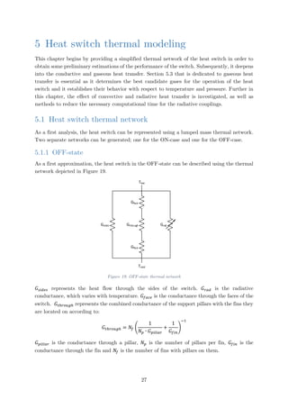
![Figure 16: Units temperature profile (worst hot, no switch)
Figure 17 shows the temperature profile of the +Z panel, which accommodates the batteries,
for the worst cold case in the absence of the heat switch. In order to maintain the temperature
of the batteries above the minimum temperature of 14o
C, an average heating power of 30.19
W and 34.07 W needs to be supplied to Battery 1 and Battery 2 respectively, for a total of
64.26 W. This is achieved by supplying a power of 50 W to Battery 1 and 60 W to Battery 2
if their individual temperature drops below 14.5o
C. The difference in the power is due to the
fact that only one battery is operating and thus dissipating power, while the second one exists
for redundancy purposes.
Figure 17: +Z panel temperature profile (Worst cold, no switch)
10
15
20
25
30
35
40
0 10,000 20,000 30,000 40,000 50,000 60,000
Temperature[oC]
Time [s]
COMS
BAT1
BAT2
PCDU
SBT1
SBT2
WDE
MMFU
ICU1
ICU2
GPS
OBC
RIU
13
14
14
14
14
14
15
15
15
0 10,000 20,000 30,000 40,000 50,000 60,000 70,000
Temperature[oC]
Time [s]
COMS
BAT1
BAT2
25](https://image.slidesharecdn.com/ab16c9ba-74cc-44a4-aa76-d5a97c25dce8-160912051601/85/AE5810-Thesis-38-320.jpg)
![Table 9: 10x10 cm2
OFF-case thermal conductances
Label 𝒍𝒍 [𝒎𝒎𝒎𝒎] 𝑨𝑨 [𝒎𝒎𝒎𝒎𝟐𝟐
] Quantity
Conductance
[W/K]
𝐺𝐺𝑠𝑠𝑠𝑠𝑠𝑠𝑠𝑠𝑠𝑠1 11.14 50 1 0.0301
𝐺𝐺𝑠𝑠𝑠𝑠𝑠𝑠𝑠𝑠𝑠𝑠2 21.24 50 3 0.0158
𝐺𝐺𝑓𝑓𝑓𝑓𝑓𝑓𝑓𝑓 0.7 10,000 2 95.7143
𝐺𝐺𝑝𝑝𝑝𝑝𝑝𝑝𝑝𝑝𝑝𝑝𝑝𝑝 0.2 0.0491 𝑁𝑁𝑝𝑝 = 8 0.00164
𝐺𝐺𝑓𝑓𝑓𝑓𝑓𝑓 1.6 25 𝑁𝑁𝑓𝑓 = 8 0.1047
𝐺𝐺𝑐𝑐𝑐𝑐𝑐𝑐𝑐𝑐 - - - 0.1919
For small temperature differences between two radiating surfaces the non-linear radiative
conductance can be transformed into a linear conductance using the Taylor-series expansion
[23].
𝐺𝐺𝑅𝑅
′
= 4𝜎𝜎𝑇𝑇�3
𝐺𝐺𝑅𝑅 (5.1-1)
Assuming an average temperature of 288 K between the hot and cold side and linearizing the
radiative conductance, 𝐺𝐺𝑟𝑟𝑟𝑟𝑟𝑟,𝑙𝑙𝑙𝑙𝑙𝑙𝑙𝑙𝑙𝑙𝑙𝑙𝑙𝑙𝑙𝑙𝑙𝑙𝑙𝑙 = 0.0758 𝑊𝑊/𝐾𝐾. Thus, the total OFF-conductance is
𝐺𝐺𝑂𝑂𝑂𝑂𝑂𝑂,𝑡𝑡𝑡𝑡𝑡𝑡𝑡𝑡𝑡𝑡 = 0.268 𝑊𝑊/𝐾𝐾. For the estimation of the radiative conductance, refer to section 5.5.1.
Table 10: 20x20 cm2
OFF-case thermal conductances
Label 𝒍𝒍 [𝒎𝒎𝒎𝒎] 𝑨𝑨 [𝒎𝒎𝒎𝒎𝟐𝟐
] Quantity
Conductance
[W/K]
𝐺𝐺𝑠𝑠𝑠𝑠𝑠𝑠𝑠𝑠𝑠𝑠1 9.94 80 1 0.0539
𝐺𝐺𝑠𝑠𝑠𝑠𝑠𝑠𝑠𝑠𝑠𝑠2 19.29 80 3 0.0278
𝐺𝐺𝑓𝑓𝑓𝑓𝑓𝑓𝑓𝑓 0.7 40,000 2 382.8571
𝐺𝐺𝑝𝑝𝑝𝑝𝑝𝑝𝑝𝑝𝑝𝑝𝑝𝑝 0.2 0.0866 𝑁𝑁𝑝𝑝 = 16 0.00290
𝐺𝐺𝑓𝑓𝑓𝑓𝑓𝑓 0.6 50 𝑁𝑁𝑓𝑓 = 16 0.5583
𝐺𝐺𝑐𝑐𝑐𝑐𝑐𝑐𝑐𝑐 - - - 0.6854
Assuming an average temperature of 288 K between the hot and cold side and linearizing the
radiative conductance, 𝐺𝐺𝑟𝑟𝑟𝑟𝑟𝑟,𝑙𝑙𝑙𝑙𝑙𝑙𝑙𝑙𝑙𝑙𝑙𝑙𝑙𝑙𝑙𝑙𝑙𝑙𝑙𝑙 = 0.1325 𝑊𝑊/𝐾𝐾. Thus, the total OFF-conductance is
𝐺𝐺𝑂𝑂𝑂𝑂𝑂𝑂,𝑡𝑡𝑡𝑡𝑡𝑡𝑡𝑡𝑡𝑡 = 0.818 𝑊𝑊/𝐾𝐾.
Eventually, in the OFF-state the switch can be represented with two isothermal nodes that
are coupled together with one radiative and one conductive conductance (combination of all
other conductive conductances) in parallel. The equation to describe this heat exchange is:
𝑄𝑄 = 𝐺𝐺𝑐𝑐𝑐𝑐𝑐𝑐𝑐𝑐(𝑇𝑇ℎ − 𝑇𝑇𝑐𝑐) + 𝐺𝐺𝑟𝑟𝑟𝑟𝑟𝑟(𝜎𝜎𝛵𝛵ℎ
4
− 𝜎𝜎𝛵𝛵𝑐𝑐
4
) (5.1-2)
28](https://image.slidesharecdn.com/ab16c9ba-74cc-44a4-aa76-d5a97c25dce8-160912051601/85/AE5810-Thesis-41-320.jpg)
![through an iterative process that involved the improvement of the FEM building up to the
test setup. Eventually, in the thermal simulation, the baseplate of the vacuum chamber is held
at a constant temperature 𝑇𝑇𝑏𝑏𝑏𝑏𝑏𝑏𝑏𝑏𝑏𝑏𝑏𝑏𝑏𝑏𝑏𝑏𝑏𝑏 = 20℃, while a constant heat load is applied on the top
face of an aluminium plate. For more information on the test setup, please refer to Chapter 7.
In the absence of other thermal couplings, radiative or conductive, 𝐺𝐺𝑐𝑐𝑐𝑐𝑐𝑐𝑐𝑐 can be calculated
using the temperature difference between the hot and cold side of the switch as:
𝐺𝐺𝑐𝑐𝑜𝑜𝑜𝑜𝑜𝑜 =
𝑄𝑄
𝑇𝑇ℎ − 𝑇𝑇𝑐𝑐
(5.2-1)
Table 11 summarizes the obtained results for the conductive conductances for the second and
third prototype of the heat switch.
Table 11: Conductive conductances of different prototypes
Prototyp
e
Area Material
# of
pillar
s
Conductive
Conductance
[W/o
C]
Conductive
heat transfer
coefficient
[W/m2
K]
Second 10 cm x 10 cm Ti-6Al-4V 64 0.1465 14.65
Second 10 cm x 10 cm Inconel 718® 64 0.2345 23.45
Third 20 cm x 20 cm Ti-6Al-4V 256 0.4084 10.21
5.3 Gaseous heat transfer
Knudsen number is a dimensionless number used particularly in the microscale in order to
determine whether the continuum assumption is respected. Knudsen number expresses the
ratio of the mean free path to the characteristic length of the system. The mean free path
expresses the probability distance a fluid particle travels before undergoing collision with
another fluid particle [24]. Assuming the molecules to be rigid and spherical, the mean free
path for a single component ideal-gas can be approximated as [15]:
𝜆𝜆 =
𝑘𝑘𝐵𝐵 𝑇𝑇
𝜋𝜋𝑑𝑑2√2𝑝𝑝
(5.3-1)
𝑘𝑘𝐵𝐵 = 1.38065 ∙ 10−23
[
𝐽𝐽
𝐾𝐾
] is the Boltzmann constant, 𝑇𝑇 is the gas temperature in Kelvin, 𝑑𝑑 is
the effective molecular diameter and 𝑝𝑝 is the gas pressure in Pascals.
The Knudsen number is expressed as [25]:
𝐾𝐾𝐾𝐾 =
𝑚𝑚𝑚𝑚𝑚𝑚𝑚𝑚 𝑓𝑓𝑓𝑓𝑓𝑓𝑓𝑓 𝑝𝑝𝑝𝑝𝑝𝑝ℎ
𝑐𝑐ℎ𝑎𝑎𝑎𝑎𝑎𝑎𝑎𝑎𝑎𝑎𝑎𝑎𝑎𝑎𝑎𝑎𝑎𝑎𝑎𝑎𝑎𝑎𝑎𝑎 𝑙𝑙𝑙𝑙𝑙𝑙𝑙𝑙𝑙𝑙ℎ
=
𝜆𝜆
𝐿𝐿
(5.3-2)
If 𝐾𝐾𝐾𝐾 < 0.01, the interfluid particle collisions dominate and the system is in the continuum
regime. In the continuum regime, the gas particles collide with each other and the heat is
31](https://image.slidesharecdn.com/ab16c9ba-74cc-44a4-aa76-d5a97c25dce8-160912051601/85/AE5810-Thesis-44-320.jpg)
![transferred in the most efficient way through the gas. Further increase in pressure does not
affect the thermal conductivity of the gas.
If 𝐾𝐾𝐾𝐾 > 10, the continuum assumption breaks down and the system is in the molecular regime.
In this case, the probability of the fluid particles colliding with the surrounding walls is
significantly higher than colliding with each other.
For the intermediate range 0.01 < 𝐾𝐾𝐾𝐾 < 10, heat conduction takes place in the transition
regime. The temperature jump approximation, which is an averaging of the two extreme
regimes, can be used in order to estimate the thermal conductivity of the gas.
It should be noted that these limits are approximate and can vary depending on the gas and
the solid it comes in contact with. For more information, please refer to section 5.3.4.
The profile of the thermal conductivity of a gas across the three different regimes is similar to
the one in Figure 22. The figure shows the variation of thermal conductivity of Argon gas
occupying spacing between two Tungsten plates separated by 1 μm, at 300 K.
Figure 22: Variation of thermal conductivity of Argon [24]
5.3.1 Continuum regime thermal conductivity
In the continuum regime, the thermal conductivity of a gas can be estimated using the Prandtl
number. The Prandtl number is dimensionless and expresses the ratio of the viscous to the
thermal diffusion rate [6].
𝑃𝑃𝑃𝑃 =
𝐶𝐶𝑝𝑝 𝜇𝜇
𝑘𝑘
=
9𝛾𝛾 − 5
4𝛾𝛾
(5.3-3)
𝐶𝐶𝑝𝑝 [
𝐽𝐽
𝑘𝑘𝑘𝑘∙𝐾𝐾
] is the specific heat, 𝜇𝜇 [𝑃𝑃𝑃𝑃 ∙ 𝑠𝑠] is the dynamic viscosity and 𝑘𝑘[
𝑊𝑊
𝑚𝑚∙𝐾𝐾
] is the thermal
conductivity of the gas.
The dynamic viscosity can be estimated using the average molecular speed [15]:
32](https://image.slidesharecdn.com/ab16c9ba-74cc-44a4-aa76-d5a97c25dce8-160912051601/85/AE5810-Thesis-45-320.jpg)
![𝜇𝜇 =
1
2
𝜌𝜌𝐶𝐶𝜆𝜆 (5.3-4)
The average molecular speed is given by Maxwell’s equilibrium formula [15]:
𝐶𝐶 = �
8𝑁𝑁𝐴𝐴 𝑘𝑘𝐵𝐵 𝑇𝑇
𝜋𝜋𝜋𝜋
(5.3-5)
𝑁𝑁𝐴𝐴 = 6.022 ∙ 1023 [𝑚𝑚𝑚𝑚𝑙𝑙−1] is the Avogadro number and 𝑀𝑀 is the gram molecular mass.
From thermodynamics we know:
𝐶𝐶𝑝𝑝 = 𝛾𝛾𝐶𝐶𝑣𝑣 = 𝛾𝛾
𝑓𝑓𝑓𝑓
2
(5.3-6)
Where, 𝑅𝑅 = 8.314 [
𝐽𝐽
𝑚𝑚𝑚𝑚𝑚𝑚∙𝐾𝐾
] is the universal gas constant and 𝑓𝑓 expresses the number of degrees
of freedom of the gas. For a monoatomic gas 𝑓𝑓 = 3, and for a diatomic gas 𝑓𝑓 = 5.
The number of degrees of freedom for linear and non-linear molecules are given by equations
(5.3-7) and (5.3-8) respectively, where is 𝑛𝑛 the number of atoms in the molecules:
𝑓𝑓 = 3𝑛𝑛 − 5 (5.3-7)
𝑓𝑓 = 3𝑛𝑛 − 6 (5.3-8)
Combining equations (5.3-1) to (5.3-6), the thermal conductivity of a gas in the continuum
regime can be approximated with equation (5.3-9). From this equation, it is clear that the
thermal conductivity is independent of the gas pressure. The only environmental condition
affecting the thermal conductivity is the gas temperature.
𝑘𝑘 =
9𝛾𝛾 − 5
8
𝑓𝑓𝑓𝑓
𝑁𝑁𝐴𝐴 𝜋𝜋𝑑𝑑2
�
𝑅𝑅𝑅𝑅
𝜋𝜋𝜋𝜋
(5.3-9)
For the ON-state of the heat switch, the thermal conductivity of the gas shall be as high as
possible. Thus, this equation can be used in order to determine the best candidates for the
working fluid inside the heat switch gap. From equation (5.3-9), it is clear that a gas with a
minimal molecular mass and diameter along with a high number of degrees of freedom and
specific heat ratio is required.
Summarizes the approximated thermal conductivities in descending order for several of the
gases that were taken into account at 300 K. All properties except for k were obtained from
references [15] and [24].
33](https://image.slidesharecdn.com/ab16c9ba-74cc-44a4-aa76-d5a97c25dce8-160912051601/85/AE5810-Thesis-46-320.jpg)
![Table 12: Gas thermal conductivities at 300 K
Gas d [Å] f γ M [kg/kmol] k [W/mK]
H2 (Hydrogen) 2.74 5 1.408 2.016 0.1761
He (Helium) 2.18 3 1.667 4.003 0.1545
Ne (Neon) 2.59 3 1.667 20.18 0.0487
N2 (Nitrogen) 3.75 5 1.401 28.01 0.0250
Air 3.64 5 1.401 28.96 0.0250
CH4 (Methane) 4.14 5 1.320 16.04 0.0246
CO2 (Carbon dioxide) 3.91 4 1.288 44.01 0.0157
Consequently, the best candidates are by far Hydrogen and Helium with Neon as another
option. However, because of ESTEC safety constraints, experiments with Hydrogen are not
allowed in the facilities. Consequently, Hydrogen can be used only as a reference for future
testing at a different facility. Only Helium and Neon will be used throughout the experiments.
After the best candidates are identified, more accurate formulations can be used in order to
determine the thermal conductivity of the three gases within a certain temperature range. For
monoatomic gases, such as Helium and Neon, the thermal conductivity can be estimated as
[15]:
𝑘𝑘 =
0.083228
𝑑𝑑2 𝛺𝛺𝑘𝑘
�
𝑇𝑇
𝑀𝑀
(5.3-10)
For polyatomic gases, such as Hydrogen, a variation of equation (5.3-3) can be used to estimate
the thermal conductivity:
𝑘𝑘 =
9𝛾𝛾 − 5
4𝛾𝛾
𝜇𝜇𝐶𝐶𝑝𝑝 (5.3-11)
The dynamic viscosity is predicted as follows [15]:
𝜇𝜇 = 2.6693 ∙ 10−6 √𝑀𝑀 ∙ 𝑇𝑇
𝜎𝜎2 𝛺𝛺𝜇𝜇
(5.3-12)
The dynamic viscosity is in Pa∙s, the thermal conductivity in W/m∙K, the molecular diameter
in Å. 𝛺𝛺𝜇𝜇 and 𝛺𝛺𝑘𝑘 are collision integrals for the viscosity and thermal conductivity obtained
from Table 27 and Table 28 in Appendix A. The equations are derived using the Lennard-
Jones intermolecular potential. The obtained results at 300 K were almost identical with
tabulated data for Helium and Neon, with a deviation of less than 1%. In the case of Hydrogen,
the thermal conductivity was under-predicted by 5%, which was expected according to
reference [26]. Appendix D includes graphical data of the experimental values for the thermal
conductivity, density and heat capacity of the gases with respect to temperature.
34](https://image.slidesharecdn.com/ab16c9ba-74cc-44a4-aa76-d5a97c25dce8-160912051601/85/AE5810-Thesis-47-320.jpg)
![5.3.2 Free molecular regime thermal conductivity
In the free molecular regime, the thermal conductivity of a gas can be estimated using equation
(5.3-13) [24].
𝑘𝑘𝐹𝐹𝐹𝐹 =
𝑃𝑃 �𝐶𝐶𝑣𝑣,𝑚𝑚 +
𝑅𝑅
2�
1
𝛽𝛽1
+
1
𝛽𝛽2
− 1
1
√2𝜋𝜋𝜋𝜋𝜋𝜋𝑇𝑇′
(5.3-13)
𝐶𝐶𝑣𝑣,𝑚𝑚 is the molar heat capacity of the gas at constant volume, 𝛽𝛽1, 𝛽𝛽2 are the accommodation
coefficients of the surfaces. 𝑇𝑇′
is defined as [27]:
1
√𝑇𝑇′
=
1
2
�
1
�𝑇𝑇1
′
+
1
�𝑇𝑇2
′
� (5.3-14)
𝑇𝑇1
′
=
𝛽𝛽1 𝑇𝑇1 + 𝛽𝛽2(1 − 𝛽𝛽1)𝑇𝑇2
𝛽𝛽1 + 𝛽𝛽2 − 𝛽𝛽1 𝛽𝛽2
(5.3-15)
𝑇𝑇2
′
=
𝛽𝛽2 𝑇𝑇2 + 𝛽𝛽1(1 − 𝛽𝛽2)𝑇𝑇1
𝛽𝛽1 + 𝛽𝛽2 − 𝛽𝛽1 𝛽𝛽2
(5.3-16)
The accommodation coefficient is a physical quantity that varies between 0 and 1 and
characterizes the behavior of gas molecules colliding with a solid body. It is dependent on the
surface and the composition of the gas [28]. The accommodation coefficient for the gases can
be estimated using the following experimental correlation [29]:
𝛽𝛽 = ��
𝑀𝑀𝑔𝑔
∗
𝐶𝐶1 + 𝑀𝑀𝑔𝑔
∗� 𝑒𝑒
�𝐶𝐶0�
𝑇𝑇𝑠𝑠−𝑇𝑇0
𝑇𝑇0
��
� + �
2.4𝜇𝜇
(1 + 𝜇𝜇)2
∙ �1 − 𝑒𝑒
�𝐶𝐶0�
𝑇𝑇𝑠𝑠−𝑇𝑇0
𝑇𝑇0
��
�� (5.3-17)
𝐶𝐶0 = −0.57, 𝐶𝐶1 = 6.8, 𝑇𝑇0 = 273 𝐾𝐾, 𝑇𝑇𝑠𝑠 is the surface temperature, 𝑀𝑀𝑔𝑔
∗
= 𝑀𝑀𝑔𝑔 for monoatomic
gases and 𝑀𝑀𝑔𝑔
∗
= 1.4𝑀𝑀𝑔𝑔 for diatomic or polyatomic gases, where 𝑀𝑀𝑔𝑔 is the gas molecular mass.
𝜇𝜇 =
𝑀𝑀𝑔𝑔
𝑀𝑀𝑠𝑠
is the ratio of the molecular mass of the gas to the molecular mass of the solid.
In this case we could assume 𝑇𝑇𝑠𝑠 = 𝑇𝑇′
from equation (5.3-14). Additionally, because Ti-6Al-4V
and Inconel 718® are alloys, a weighted average of their molecular masses of the constituent
molecules was used. For their chemical composition, please refer to Appendix F. Table 13
summarizes the obtained results for the accommodation coefficient of three gases with the two
alloys, when 𝑇𝑇1 = 293 𝐾𝐾 and 𝑇𝑇2 = 318 𝐾𝐾. This gradient is an initial estimation for the OFF-
case at a baseplate temperature of 20o
C.
35](https://image.slidesharecdn.com/ab16c9ba-74cc-44a4-aa76-d5a97c25dce8-160912051601/85/AE5810-Thesis-48-320.jpg)
![Table 13: Gases accommodation coefficients
Gas Ti-6Al-4V Inconel 718®
Hydrogen 0.280 0.279
Helium 0.358 0.237
Neon 0.732 0.349
5.3.3 Transition regime thermal conductivity
The thermal conductivity of a monoatomic gas in the transition regime can be modeled using
the temperature jump approximation according to [28]:
𝑘𝑘𝑇𝑇𝑇𝑇 = 𝑘𝑘𝐹𝐹𝐹𝐹 �1 +
4
15
𝐵𝐵
𝐾𝐾𝐾𝐾
𝛽𝛽1 𝛽𝛽2
𝛽𝛽1 + 𝛽𝛽2 − 𝛽𝛽1 𝛽𝛽2
�
−1
(5.3-18)
𝐵𝐵 = 1.0 for monoatomic gases, 𝐵𝐵 = 45 38⁄ for polyatomic gases.
Figure 23 provides a plot of the thermal conductivity of Helium, Neon and Hydrogen across
the transition regime. Below 0.1 mbar, the thermal conductivity is in the order of 10-4
W/m∙K
and consequently the conduction through the gas is insignificant. Helium reaches a plateau at
a pressure of around 1000 mbar, Neon around 200 mbar and Hydrogen around 700 mbar.
Figure 23: Gas thermal conductivity in the transition regime
Normally, a slight jump in the thermal conductivity of a gas is observed at the continuum
regime boundary. Such a jump can be seen in Figure 22. This jump explains the slightly smaller
value of the estimated thermal conductivity at the continuum regime boundary compared to
the experimental values in the continuum regime.
5.3.4 Regime pressure limits
The pressure that corresponds to the entry in the continuum regime and the free molecular
regime had to be determined for all the gases in preparation of the test procedure. Combining
0
0.02
0.04
0.06
0.08
0.1
0.12
0.14
0.16
0.18
0.01 0.1 1 10 100 1000
Thermalconductivity[W/m∙K]
Pressure [mbar]
Helium Neon Hydrogen
36](https://image.slidesharecdn.com/ab16c9ba-74cc-44a4-aa76-d5a97c25dce8-160912051601/85/AE5810-Thesis-49-320.jpg)
![equations (5.3-2) and (5.3-1) and applying the nominal regime limits, the respective pressure
can be obtained. For pairs of fluid particle and solid surface with small accommodation
coefficients, such as Helium with Titanium, the transition to the continuum regime occurs at
a smaller Knudsen number, i.e. at a higher pressure [24]. Figure 24 provides a correlation
between the accommodation coefficient and the Knudsen number for the different regimes.
Figure 24: Classification of free-molecular, transition, and continuum regimes for heat conduction across a gas
confined between parallel plates [24]
Table 14 summarizes the estimated pressure limits for Hydrogen, Helium and Neon at 20o
C
for the characteristic length of 0.2 mm.
Table 14: Regime pressure limits
Regime
H2 He Ne
Kn P [mbar] Kn P [mbar] Kn P [mbar]
Molecular >12.50 <0.0485 >16.67 <0.0575 >50 <0.0136
Continuum <9.091E-04 >667 <1.0E-03 >958 <5.0E-03 >136
5.4 Convective heat transfer
In addition to the conduction through the gas, the free convection effects needed to be
evaluated. The natural convection heat transfer mechanism relies on buoyancy forces.
Consequently, in the absence of gravity no convection occurs. However, since this is a ground
test, the extent of the convection effects have to be determined.
The natural convection coefficient ℎ is estimated using Rayleigh and Nusselt numbers.
Rayleigh number is the product of the Prandtl number and the Grashof number. Grashof
number expresses the relationship between buoyancy and viscosity within a fluid. For free
convection inside enclosures, the Rayleigh number is determined as [6]:
𝑅𝑅𝑅𝑅𝐿𝐿 =
𝑔𝑔𝛽𝛽(𝑇𝑇1 − 𝑇𝑇2)𝐿𝐿𝑐𝑐
3
𝜈𝜈2
𝑃𝑃𝑃𝑃 (5.4-1)
37](https://image.slidesharecdn.com/ab16c9ba-74cc-44a4-aa76-d5a97c25dce8-160912051601/85/AE5810-Thesis-50-320.jpg)
![𝑔𝑔 is the gravitational acceleration, 𝛽𝛽 is the coefficient of volume expansion (1/𝑇𝑇 for ideal
gases), 𝐿𝐿𝑐𝑐 is the distance between the hot and cold surfaces and 𝜈𝜈 is the kinematic viscosity of
the fluid. All the fluid properties are evaluated at the average surface temperature 𝑇𝑇� =
𝑇𝑇1+𝑇𝑇2
2
.
In an enclosure, a fluid behaves like a fluid whose thermal conductivity is 𝑘𝑘 ∙ 𝑁𝑁𝑁𝑁 as a results
of convection currents. This value is defined as the effective thermal conductivity [6]:
𝑘𝑘𝑒𝑒𝑒𝑒𝑒𝑒 = 𝑘𝑘 ∙ 𝑁𝑁𝑁𝑁 (5.4-2)
𝑁𝑁𝑁𝑁 =
ℎ𝐿𝐿
𝑘𝑘
(5.4-3)
When the hotter plate is at the top, as shown in Figure 25a, no convection currents develop
in the enclosure, since the lighter fluid is always on top of the heavier fluid. Consequently, the
heat transfer occurs only by conduction and 𝑁𝑁𝑁𝑁 = 1. Thus, the effective thermal conductivity
becomes the thermal conductivity of the fluid [6]. This is the case for the heat transfer between
faces 1-2 and 5-6 in Figure 131 and Figure 132 of Appendix E.
Figure 25: Convective currents in a horizontal
enclosure [6]
Figure 26: A vertical rectangular enclosure with
isothermal surfaces [6]
However, this is not the case for the vertical plate configuration of faces 3-4. In this case the
natural convection coefficient can be approximated using correlations of the Nusselt number
with the Rayleigh number for vertical rectangular enclosures [6].
𝑁𝑁𝑁𝑁 = 0.22 �
𝑃𝑃𝑃𝑃
0.2 + 𝑃𝑃𝑃𝑃
𝑅𝑅𝑎𝑎𝐿𝐿�
0.28
�
𝐻𝐻
𝐿𝐿
�
−0.25
(5.4-4)
This correlation is valid for any Prandtl number, 2 <
𝐻𝐻
𝐿𝐿
< 10, and 𝑅𝑅𝑎𝑎𝐿𝐿 < 1010
. Assuming 𝑇𝑇1 =
295 𝐾𝐾 and 𝑇𝑇2 = 285 𝐾𝐾 and taking the Helium properties at 𝑇𝑇� = 290 𝐾𝐾 and a pressure of 2 bar,
𝑘𝑘 = 0.1524 𝑊𝑊/𝑚𝑚 ∙ 𝐾𝐾, 𝜈𝜈 = 5.872 ∙ 10−5
𝑚𝑚2
/𝑠𝑠, 𝐶𝐶𝑝𝑝 = 5193 J/kg ∙ K, 𝑃𝑃𝑃𝑃 = 0.6635. For the given
characteristic length of 0.2 mm, this results in 𝑅𝑅𝑎𝑎𝐿𝐿 = 5.2 ∙ 10−4
. For the second and third
prototype �
𝐻𝐻
𝐿𝐿
�
2𝑛𝑛𝑛𝑛
= 8 and �
𝐻𝐻
𝐿𝐿
�
3𝑟𝑟𝑟𝑟
= 3 respectively, we obtain (𝑁𝑁𝑁𝑁)2𝑛𝑛𝑛𝑛 = 0.015 and (𝑁𝑁𝑁𝑁)3𝑟𝑟𝑟𝑟 =
0.019. These values are below the minimum value of 1 for the Nusselt number. Consequently,
no convection occurs in this case either. The order of magnitude does not change with
38](https://image.slidesharecdn.com/ab16c9ba-74cc-44a4-aa76-d5a97c25dce8-160912051601/85/AE5810-Thesis-51-320.jpg)
![temperature, pressure and gas. Therefore, it is safe to assume that convection does not occur
in any case.
5.5 Radiative heat transfer
The effects of radiative heat transfer through the gap needed to be evaluated. In the thermal
model, a hemispherical emissivity of 0.57 and 0.48 was used for the second and third prototype
respectively. For more information on the origin of these values, please refer to section 6.1.
5.5.1 Radiative coupling through gap
A simplification of the system would be to consider the gap to consist of infinitely long parallel
plates. This is because the length of the fins is two to three orders of magnitude larger than
the gap. In this case the view factor between the plates is 1 and the radiative heat transfer
can be estimated according to the configuration shown in Figure 27.
Figure 27: Infinitely large parallel plates radiation heat exchange [6]
The effective emissivity is expressed by the equation:
𝜀𝜀𝑒𝑒𝑒𝑒𝑒𝑒 =
1
1
𝜀𝜀1
+
1
𝜀𝜀2
− 1
(5.5-1)
The effective emissivity for the second prototype is 0.3986. The second prototype has a total
internal gap area of 0.044 m2
. With an emissivity of 0.57, the radiative conductance is:
𝐺𝐺𝑟𝑟𝑟𝑟𝑟𝑟 = 𝜀𝜀𝑒𝑒𝑒𝑒𝑒𝑒 ∙ 𝐴𝐴 = 0.01754 𝑚𝑚2
For a more detailed analysis, the two parallel strip configuration from Appendix E can be used
in order to calculate the view factors for one fin. The resulting radiative conductance per fin
is 1.1522∙10-4
m2
. When multiplied with the total number of fins, the total radiative
conductance of the switch is 0.01279 m2
. This results in a difference of 37.1%.
Using the infinitely long parallel plates assumption, the third prototype has an effective
emissivity of 0.3158 and a total internal gap area of 0.0930 m2
. In this case, the radiative
conductance is:
𝐺𝐺𝑟𝑟𝑟𝑟𝑟𝑟 = 𝜀𝜀𝑒𝑒𝑒𝑒𝑒𝑒 ∙ 𝐴𝐴 = 0.02937 𝑚𝑚2
The analytical view factor approach, similar to the second prototype results in a radiative
conductance per fin of 1.0090∙10-4
m2
. When multiplied with the total number of fins, the total
39](https://image.slidesharecdn.com/ab16c9ba-74cc-44a4-aa76-d5a97c25dce8-160912051601/85/AE5810-Thesis-52-320.jpg)
![radiative resistance of the switch is 0.02230 m2
, which represents a 31.7% difference with the
infinitely large parallel plate configuration.
Because of the large number of elements in the FEM, calculating the actual view factors for
all fins would be computationally very expensive. Consequently, the effective emissivity can
be adjusted in order to obtain the same radiative conductance. A dummy case was generated
using only two fins per side to reduce the computational time. A detailed radiation enclosure
was generated, using the Monte Carlo method by firing 5000 rays per element. The results of
this simulation were used to derive a simplified radiative model. Through an iterative process
the effective emissivity of the gap radiation was adjusted. Eventually, an effective emissivity
of 0.318 for the second prototype and 0.263 for the third prototype resulted in deviations of
temperature and radiative heat fluxes of less than 1% when compared to the Monte Carlo
method. The resulting total radiative conductance is 0.01399 m2
and 0.02446 m2
for the second
and third prototype respectively. The difference with the analytical view factor approach can
be attributed to the reflections on the surfaces, which were not taken into account in the latter.
Additionally, in the GMM the fins are discretized into smaller surfaces providing higher
accuracy.
5.5.2 Gas radiation
For transparent media, the radiation that propagates through them remains unchanged.
Though, certain gases absorb and emit radiation in various wavelength spectra, the absorption
bands. This concept is used in spectroscopy in order to identify the gases present in a planet’s
atmosphere. The emissivity of the gases is a function of the temperature, the partial and total
pressure, as well as the thickness of the gas. Gases that exhibit such behavior are CO, NO,
CO2, SO2 and water [7]. Among these gases, only CO2 had been taken into account as a
potential candidate for the heat switch, but it was discarded due to its low thermal
conductivity. Hydrogen and noble gases do not exhibit gas radiation properties and therefore
no further analysis was required on this topic.
5.6 Summary
The main thermal concepts behind the function of the heat switch are the conductive heat
transfer through the solid material, the gaseous heat transfer with respect to pressure and
temperature and the radiative heat transfer between the hot and cold side of the heat switch.
Reduced thermal models and FEM were produced to simulate the behavior of the switch based
on these concepts. Convective heat transfer and gas radiation were also investigated. Though
their effect on the behavior of the heat switch was proved to be of no importance and thus,
no further attention is paid to them.
40](https://image.slidesharecdn.com/ab16c9ba-74cc-44a4-aa76-d5a97c25dce8-160912051601/85/AE5810-Thesis-53-320.jpg)
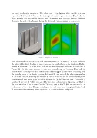
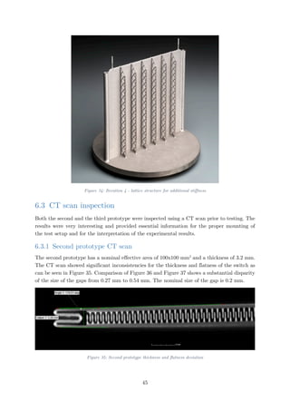
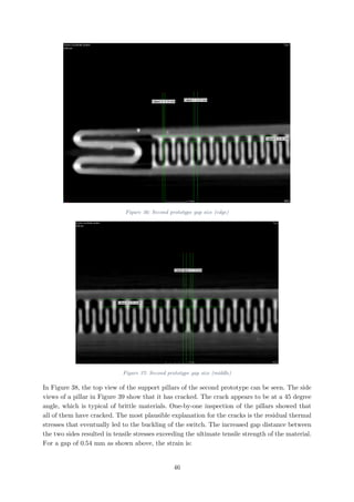
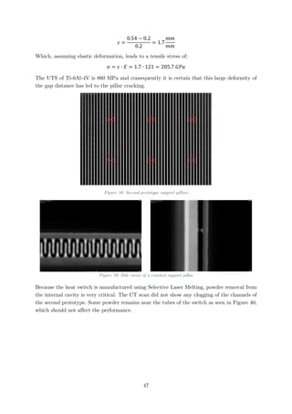
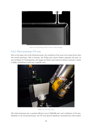
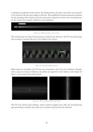
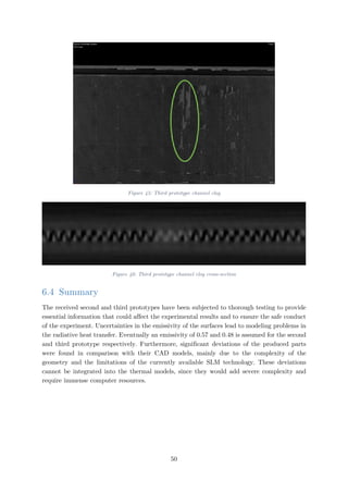
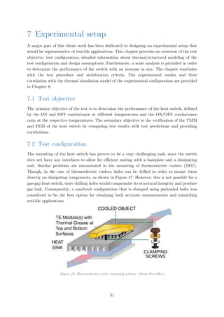
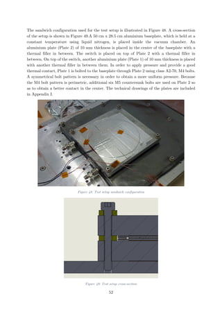
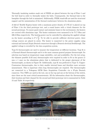
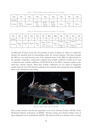
![The cold plate and shroud temperature range is -170o
C to +80o
C. The vacuum limit is less
than 5∙10-4
mbar.
The inlet and outlet of the switch have an outer diameter of 3.18 mm (1/8 inch) and are
connected to stainless steel tubing using straight union Swagelok® fittings made of stainless
steel. According to manufacturer’s specification, the tubing shall be softer than the fitting. Ti-
6Al-4V has a hardness of HRB 712
, while SS of HRB 793
, satisfying this requirement.
Additionally, in vacuum and hence in the absence of an electrolyte, no galvanic corrosion is
expected to occur externally. Internally, Helium and Neon are used, which are inert gases and
do not contribute to corrosion. Because of the CTE mismatch between Ti-6Al-4V and SS,
extreme care shall be taken not to have significant temperature gradients at the interface.
Such gradients induce thermal stresses that can damage the prototype and the test equipment.
The heat switch is pressurized using either Helium or Neon tank depending on the test case.
A pressure regulator is attached to the tanks and a precision valve is used to control the inlet
flow when pressurizing the switch. The maximum pressure shall not exceed 5.33 bar, which is
dictated by the overpressure limit of the pressure transducer used. The pressure transducer
that measures the internal pressure of the heat switch is the 722B Baratron® Compact
Absolute Capacitance Manometer from MKS. The full scale pressure range is 1 to 2000 Torr
with a reading accuracy of ±0.5%, including non-linearity, hysteresis and non-repeatability.
The pressure reading is provided as a measured voltage from the pressure transducer. The
nominal curve is given by 𝑃𝑃 = 0.2666 ∙ 𝑉𝑉 [𝑏𝑏𝑏𝑏𝑏𝑏]. The curve of pressure against measured voltage
for the calibrated pressure transducer is shown in Figure 52. Because the pressure sensor is
impossible to be placed inside the heat switch, it is placed at the outlet tubing just outside of
the vacuum chamber. A rotary pump is placed at the end of the outlet tubing. A schematic of
the pressure handling system is show in Figure 53.
Figure 52: Pressure sensor calibration curve
2
From MatWeb: Titanium Ti-6Al-4V (Grade 5), STA
3
From MatWeb: 316 Stainless Steel, annealed sheet
y = 0.265840x - 0.023305
0.0
0.5
1.0
1.5
2.0
2.5
3.0
0.0 2.0 4.0 6.0 8.0 10.0 12.0
Pressure[bar]
Measured voltage [V]
55](https://image.slidesharecdn.com/ab16c9ba-74cc-44a4-aa76-d5a97c25dce8-160912051601/85/AE5810-Thesis-68-320.jpg)
![Figure 53: Pressure handling system schematic
7.3 Test configuration leak inspection
A leak inspection was conducted on the heat switch and the test assembly to prevent
significant gas losses and contamination. The maximum allowable leakage rate can be
determined using equation (7.3-1) [25].
𝑄𝑄𝐿𝐿 =
𝛥𝛥𝑝𝑝 ∙ 𝑉𝑉
𝛥𝛥𝑡𝑡
(7.3-1)
where 𝛥𝛥𝑝𝑝 is the allowable pressure change, 𝛥𝛥𝑡𝑡 is the measurement period and 𝑉𝑉 is the volume.
For the given test, it was deemed appropriate to not allow for a pressure drop of more than
10 mbar over 24 hours. This is to ensure the gas remains in the continuum regime over the
entire test process that lasts no more than a day for the ON-case. The total internal volume
of the test setup, including the heat switch and the tubing is 0.0280 L for the 10x10 cm2
and
0.0223 L for the 20x20 cm2
heat switch. Consequently, the allowable leakage rate is 3.2∙10-6
and 2.6∙10-6
mbar∙L/s respectively. The helium leak detector (Mass Spectrometer Leak
Detector) measured a maximum leakage rate in the order 10-7
in the tubing. However, for the
second prototype, a significant leakage of 4.0∙10-6
mbar∙L/s was detected around the sides of
the switch. Unfortunately, this leakage cannot be controlled since it stems directly from the
solid part. Such leakage could be the result of cracks or of the porosity of the 3D-printed
titanium heat switch that could potentially allow the tiny molecules of Helium to penetrate
through the solid. For the third prototype, the maximum leakage rate was measured at 3.7
∙10-6
mbar∙L/s. It should be noted that the leak test was conducted at room temperature.
The effects of the materials contraction and expansion due to temperature variation are not
known. Since stainless steel tube fittings are placed on Ti-6Al-4V parts, it is possible to
experience leakage, especially when exposed to a cold environment due to the difference in the
material CTE.
56](https://image.slidesharecdn.com/ab16c9ba-74cc-44a4-aa76-d5a97c25dce8-160912051601/85/AE5810-Thesis-69-320.jpg)
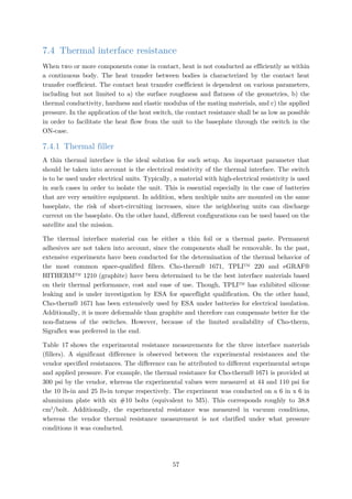
![Table 17: Fillers thermal resistance4
Thermal Filler
Electrically
conductive
Thickness
[mm]
Vendor thermal
resistance [cm2
∙K/W]
Experimental
resistance [cm2
∙K/W]
10 lb-in 25 lb-in
Cho-therm® 1671 No 0.381 1.484 14.323 11.355
TPLI™ 220 No 0.508 1.355 2.624 2.108
eGRAF®
HITHERM™ 1210
Yes 0.254 0.194 5.139 4.573
For unit installations, M4 fasteners are typically used and therefore were selected for the
experiment. According to ECSS5
standards, the initial recommended torque value for Class
A2-70 Stainless Steel M4 fasteners is 1.7 N∙m. However, given the thin geometry of the switch,
a lower torque is preferable in order to avoid any damage. Additionally, the thermal contact
resistance does not show significant decrease when increasing the torque from 10 lb-in (1.13
N∙m) to 25 lb-in (2.82 N∙m). The applied contact pressure can be estimated as follows [30]:
𝑃𝑃 =
𝜏𝜏 ∙ 𝑁𝑁
𝑓𝑓 ∙ 𝑑𝑑 ∙ 𝐴𝐴𝑐𝑐
(7.4-1)
Where 𝜏𝜏 is the applied torque, 𝑁𝑁 is the number of bolts, 𝑓𝑓 is the friction factor (typically 0.2
for unlubricated bolts), 𝑑𝑑 is the bolt diameter and 𝐴𝐴𝑐𝑐 is the total contact area. The obtained
pressure can be interpolated with the experimental values from Table 17 to obtain an initial
estimate for the contact heat transfer coefficient.
7.4.2 Bolted connection
Lockheed Martin has provided recommendations for bolt maximum thermal resistance, shown
in Table 18, with respect to the plate thickness.
4
NASA/TM-2003-212500: Performance Testing of Thermal Interface Filler Materials in a Bolted
Aluminum Interface Under Thermal-Vacuum Conditions
5
ECSS-E-HB-32-23A: Space engineering – Threaded fasteners handbook
58](https://image.slidesharecdn.com/ab16c9ba-74cc-44a4-aa76-d5a97c25dce8-160912051601/85/AE5810-Thesis-71-320.jpg)
![Table 18: Bolt Thermal Resistance estimate [13]
Maximum Resistance versus Bolt Size and Plate Thickness (o
C/W bolt)
Steel Bolt
1.57 mm
Aluminum
3.18 mm
Aluminum
6.35 mm
Aluminum
9.53 mm
AluminumSize
Shaft Diam
[mm]
NC 4-40 2.84 12.6 - - -
NC 6-32 3.51 6.61 2.2 - -
NC 8-32 4.17 4.5 1.5 0.75 -
NF 10-32 4.83 3.0 1.0 0.50 0.333
NF ¼-28 6.35 2.1 0.7 0.35 0.233
NF 5/16 -24 7.92 1.5 0.5 0.25 0.167
NF 3/8-24 9.5 - 0.39 0.194 0.128
NF 7/16-20 11.1 - - 0.16 0.106
NF ½-20 12.7 - - - 0.089
Initially, Lagrange interpolation was used in order to determine the bolt thermal resistances
of all bolt sizes for a plate of 10 mm in thickness.
Figure 54: Bolt thermal resistance against bolt shaft diameter
Subsequently, Lagrange interpolation was used in order to determine the bolt thermal
resistance of M4 for the given plate thickness of 10 mm. This resulted in an estimated bolt
resistance of 0.518 o
C/W.
y = -0.00031x5 + 0.01304x4 - 0.21605x3 + 1.73971x2 -
6.85212x + 10.86459
0
2
4
6
8
10
12
14
0 2 4 6 8 10 12 14
ThermalResistance[oC/W]
Shaft Diameter [mm]
1.57 mm
3.18 mm
6.35 mm
9.53 mm
10.00 mm
Poly. (10.00 mm)
59](https://image.slidesharecdn.com/ab16c9ba-74cc-44a4-aa76-d5a97c25dce8-160912051601/85/AE5810-Thesis-72-320.jpg)
![Figure 55: M4 bolt thermal resistance against plate thickness
An additional correlation with a corrected torque parameter in 𝑁𝑁 ∙ 𝑚𝑚 was used in order to
approximate the bolted-joint conductance.
𝐶𝐶𝑏𝑏 = 503�𝜏𝜏(𝛼𝛼𝑎𝑎𝑎𝑎 − 𝛼𝛼𝑠𝑠𝑠𝑠)�𝑇𝑇𝑝𝑝 − 200��
0.775
(7.4-2)
where 𝛼𝛼𝑎𝑎𝑎𝑎 and 𝛼𝛼𝑠𝑠𝑠𝑠 are the coefficients of thermal expansion (CTE) of aluminium and stainless-
steel, 𝑇𝑇𝑝𝑝 is the plate temperature in K and 𝜏𝜏 is the applied torque on the bolt. For the material
properties, please refer to Appendix F.
There are specific guidelines for the applied torque for the aforementioned fasteners based on
their material. The values for the suggested tightening torque for initial calculations for class
A2-70 stainless steel bolts can be obtained from ANNEX A in ECSS-E-HB-32-23A6
.
The thermal resistance is the inverse of the thermal conductance. For the M4 screw, applying
a torque of 1.7 N∙m, with a plate temperature of 273 K, the estimated bolt resistance is 0.601
o
C/W, which is similar to the recommended maximum resistance above.
6
ECSS-E-HB-32-23A: Space engineering – Threaded fasteners handbook
0
1
2
3
4
5
6
0 2 4 6 8 10 12
ThermalResistance[oC/W]
Plate thickness [mm]
60](https://image.slidesharecdn.com/ab16c9ba-74cc-44a4-aa76-d5a97c25dce8-160912051601/85/AE5810-Thesis-73-320.jpg)
![Figure 56: Dimensional correlation of bolted-joint conductance [13]
The average of the two methods yields a thermal resistance of 0.56 o
C/W. When 8 bolts are
placed in parallel, a conductance of 14.29 W/o
C is obtained. It should be noted that this
conductance includes the contact conductance with a bear surface. This is a significant leak
conductance that would affect the test results, especially in the OFF-case. For this reason
PEEK washers and standoffs are used in the test setup. Alternatively, PEEK bushings could
be used to thermally insulate both the bolt shank from the holes’ surface and the bolt head
from Plate 1. However, through holes of 4.20 mm provide sufficient clearance from the bolt
shank and no additional insulation is required.
The thermal conductance of the PEEK washer/standoff can be found as [6]:
𝐺𝐺𝑃𝑃𝑃𝑃𝑃𝑃𝑃𝑃 =
𝑘𝑘𝑃𝑃𝑃𝑃𝑃𝑃𝑃𝑃 ∙
𝜋𝜋
4 (𝑑𝑑𝑜𝑜𝑜𝑜𝑜𝑜
2
− 𝑑𝑑𝑖𝑖𝑖𝑖
2
)
𝑡𝑡
𝑡𝑡 = 2.6 𝑚𝑚𝑚𝑚 is the washer thickness, 𝑘𝑘𝑃𝑃𝑃𝑃𝑃𝑃𝑃𝑃 = 0.25 𝑊𝑊/𝑚𝑚 ∙ 𝐾𝐾 is the thermal conductivity of
PEEK, 𝑑𝑑𝑜𝑜𝑜𝑜𝑜𝑜 = 9 𝑚𝑚𝑚𝑚 and 𝑑𝑑𝑖𝑖𝑖𝑖 = 4.3 𝑚𝑚𝑚𝑚 are the outer and inner diameter of the washer.
The thermal conductance through the bolt is:
𝐺𝐺𝑏𝑏𝑏𝑏𝑏𝑏𝑏𝑏 =
𝑘𝑘𝑆𝑆𝑆𝑆 𝐴𝐴𝑏𝑏𝑏𝑏𝑏𝑏𝑏𝑏
𝐿𝐿𝑏𝑏𝑏𝑏𝑏𝑏𝑏𝑏
𝑘𝑘𝑆𝑆𝑆𝑆 = 16.2 𝑊𝑊/𝑚𝑚 ∙ 𝐾𝐾 is the thermal conductivity for a class A2-70 stainless steel bolt, 𝐿𝐿𝑏𝑏𝑏𝑏𝑏𝑏𝑏𝑏 =
30 𝑚𝑚𝑚𝑚 is the bolt length and 𝐴𝐴𝑏𝑏𝑏𝑏𝑏𝑏𝑏𝑏 = 12.57 𝑚𝑚𝑚𝑚2
is the cross sectional area of the bolt.
As a first approximation, perfect contact can be assumed between the washers and the plates.
Assuming perfect contact and combining the washer and the bolt conductances in series, a
total conductance of 𝐺𝐺𝑏𝑏𝑏𝑏𝑏𝑏𝑏𝑏,𝑡𝑡𝑡𝑡𝑡𝑡 = 0.00285
𝑊𝑊
℃
per bolt is obtained.
Several models for the thermal contact conductance have been suggested by independent
researchers over the last decades. The most prominent models are discussed below. All of the
61](https://image.slidesharecdn.com/ab16c9ba-74cc-44a4-aa76-d5a97c25dce8-160912051601/85/AE5810-Thesis-74-320.jpg)
![models use the surface microhardness (𝐻𝐻𝑐𝑐) of the softer of the two materials that are in contact.
It should be noted that the surface microhardness is different than the macro-scale hardness.
Some useful equations are:
𝜎𝜎𝑠𝑠 = �𝜎𝜎1
2
+ 𝜎𝜎2
2 (7.4-3)
𝑚𝑚𝑠𝑠 = �𝑚𝑚1
2
+ 𝑚𝑚2
2 (7.4-4)
𝑘𝑘𝑠𝑠 =
2𝑘𝑘1 𝑘𝑘2
𝑘𝑘1 + 𝑘𝑘2
(7.4-5)
Where 𝜎𝜎𝑠𝑠 is the average surface roughness, 𝑚𝑚𝑠𝑠 is the average asperity slope and 𝑘𝑘𝑠𝑠 is the
harmonic mean thermal conductivity. The indices 1, 2 indicate the properties of the two mating
surfaces. Because the asperity slope is not a geometrical property that is typically measured,
researchers have developed and implemented different correlations between the surface
roughness and the asperity slope in their models.
Mikic Elastic/Plastic model
In 1974, Mikic and colleagues developed an elastic/plastic model for the estimation of the
contact thermal conductance for rough flat surfaces in vacuum based on whether elastic or
plastic deformation occurs. The deformation is characterized based on the parameter [13]:
𝛾𝛾 =
𝐻𝐻𝑐𝑐
𝐸𝐸′ 𝑚𝑚𝑠𝑠
(7.4-6)
where
𝐸𝐸′
= �
1 − 𝜈𝜈1
2
𝐸𝐸1
+
1 − 𝜈𝜈2
2
𝐸𝐸2
�
−1
(7.4-7)
If 𝛾𝛾 < 0.33, the deformation is predominantly plastic. If 𝛾𝛾 > 3.0, the deformation is
predominantly elastic.
For the elastic case (𝛾𝛾 > 3.0):
ℎ𝑐𝑐 = 1.55 �
𝑘𝑘𝑠𝑠 𝑚𝑚𝑠𝑠
𝜎𝜎𝑠𝑠
� �
√2𝑃𝑃
𝐸𝐸′ 𝑚𝑚𝑠𝑠
�
0.94
(7.4-8)
Where 𝑃𝑃 is the applied pressure.
For the plastic case (𝛾𝛾 < 0.33):
ℎ𝑐𝑐 = 1.13 �
𝑘𝑘𝑠𝑠 𝑚𝑚𝑠𝑠
𝜎𝜎𝑠𝑠
� �
𝑃𝑃
𝐻𝐻𝑐𝑐
�
0.94
(7.4-9)
The asperity slope is corrected to the roughness using equation (7.4-10).
𝑚𝑚 = 0.076(𝜎𝜎 ∙ 106)0.52
(7.4-10)
62](https://image.slidesharecdn.com/ab16c9ba-74cc-44a4-aa76-d5a97c25dce8-160912051601/85/AE5810-Thesis-75-320.jpg)
![Tien plastic model
In 1968, Tien developed a purely plastic model for the estimation of the thermal contact
conductance as follows [31]:
ℎ𝑐𝑐 = 0.55
𝑘𝑘𝑠𝑠 𝑚𝑚𝑠𝑠
𝜎𝜎𝑠𝑠
�
𝑃𝑃
𝐻𝐻𝑐𝑐
�
0.85
(7.4-11)
This model is very similar to the plastic case of the Mikic model with simply different
constants.
Antonetti plastic model
In 1993, Antonetti and colleagues simplified the plastic model developed in 1982 by
Yovanovich, eliminating the parameter average asperity slope from the model. The contact
heat transfer coefficient is expressed with the relation [32]:
ℎ𝑐𝑐 = 4,200𝑘𝑘𝑠𝑠 𝜎𝜎𝑠𝑠
−0.257
�
𝑃𝑃
𝐻𝐻𝑐𝑐
�
0.95
(7.4-12)
For all models, the equations are expressed in metric units and are valid for 𝜎𝜎 ≤ 2.6 𝜇𝜇𝜇𝜇.
Aluminium 6061-T6 is softer than PEEK and consequently, the surface microhardness of
aluminium is used for the calculations. The reported surface microhardness of aluminium is
estimated at 135,000 psi or 931 MPa [33]. The surface roughness of the aluminium plates and
PEEK spacers are about 1 and 2 micrometers respectively.
The Mikic model cannot be conclusive, as for the given values, 𝛾𝛾 = 1.76. Consequently, the
deformation cannot be determined whether it is elastic or plastic. Summarizes the results for
the contact heat transfer coefficient for the different models.
63](https://image.slidesharecdn.com/ab16c9ba-74cc-44a4-aa76-d5a97c25dce8-160912051601/85/AE5810-Thesis-76-320.jpg)
![Table 19: Aluminium-PEEK contact heat transfer coefficient
Model Estimated h [W/m2
K]
Mikic Elastic 5,300
Mikic Plastic 2,834
Tien 1,851
Antonetti 2,670
Average 3,164
When the contact conductance is placed in series with the thermal conductances of the washer
and the bolt a total thermal conductance of 0.0028 W/o
C per bolt is obtained.
Additionally, a conductance equal to 𝐺𝐺𝑃𝑃𝑃𝑃𝑃𝑃𝑃𝑃 = 0.00491
𝑊𝑊
℃
is obtained for the interface between
Plate 1 and Plate 2 at the spacers locations.
7.5 Test configuration structural analysis
Before conducting the actual experiment, a structural analysis of the test setup was necessary.
This was to ensure the integrity of switch in two scenarios; a) maximum applied bolt preload
because of the bolt connections, and b) after maximum pressurization of the internal gap,
when placed in the vacuum chamber. A structural FEM was created using the “SOL 101
Linear Statics” solver of NASTRAN.
7.5.1 FEM mesh
The heat switch was defeatured in order to simplify the model for better quality and easier
meshing. 2D shell meshing (CQUAD4 and TRIA3) was used by extracting the midsurfaces of
the solid body and by applying shell offset conditions. A 2D mesh was preferred due to the
significantly less computational time required. Additionally, a 3D meshing of a thin wall could
potentially lead to low quality elements with high aspect ratios (>10) and would require at
least 3-5 elements through thickness to properly estimate the stresses.
The aluminium baseplate of 6 mm thickness was meshed with CQUAD4 elements, whereas 3D
meshing with CTETRA4 elements was used for the aluminium plates with a thickness of 10
mm. CTETRA4 elements were also used for the PEEK spacers. 3D meshing was used only for
the parts with rather large thickness relative to their size, where a 2D mesh would not be
representative.
The bolt connections were modeled using PBAR and a spider of Rigid Body Elements (RBE3).
This is a common practice in the aerospace industry that is rather conservative, since all the
stresses are applied on the bolt shank. Through the RBE3 spider connection, the mean
translations and rotations of the holes’ edges are transferred to the central node of the spider
connection.
7.5.2 Preload calculations
ECSS-E-HB-32-23A, the “Threaded Fasteners Handbook”, provides a detailed procedure for
the estimation of the bolt preload. The preload is dependent on the applied torque, as well as
64](https://image.slidesharecdn.com/ab16c9ba-74cc-44a4-aa76-d5a97c25dce8-160912051601/85/AE5810-Thesis-77-320.jpg)
![elasticity, aluminium requires at least 1.5 times the nominal diameter of the fasteners in thread
engagement. The minimum acceptable thread engagement for high strength steel, such as SS
304, is only 0.8 times the nominal diameter. In the test setup, an engagement of 𝐿𝐿𝑒𝑒𝑒𝑒𝑒𝑒 =
4.60 𝑚𝑚𝑚𝑚 is achieved, which corresponds to 1.15 times the nominal diameter. In real life, the
thread engagement is greater due to the actual deformation of the very soft Sigraflex. Tests
with the torque of 0.85 N∙m were conducted to determine the deformability of Sigraflex. The
tests showed that Sigraflex thickness was reduced from 0.20 mm to 0.15 mm. In addition, the
aluminium plates were milled in order to obtain a surface flatness of 0.01 mm/m and a surface
roughness of 1 microns. This resulted in a plate thickness of 9.82 mm. Consequently, the actual
thread engagement can exceed 5 mm, corresponding to more than 1.25 times the nominal
screw diameter, which is safe.
The maximum axial load transmitted by the thread shall be estimated in order to ensure no
pull-out failure occurs for either the male or female fastener. The ultimate load for the female
and male fastener can be calculated as:
𝐹𝐹𝑢𝑢𝑢𝑢𝑢𝑢,𝑓𝑓/𝑚𝑚 = 𝜏𝜏𝑢𝑢𝑢𝑢𝑢𝑢,𝑓𝑓/𝑚𝑚 𝐴𝐴𝑡𝑡ℎ,𝑓𝑓/𝑚𝑚 𝑐𝑐1 𝑐𝑐2 (7.5-2)
Where, the indices 𝑓𝑓/𝑚𝑚 indicate female and male respectively. 𝜏𝜏𝑢𝑢𝑢𝑢𝑢𝑢 = 420 𝑀𝑀𝑀𝑀𝑀𝑀, is the ultimate
shear strength of the fastener, 𝐴𝐴𝑡𝑡ℎ is the failure area of the thread and 𝑐𝑐1, 𝑐𝑐2 are coefficients.
The thread failure area for the female fastener is given by:
𝐴𝐴𝑡𝑡ℎ,𝑓𝑓 = 𝜋𝜋𝜋𝜋 �
𝐿𝐿𝑒𝑒𝑒𝑒𝑒𝑒,𝑒𝑒𝑒𝑒𝑒𝑒
𝑝𝑝
� �
𝑝𝑝
2
+ (𝑑𝑑 − 𝑑𝑑2) tan 𝜃𝜃� (7.5-3)
Where 𝐿𝐿𝑒𝑒𝑒𝑒𝑒𝑒,𝑒𝑒𝑒𝑒𝑒𝑒 = 𝐿𝐿𝑒𝑒𝑒𝑒𝑒𝑒 − 0.8𝑝𝑝 is the effective length of engaged thread and 𝜃𝜃 = 30° is the half
angle of the thread groove. Similarly, the thread failure are for the male fastener is:
𝐴𝐴𝑡𝑡ℎ,𝑚𝑚 = 𝜋𝜋𝑑𝑑1 �
𝐿𝐿𝑒𝑒𝑒𝑒𝑒𝑒,𝑒𝑒𝑒𝑒𝑒𝑒
𝑝𝑝
� �
𝑝𝑝
2
+ (𝑑𝑑2 − 𝑑𝑑1) tan 𝜃𝜃� (7.5-4)
The shear strength ratio of the female and male threads is expressed as:
𝑅𝑅𝑠𝑠 =
𝜏𝜏𝑢𝑢𝑢𝑢𝑢𝑢,𝑓𝑓 𝐴𝐴𝑡𝑡ℎ,𝑓𝑓
𝜏𝜏𝑢𝑢𝑢𝑢𝑢𝑢,𝑚𝑚 𝐴𝐴𝑡𝑡ℎ,𝑚𝑚
= 1.44 (7.5-5)
𝑐𝑐1 = 1.0 for threaded holes or holes with inserts. 𝑐𝑐2 = 0.897 for 𝑅𝑅𝑠𝑠 ≥ 1.0.
The maximum axial load transmitted by the thread for pull-out failure is 16.7 kN and 11.6 kN
for the female and male fastener respectively. These values are much larger than the applied
load and consequently the fastened joint is safe.
The equations of this section are drawn from ECSS-E-HB-32-23A. The handbook uses the VDI
2230 standards for “Systematic Calculations of High Duty Bolted Joints” and the peer-
reviewed references [34], [35].
66](https://image.slidesharecdn.com/ab16c9ba-74cc-44a4-aa76-d5a97c25dce8-160912051601/85/AE5810-Thesis-79-320.jpg)
![7.5.4 Structural analysis results
The structural integrity of the titanium alloy heat switch is determined using the classical
rule-of-thumb safety factor. This simple approach takes into account the various parameters
that can affect the safety of the product and combines them to derive the overall product
safety factor given by [36]:
𝐹𝐹𝐹𝐹 = 𝐹𝐹𝐹𝐹𝑚𝑚𝑚𝑚𝑚𝑚𝑚𝑚𝑚𝑚𝑚𝑚𝑚𝑚𝑚𝑚 ∙ 𝐹𝐹𝐹𝐹𝑠𝑠𝑠𝑠𝑠𝑠𝑠𝑠𝑠𝑠𝑠𝑠 ∙ 𝐹𝐹𝐹𝐹𝑔𝑔𝑔𝑔𝑔𝑔𝑔𝑔𝑔𝑔𝑔𝑔𝑔𝑔𝑔𝑔 ∙ 𝐹𝐹𝐹𝐹𝑓𝑓𝑓𝑓𝑓𝑓𝑓𝑓𝑓𝑓𝑓𝑓𝑓𝑓 𝑎𝑎𝑎𝑎𝑎𝑎𝑎𝑎𝑎𝑎𝑎𝑎𝑎𝑎𝑎𝑎 ∙ 𝐹𝐹𝐹𝐹𝑟𝑟𝑟𝑟𝑟𝑟𝑟𝑟𝑟𝑟𝑟𝑟𝑟𝑟𝑟𝑟𝑟𝑟𝑟𝑟𝑟𝑟 (7.5-7)
Table 35 in Appendix G provides the values of the respective safety factors and their criteria.
Eventually, the total safety factor is 1.8876. The yield tensile strength of 𝜎𝜎𝑌𝑌𝑌𝑌 = 805 𝑀𝑀𝑀𝑀𝑀𝑀 and
the yield compressive strength of 𝜎𝜎𝑌𝑌𝑌𝑌 = 860 𝑀𝑀𝑀𝑀𝑀𝑀 result in a maximum allowable applied stress
of 426 MPa and 456 MPa respectively.
7.5.4.1 Maximum bolt preload
As a first iteration, the simulation was run without the PEEK spacers. In this case, the analysis
showed that the switch experiences very high stresses in the corners near the tubes. Due to
their profile, the corners act as stress concentrators and are subjected to Von-Mises stresses
up to 1,650 MPa, which is almost double the material compressive yield strength of 𝜎𝜎𝑦𝑦 =
860 𝑀𝑀𝑀𝑀𝑀𝑀. Thus, the spacers are necessary for structural support in order to not damage the
switch. The second iteration that includes the spacers yielded significantly better results. The
maximum local Von-Mises stresses were reduced to just 300 MPa, resulting in a safety factor
of 2.87. Figure 57 provides a stress map of the corners. However, the pillars at the four corners
are subjected to a compressive stress of 760 MPa that corresponds to a safety factor of 1.13.
This happens because of their proximity to the corners. The rest of the pillars are subjected
to stresses less than 400 MPa. Consequently, the heat switch is considered to be able to survive
even in case of failure of those four pillars. For the contact pressure and the displacement of
the test setup, please refer to the figures in Appendix G. The contact pressure results were
used to validate the assumptions for the thermal contact conductances.
Figure 57: Maximum Von-Mises stresses location
68](https://image.slidesharecdn.com/ab16c9ba-74cc-44a4-aa76-d5a97c25dce8-160912051601/85/AE5810-Thesis-81-320.jpg)
![7.5.4.2 Overpressurization
For the case of overpressurization during testing, the maximum overpressure limit of the
pressure sensor was used, which corresponds to 5.33 bar. All the other parameters that were
set for the maximum bolt preload case remained unchanged. This simulation resulted in axial
tensile stresses of 990 MPa at the pillars, which exceeds the Ti-6Al-4V yield tensile strength.
Consequently, assuming the axial stress behavior to be linear, the maximum gap pressure shall
be reduced by a factor of 2.32. This internal gap pressure can be controlled with the pressure
regulator mounted on the gas tank and using the precision valve at the inlet. Figure 58 and
Figure 59 show the stresses experienced by the pillars at 5.33 and 2.3 bar respectively.
Figure 58: Pillar cross-section stresses [5.33 bar] Figure 59: Pillar cross-section stresses [2.3 bar]
Thus, the absolute internal pressure of the heat switch shall not exceed 2.3 bar. For the
displacement of the heat switch, please refer to Figure 136 in Appendix G.
7.6 Test configuration thermal simulation
A thermal simulation model of the test setup was created based on the assumptions mentioned
in sections 7.2 and 7.4. The FEM uses 3D tetrahedral meshes for the heat switch and the
aluminium plates and baseplate. For the OFF-case the radiative coupling between the two
sides of the switch was simulated using the effective emissivities estimated in section 5.5.1. A
more complicated model that uses the Monte Carlo method with 1,000 rays showed minimal
differences between the two models, validating the dummy case generated earlier.
For the ON-case, an additional 3D solid mesh is used to simulate the gas. Perfect conduction
occurs between the mesh of the gas and the mesh of the heat switch by making the two meshes
to share the nodes at the interface. The gas mesh is given temperature dependent thermal
properties obtained from the National Institute of Standards and Technology (NIST)
Chemistry WebBook.
The contact conductance was adjusted through the various iterations according to the
experimental values. The heat load is applied on an area identical to the size of the heater,
69](https://image.slidesharecdn.com/ab16c9ba-74cc-44a4-aa76-d5a97c25dce8-160912051601/85/AE5810-Thesis-82-320.jpg)
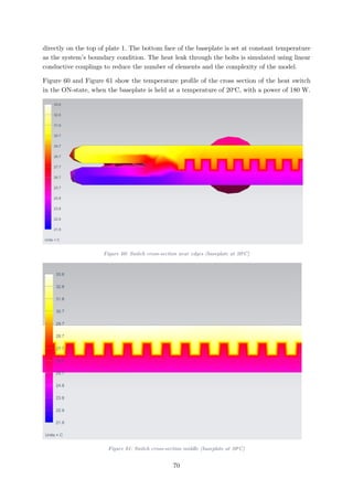
![candidate for the gas-gap heat switch, since it is the gas with the highest thermal conductivity.
Consequently, in this chapter, the simulations were run for both Helium and Hydrogen to
provide an indication of the improvement in performance. Figure 63 shows the overall ON-
conductance (including contact conductance) of the heat switch with respect to the effective
area. The effective area is defined as the flat surface in contact with the unit and the heat
sink. The figure shows that the ON-case heat transfer coefficient reaches a plateau around at
0.06 m2
, with a value of 232 W/m2
∙K for Helium and 241 W/m2
∙K for Hydrogen. This
represents an improvement of the overall ON-conductance by 3.9%. For the smaller sizes, the
heat transfer coefficient is higher since the in-plane heat spread is more efficient and heat can
be conducted more efficiently through the sidewalls.
Figure 63: ON-conductance scale analysis
In the OFF-case, an effective emissivity of 0.263 is applied for the radiative coupling from one
side of the switch to the other, an approximation explained in detail in section 5.5.1. The solid
mesh representing the gas is deactivated, assuming zero conduction through the gas. Figure
64 shows the overall heat transfer coefficient (including contact conductance) for the OFF-
case with respect to the effective area. Similarly to the ON-case, the heat transfer coefficient
is significantly higher at smaller sizes of the heat switch, since conduction through the sidewalls
dominates. With increasing size, the heat is conducted less efficiently in-plane through the thin
faces (0.7 mm) as the conductive thermal resistance increases. As a result, the radiation across
the gap starts dominating as the main heat transfer mode. From the graph, it can be seen that
the curve has not yet reached a convergence as good as in the ON-case. For a 30x30 cm2
switch, the OFF-case heat transfer coefficient is 9.28 W/m2
∙K, whereas for a 35x35 cm2
switch
it is 8.83 W/m2
∙K. This yields and overall ON/OFF ratio of 27.3 for Hydrogen and 26.3 for
Helium. Further simulations were impossible to be carried out because of computational
resources limitations. Tens of millions of elements are necessary for larger sizes of the heat
switch.
0
50
100
150
200
250
300
350
0 0.01 0.02 0.03 0.04 0.05 0.06 0.07 0.08 0.09 0.1
Heattransfercoefficient[W/m2∙K]
Area [m2]
h (He) h (H2)
72](https://image.slidesharecdn.com/ab16c9ba-74cc-44a4-aa76-d5a97c25dce8-160912051601/85/AE5810-Thesis-85-320.jpg)
![Figure 64: OFF-conductance scale analysis
For the ON and OFF-case, we have a good indication of the ideal performance of the heat
switch, by making a plausible assumption for the contact heat transfer coefficient that is based
on the experimental results of Chapter 8. According to the information provided for the units
of Sentinel-2, a heat switch of 0.1 m2
is required under the batteries. For this size, both the
ON and OFF heat transfer coefficient have reached significant convergence. In order to confirm
these models, further testing is necessary with parts manufactured with good tolerances and
in vacuum facilities that can accommodate such sizes. Though, it should be noted that the ON
and OFF heat transfer coefficients are still far from the requirement values of 500 and 5
W/m2
∙K respectively and therefore far from the ratio of 100. For the performance requirements,
please refer to Table 1 in section 3.3.1.
Figure 65 shows the area density of the heat switch with respect to the effective area. The
area density converges to a value of 8.16 kg/m2
, when the effective area is larger than 0.1 m2
.
This value violates the minimum requirement of 8.0 kg/m2
established in Table 1.
Figure 65: Heat switch area density
0
5
10
15
20
25
30
35
0 0.01 0.02 0.03 0.04 0.05 0.06 0.07 0.08 0.09 0.1 0.11 0.12 0.13
Heattransfercoefficient[W/m2∙K]
Area [m2]
0
2
4
6
8
10
12
0 0.01 0.02 0.03 0.04 0.05 0.06 0.07 0.08 0.09 0.1 0.11 0.12 0.13
Areadensity[kg/m2]
Area [m2]
73](https://image.slidesharecdn.com/ab16c9ba-74cc-44a4-aa76-d5a97c25dce8-160912051601/85/AE5810-Thesis-86-320.jpg)
![7.8 Test procedure
The test procedure for the third prototype is outlined with the following steps:
1. Set tank pressure regulator to 2 bar
2. Open all valves to purge the switch
3. Pump the gas (Helium) out
4. Perform bake-out at 80o
C
5. Pressurize gas to 1.7 bar (exceed the continuum regime limit) using the pressure
regulator
6. Set the baseplate temperature at -40o
C
7. Set the heater power at 180 W
8. Wait for system stabilization. For the stabilization criteria, see section 7.9
9. Increase baseplate temperatures by increments of 20o
C until +40o
C
10. Turn OFF the heater
11. Depressurize the switch using the rotary pump below molecular regime pressure limit
12. Repeat steps 6 to 9. Instead of 180 W, apply 15 W respectively
13. Switch Helium tank with Neon tank
14. Repeat steps 1 to 14
Ultimately, the performance of the switch should be dependent only on its temperature. More
specifically, in the ON-state, the switch conductance increases with increasing temperature
due to the increasing thermal conductivity of the gases. In the OFF-state, the switch
conductance increases with increasing temperature, since the radiative heat transfer inside the
gap increases. For the second prototype, the test procedure is identical with the only differences
being that the applied power in the ON-case is 40 W and in the OFF-case 5 W and that no
testing with Neon is necessary. It should be reminded that only Helium and Neon were
eventually considered for conducting the test because of the safety constraints at ESTEC that
prohibit the use of Hydrogen.
7.9 Test stabilization criteria
The stabilization criterion is critical when performing a thermal balance test, since it defines
whether the tested system has reached thermal equilibrium. The stabilization criterion can be
specified as a maximum rate of change of the temperature (𝑑𝑑𝑑𝑑/𝑑𝑑𝑑𝑑), as a specified temperature
difference 𝛥𝛥𝑇𝑇𝑡𝑡𝑡𝑡𝑡𝑡𝑡𝑡𝑡𝑡𝑡𝑡 from the steady-state or a combination of both. However, a temperature
difference requirement is problematic, since the true steady-state temperature is not accurately
known prior to testing, especially for powered test setups, and can only be approximated with
simulations [37].
A full finite element model takes several hours to solve for both the ON and OFF case because
of the large number of elements and the complicated couplings between them. For this reason,
a simplified thermal network was generated in ThermXL, using lumped masses. This network
is very useful in the correlation process between the simulation and experimental data as it
provides results that are comparable to the finite element model, within a few seconds.
Consequently, this network can be adjusted iteratively in order to provide an initial correlation
74](https://image.slidesharecdn.com/ab16c9ba-74cc-44a4-aa76-d5a97c25dce8-160912051601/85/AE5810-Thesis-87-320.jpg)
![Figure 67: Lumped mass test setup transient response at 20o
C (ON-case)
Figure 68: FEM test setup transient response at 20o
C (ON-case)
The lumped-mass model and the FEM for the OFF-case are very well correlated too. Using
second order exponential curve fitting for the two models, the individual time constant for the
top of the switch is 27.7 minutes and 30.8 minutes respectively.
15
20
25
30
35
40
0 200 400 600 800 1000 1200 1400 1600 1800 2000
Temperature[oC]
Time [sec]
Plate 1 top Top switch Bottom switch Plate 2 top Baseplate top
15
20
25
30
35
40
0 200 400 600 800 1000 1200 1400 1600 1800 2000
Temperature[oC]
Time [sec]
Plate 1 top Switch top Switch bottom
76](https://image.slidesharecdn.com/ab16c9ba-74cc-44a4-aa76-d5a97c25dce8-160912051601/85/AE5810-Thesis-89-320.jpg)
![Figure 69: Lumped mass test setup transient response at 20o
C (OFF-case)
Figure 70: FEM test setup transient response at 20o
C (OFF-case)
In preparation for the test, a preliminary stabilization criterion can be determined using the
concept of the “terminal time constant”. In this method, the thermal network is described by
a system of N simultaneous first-order differential equations that follow the energy balance
equation [38]:
𝑐𝑐𝑛𝑛
𝑑𝑑𝑑𝑑𝑛𝑛
𝑑𝑑𝑑𝑑
= 𝑝𝑝𝑛𝑛 − � 𝐺𝐺𝑛𝑛,𝑞𝑞�𝑇𝑇𝑛𝑛 − 𝑇𝑇𝑞𝑞� − � 𝐺𝐺𝑛𝑛,𝑏𝑏(𝑇𝑇𝑛𝑛 − 𝑇𝑇𝑏𝑏)
𝑁𝑁𝑏𝑏
𝑏𝑏=1
𝑁𝑁
𝑞𝑞=1
(𝑛𝑛 = 1,2, … , 𝑁𝑁) (7.9-1)
15
20
25
30
35
40
45
0 2000 4000 6000 8000 10000 12000
Temperature[oC]
Time [sec]
Plate 1 top Top switch Bottom switch Plate 2 top Baseplate top
15
20
25
30
35
40
45
0 2000 4000 6000 8000 10000 12000
Temperature[oC]
Time [sec]
Plate 1 top Top switch Bottom switch
77](https://image.slidesharecdn.com/ab16c9ba-74cc-44a4-aa76-d5a97c25dce8-160912051601/85/AE5810-Thesis-90-320.jpg)
![Where 𝑁𝑁 is the number of nodes, 𝑐𝑐𝑛𝑛 is the heat capacity of node 𝑛𝑛 and 𝑝𝑝𝑛𝑛 is the power
dissipation. 𝐺𝐺𝑛𝑛,𝑞𝑞 represents the internal conductances of the system (conductive, convective or
radiative) and 𝐺𝐺𝑛𝑛,𝑏𝑏 the external conductances, i.e. conductances to the boundaries. For this
equation to hold true, the radiative conductances need to be linearized according to equation
(5.1-1). This linearization is very accurate when relatively small temperature differences occur,
such as the ones expected in the case of the heat switch. Eventually, the equations are reduced
to [38]:
𝑇𝑇𝑛𝑛(𝑡𝑡) = 𝑣𝑣𝑛𝑛 + � 𝑏𝑏𝑘𝑘 𝑢𝑢𝑘𝑘,𝑛𝑛 𝑒𝑒 𝜆𝜆𝑘𝑘 𝑡𝑡
𝑁𝑁
𝑞𝑞=1
(7.9-2)
Where 𝜆𝜆𝑘𝑘 represents the eigenvalue. The eigenvalue is negative so that the nodes can converge
to a steady state temperature. The 𝑣𝑣𝑛𝑛 coefficient is determined from the boundary conditions.
The eigenvalue and 𝑢𝑢𝑘𝑘,𝑛𝑛 are determined by the characteristics of the network and 𝑏𝑏𝑘𝑘 from the
initial conditions of the network. Eventually, the terminal constant is defined as [38]:
𝜏𝜏∞ = −
1
𝜆𝜆 𝑚𝑚
(7.9-3)
Where 𝜆𝜆 𝑚𝑚 is the minimum absolute eigenvalue. The terminal time constant differs from the
individual time constant, as it represents the limit value of the time constant common to all
the diffusive nodes of the network.
For the second prototype, for the ON-case, 𝜆𝜆 𝑚𝑚 = |−0.0054294|, which corresponds to a
terminal constant of 184 seconds or 3.1 minutes. For the OFF-case, 𝜆𝜆 𝑚𝑚 = |−0.00060453|,
which corresponds to a terminal constant of 1,654 seconds or 27.6 minutes.
For the third prototype, for the ON-case, 𝜆𝜆 𝑚𝑚 = |−0.0025581|, which corresponds to a terminal
constant of 6.5 minutes. For the OFF-case, 𝜆𝜆 𝑚𝑚 = |−0.00038792|, which corresponds to a
terminal constant of 43.0 minutes.
The allowable rate of rate of change of the temperature is dictated by the accuracy of the
thermocouples and the time constant. As explained later in section 9.4, thermocouples have
usually an overall accuracy of about ±0.2o
C. Thus, a rate of change less than 𝛥𝛥𝑇𝑇𝑗𝑗 = 1 𝐾𝐾 over
a period 𝛥𝛥𝛥𝛥 = 𝜏𝜏∞ is a typically set as a criterion for every node j. More relaxed duration criteria
can be used when the previous requirement is impossible to be satisfied. Though, to preserve
minimum significance of a thermal balance test, a temperature change of 1 K over a minimum
𝛥𝛥𝛥𝛥 =
𝜏𝜏∞
3
is the limit. The maximum deviation with respect to the ideal stabilization
temperature can be determined as:
𝜀𝜀𝑗𝑗,𝑚𝑚𝑚𝑚𝑚𝑚 =
�𝛥𝛥𝑇𝑇𝑗𝑗�
𝑒𝑒
𝛥𝛥𝛥𝛥
𝜏𝜏∞ − 1
(7.9-4)
For 𝛥𝛥𝛥𝛥 equal to 𝜏𝜏∞,
𝜏𝜏∞
2
and
𝜏𝜏∞
3
, the maximum deviation is 0.58 K, 1.54 K and 2.52 K
respectively.
78](https://image.slidesharecdn.com/ab16c9ba-74cc-44a4-aa76-d5a97c25dce8-160912051601/85/AE5810-Thesis-91-320.jpg)
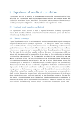
![Figure 71: Sigraflex contact heat transfer coefficient for second prototype
8.1.2 Third prototype
Figure 72 and Figure 73 show the contact heat transfer coefficients with respect to temperature
for the third prototype for the OFF and ON-case respectively. Because in the third prototype,
the setup is experiencing more severe deviations in the contact heat transfer coefficient with
temperature variations, a temperature dependent heat transfer coefficient has been
implemented in the thermal model.
Figure 72: Sigraflex contact heat transfer coefficient for third prototype (OFF-case)
y = -1.7334x + 603.25
y = 2.477x + 769.42
0
100
200
300
400
500
600
700
800
900
1000
-50 -40 -30 -20 -10 0 10 20 30 40 50
Contactheattransfercoefficient[W/m2·K]
Baseplate [oC]
Top switch
Bottom switch
y = 0.0686x2 - 2.3733x + 653.21
y = 0.035x2 + 8.2903x + 767.16
0
200
400
600
800
1000
1200
1400
-50 -40 -30 -20 -10 0 10 20 30 40 50
Contactheattransfercoefficient[W/m2·K]
Baseplate [oC]
Top switch
Bottom switch
81](https://image.slidesharecdn.com/ab16c9ba-74cc-44a4-aa76-d5a97c25dce8-160912051601/85/AE5810-Thesis-94-320.jpg)
![Figure 73: Sigraflex contact heat transfer coefficient for third prototype (ON-case)
8.2 Real time constant calculations
The real-time constant methodology is used in order to validate that the system has reached
steady-state. In this methodology, the experimental time rate of change of the temperature
𝑑𝑑𝑑𝑑/𝑑𝑑𝑑𝑑 is monitored with respect to time. More precisely, a backwards difference of 3 minutes
is used for each time step, which is normalized per minute and then curve-fitted using an
exponential function. The inverse of the curve fit exponent yields the time constant. It should
be noted that as the system approaches steady-state, an increased scattering is caused due to
the increased relative effect of thermocouple measurement instabilities. Consequently, such
data points are not included in the curve fitting [37]. Eventually, the stabilization criterion is
taken as:
𝑑𝑑𝑑𝑑
𝑑𝑑𝑑𝑑
�
𝑡𝑡𝑡𝑡𝑡𝑡𝑡𝑡𝑡𝑡𝑡𝑡
=
𝛥𝛥𝑇𝑇𝑡𝑡𝑡𝑡𝑡𝑡𝑡𝑡𝑡𝑡𝑡𝑡
𝜏𝜏
.
𝛥𝛥𝑇𝑇𝑡𝑡𝑡𝑡𝑡𝑡𝑡𝑡𝑡𝑡𝑡𝑡 is selected to be 0.2o
C which is defined by the accuracy of the thermocouples.
8.2.1 Second prototype
8.2.1.1 ON-state
For the ON-case, the terminal time constant from section 7.9, which represents a system
averaged time constant, was found to be 3.07 minutes. The FEM yields a theoretical time
constant of 3.58 minutes for the top of the switch. The real time constant of the top of the
switch was experimentally determined to be 4.48 minutes, a 25.1% difference. This difference
is the direct result of the performance of the heat switch in its ON-state, when it is pressurized
with Helium. The higher the ON-conductance of the heat switch the smaller the time constant.
As it can be seen from Figure 82 in section 8.2.1.1, the actual performance of the heat switch
at +20o
C, when applying a power of 40 W is at 74.2% of the theoretical value and consequently
longer dwell time is required for temperature stabilization. Figure 75 provides a comparison
y = 0.0142x2 - 0.5654x + 673.67
y = 0.0163x2 + 1.8742x + 593.89
0
100
200
300
400
500
600
700
800
-60 -40 -20 0 20 40 60
Contactheattransfercoefficient[W/m2∙K]
Baseplate [oC]
Top switch
Bottom switch
82](https://image.slidesharecdn.com/ab16c9ba-74cc-44a4-aa76-d5a97c25dce8-160912051601/85/AE5810-Thesis-95-320.jpg)
![between the experimental and the FEM results for the ON-case transient response at a nominal
baseplate temperature of 20o
C. It should be noted that due to instability problems controlling
the baseplate temperature, there is an inconsistent offset between the experimental and the
theoretical baseplate temperature.
Figure 74: Second prototype real time constant - ON-state (20o
C)
Figure 75: Second prototype ON-case transient response (20o
C)
y = 6.9952e-0.223x
y = 5.309e-0.279x
0.001
0.01
0.1
1
10
0 5 10 15 20 25 30 35
dT/dt[oC/min]
Time [min]
Experimental Theoretical
15
20
25
30
35
40
45
0 5 10 15 20 25 30 35
Temperature[oC]
Time [min]
Plate 1 top Switch top Switch bottom Baseplate
Plate 1 - FEM Switch top - FEM Switch bottom - FEM
83](https://image.slidesharecdn.com/ab16c9ba-74cc-44a4-aa76-d5a97c25dce8-160912051601/85/AE5810-Thesis-96-320.jpg)
![8.2.1.2 OFF-state
For the OFF-case, the terminal time constant from section 7.9 was found to be 27.56 minutes
For the OFF-case, the FEM yields a theoretical time constant of 30.6 minutes for the top of
the switch. The same real time constant was experimentally determined to be 21.1 minutes, a
-31.0% difference. This difference is the direct result of the performance of the heat switch in
its OFF-state. The higher the OFF-conductance of the heat switch the smaller the time
constant. As it can be seen from Figure 91 in section 8.2.1.2, the heat transfer coefficient of
the heat switch at +20o
C, when applying a power of 5 W is 26.6% higher than the theoretical
value. However, it should be noted that the baseplate exhibited significant instability during
the test for the evaluation of the time constant. This can be seen from Figure 77, where the
baseplate, the switch and plate 1 exhibit periodic fluctuations with a period of 66 minutes.
Based on the temperature profile, the top and the bottom of the switch are out of phase by
about 15 minutes. Throughout a mission lifetime, the baseplate of a unit experiences periodic
temperature variations. Consequently, the phase difference provides an indication of the
responsiveness of the switch.
Figure 76: Second prototype real time constant - OFF-state (20o
C)
y = 0.7163e-0.0474x
y = 0.7037e-0.0327x
0.01
0.1
1
0 20 40 60 80 100 120 140
dT/dt[oC/min]
Time [min]
Experimental Theoretical
84](https://image.slidesharecdn.com/ab16c9ba-74cc-44a4-aa76-d5a97c25dce8-160912051601/85/AE5810-Thesis-97-320.jpg)
![Figure 77: Second prototype OFF-case transient response (20o
C)
8.2.2 Third prototype
8.2.2.1 ON-state
For the ON-case, the terminal time constant from section 7.9 was found to be 6.52 minutes.
The FEM yields a theoretical time constant of 6.45 minutes for the top of the switch. The real
time constant of the top of the switch was experimentally determined to be 12.44 minutes, a
92.8% increase. This difference is the direct result of the performance of the heat switch in its
ON-state, when pressurized with Helium. As it can be seen from Figure 90 in section 8.3.1.2,
the actual performance of the heat switch at +20o
C, when applying a power of 50 W is at only
14.8% of the theoretical value and consequently longer dwell time is required for temperature
stabilization. Because of this significant deviation in performance, a heating power of 50 W is
used instead of 180 W as mentioned in section 7.8. Figure 78 provides a comparison between
the experimental and the FEM results for the ON-case transient response at a nominal
baseplate temperature of 20o
C. As can be seen from Figure 79, the baseplate temperature could
not be maintained stable during the heating process of the system and increased from 16.5o
C
to 23o
C, when the rest of the system reached stability, indicated by the plateau of the
temperatures.
15
20
25
30
35
40
45
0 50 100 150 200 250 300
Temperature[oC]
Time [min]
Plate 1 Switch top Switch bottom Baseplate
Plate 1 - FEM Switch top - FEM Switch bottom - FEM
85](https://image.slidesharecdn.com/ab16c9ba-74cc-44a4-aa76-d5a97c25dce8-160912051601/85/AE5810-Thesis-98-320.jpg)
![Figure 78: Third prototype real time constant - ON-state (20o
C)
Figure 79: Third prototype ON-case transient response (20o
C)
8.2.2.2 OFF-state
For the OFF-case, the terminal time constant from section 7.9 was found to be 43.0 minutes
For the OFF-case, the FEM yields a theoretical time constant of 44.9 minutes for the top of
the switch. The real time constant of the top of the heat switch was experimentally determined
to be 23.9 minutes, a -46.8% difference. Similarly to the second prototype, the difference is the
direct result of the performance of the heat switch in its OFF-state. As it can be seen from
Figure 94 in section 8.3.2.2, the heat transfer coefficient of the heat switch at +20o
C, when
applying a power of 15 W is 89.8% higher than the theoretical value, which entails a significant
y = 1.5819e-0.0804x
y = 0.9512e-0.155x
0.01
0.1
1
10
0 5 10 15 20 25 30 35
dT/dt[oC/min]
Time [min]
Experimental Theoretical
15
20
25
30
35
40
0 20 40 60 80 100 120 140 160 180
Temperature[oC]
Time [min]
Plate 1 Switch top Switch bottom Baseplate
Plate 1 - FEM Switch top - FEM Switch bottom - FEM
86](https://image.slidesharecdn.com/ab16c9ba-74cc-44a4-aa76-d5a97c25dce8-160912051601/85/AE5810-Thesis-99-320.jpg)
![decrease in the time constant. It should be noted that in this case, the baseplate exhibited a
much better stability compared to Figure 77, providing better accuracy in the estimation of
the real time constant.
Figure 80: Third prototype real time constant - OFF-state (20o
C)
Figure 81: Third prototype OFF-case transient response (20o
C)
y = 0.6734e-0.0419x
y = 0.66755e-0.02229x
0.01
0.1
1
0 10 20 30 40 50 60 70 80 90
dT/dt[oC/min]
Time [min]
15
20
25
30
35
40
45
50
55
0 20 40 60 80 100 120 140 160 180 200
Temperature[oC]
Time [min]
Plate 1 Switch top Switch bottom Baseplate
Plate 1 - FEM Switch top - FEM Switch bottom
87](https://image.slidesharecdn.com/ab16c9ba-74cc-44a4-aa76-d5a97c25dce8-160912051601/85/AE5810-Thesis-100-320.jpg)
![8.3 ON/OFF conductances
8.3.1 ON-conductance
8.3.1.1 Second prototype
Figure 82 shows the experimental and theoretical values of the heat transfer coefficient across
the heat switch in its ON-state with respect to the baseplate temperature, when a power of 40
W is applied on Plate 1. All measurements were performed at a controlled pressure of 1.7 bar,
thus exceeding the theoretical continuum regime pressure limit of ≈1 bar for Helium. The
experimental measurements show a degraded performance when compared to the theoretical
values of the FEM. Additionally, the curve of the experimental data has a steeper slope than
the theoretical curve. The gas thermal conductivity values were obtained from the NIST
Chemistry WebBook, which states “The uncertainty in thermal conductivity is 5%, except at
low temperatures where it increases to 10%”. Such uncertainty cannot fully justify this
deviation. The differences can be attributed to impurities in the operating gas and the
geometry of the heat switch. The impurities in the operating gas can stem from a) the gas
tank, b) mixing of helium with ambient air due to tubing leakage, c) trapped air in the switch.
The switch is 3D-printed and consequently cavities with trapped air can be created during
manufacturing. To minimize the effect of trapped air in the switch, a thermal bake-out was
performed at a temperature of +80o
C prior to testing. Furthermore, as shown in section 6.3,
there is a significant deviation of the actual gap distance from the nominal. The gap distance
is critical for the performance of the switch, since a larger gap filled with a gas that has low
thermal conductivity leads to a significantly degraded performance. Unfortunately, the actual
gap distance after mounting of the test setup cannot be measured and consequently cannot be
taken into account for the theoretical results. Moreover, because of the inaccessibility between
the aluminium plates and the switch, only one thermocouple per surface is used and
consequently heat spread is not taken into account in this measurement. This can explain the
deviation from the theoretical values.
Figure 82: Second prototype ON-state heat transfer coefficient (P = 40 W)
y = 2.06x + 445.66
y = 0.4704x + 646.62
0
100
200
300
400
500
600
700
-60 -40 -20 0 20 40 60
Heattransfercoefficient[W/m2·K]
Baseplate [oC]
Experimental Theoretical
88](https://image.slidesharecdn.com/ab16c9ba-74cc-44a4-aa76-d5a97c25dce8-160912051601/85/AE5810-Thesis-101-320.jpg)
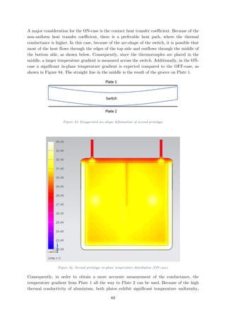
![with temperature variations of only 0.2o
C. Therefore, the location of the thermocouples is not
critical and there is an essential reduction in the uncertainty.
Figure 85: Second prototype ON-state overall heat transfer coefficient (Plate 1 to Plate 2)
As can be seen from Figure 85, the FEM is much better correlated with the experimental
values when compared to Figure 82. The pink curve in Figure 85 indicates the overall heat
transfer coefficient when a temperature-dependent thermal conductivity for Ti-6Al-4V is used.
This dependency is more critical in the OFF-case. For more information, please see section
8.3.2. The experimental data still exhibits a higher sensitivity on temperature. This sensitivity
is most likely the result of the uncertainty in the contact heat transfer coefficient. Additionally,
because of the thermal expansion and contraction with varying temperatures, the gap size
changes, a factor that has not been taken into account in the theoretical model. Moreover, the
applied torque on the fasteners changes with changes in temperature, thus affecting the contact
heat transfer coefficient. Eventually, the model exhibits maximum deviation of +19.9% at -
40o
C and -9.6% at +40o
C. At 20o
C, the deviation is only 3.9%.
8.3.1.2 Third prototype
Initially, it was intended to apply a heat load of 180 W for the ON-case of the third prototype
as mentioned in section 7.8. However, because of the low ON-conductance, a lower power was
applied in order to not generate an excessive gradient that could harm the equipment. Figure
86 shows the experimental and theoretical values of the heat transfer coefficient across the
heat switch in its ON-state (Helium) with respect to the baseplate temperature, when a power
of 50 W is applied on Plate 1. All measurements were performed at a controlled pressure of
1.7 bar, thus exceeding the theoretical continuum regime pressure limit of ≈1 bar for Helium.
Similarly to the second prototype, the overall heat transfer coefficient from Plate 1 to Plate 2
is provided in Figure 87.
y = 0.9826x + 243.1703
y = 0.0647x + 240.1273
y = 0.1349x + 249.88
0
50
100
150
200
250
300
350
-60 -40 -20 0 20 40 60
Heattransfercoefficient[W/m2·K]
Baseplate [oC]
Experimental Theoretical adjusted k
90](https://image.slidesharecdn.com/ab16c9ba-74cc-44a4-aa76-d5a97c25dce8-160912051601/85/AE5810-Thesis-103-320.jpg)
![Figure 86: Third prototype ON-state heat transfer coefficient (P = 50 W)
Figure 87: Third prototype ON-state overall heat transfer coefficient (Plate 1 to Plate 2)
The experimental measurements show a significantly degraded performance when compared
to the theoretical values of the FEM. This degradation stems from the severe deviation of the
manufactured third prototype from the CAD model as explained in section 6.3.2. Due to its
larger area compared to the second prototype, the third prototype cannot be flattened easily,
even when applying a high bolt torque. This is because the bolt pattern is perimetric and the
pressure in the middle is not greatly affected. Consequently, the gaps in the middle of the
switch cannot be reduced significantly and reach a value closer to the nominal as happened
with the second prototype. Unfortunately, the actual gap distance after mounting of the test
setup cannot be measured directly. However, the effective gap distance can be estimated by
repeating the test under similar conditions with another gas. More specifically, another round
of testing was repeated for the third prototype using Neon as the active gas. At a baseplate
temperature of 20o
C, the total thermal resistance from plate 1 to plate 2 was measured at
0.36925 o
C/W and 0.30500 o
C/W for Neon and Helium respectively. For simplification of the
y = 0.0007x2 + 0.2783x + 101.15
y = -0.0056x2 + 1.6068x + 646.14
0
100
200
300
400
500
600
700
800
-60 -40 -20 0 20 40 60
Heattransfercoefficient[W/m2∙K]
Baseplate [oC]
Experimental Theoretical
y = 0.0007x2 + 0.1842x + 76.601
y = 0.0013x2 + 0.3474x + 194.86
0
50
100
150
200
250
-60 -40 -20 0 20 40 60
Heattransfercoefficient[W/m2∙K]
Baseplate [oC]
Experimental Theoretical
91](https://image.slidesharecdn.com/ab16c9ba-74cc-44a4-aa76-d5a97c25dce8-160912051601/85/AE5810-Thesis-104-320.jpg)
![calculations, all the leak conductive and radiative conductances from Figure 66 can be
neglected, since the leak power is estimated at only 2% according to section 9.2. Gcond is the
total conductance represented in Figure 21. The two experiments showed insignificant
differences in the contact conductances through the Sigraflex and consequently we can assume
they are equal. In this case, the thermal networks consists of multiple thermal resistances in
series that are identical, except for the gas resistance. The difference between the two
experimental total resistances provides the difference between the resistances of the two gases.
𝛥𝛥𝑅𝑅𝑡𝑡𝑡𝑡𝑡𝑡𝑡𝑡𝑡𝑡 = 𝑅𝑅𝑁𝑁𝑁𝑁 − 𝑅𝑅𝐻𝐻𝐻𝐻 =
𝐿𝐿𝑒𝑒𝑒𝑒𝑒𝑒
𝐴𝐴
�
1
𝑘𝑘𝑁𝑁𝑁𝑁
−
1
𝑘𝑘𝐻𝐻𝐻𝐻
� (8.3-1)
With 𝑘𝑘𝑁𝑁𝑁𝑁 = 0.0476 𝑊𝑊/𝑚𝑚 ∙ 𝐾𝐾 and 𝑘𝑘𝐻𝐻𝐻𝐻 = 0.1535 𝑊𝑊/𝑚𝑚 ∙ 𝐾𝐾 at 20o
C, the ratio of the area to the
effective gap is
𝐴𝐴
𝐿𝐿𝑒𝑒𝑒𝑒𝑒𝑒
= 226. Using the nominal dimensions, the ratio is:
�
𝐴𝐴
𝐿𝐿
�
𝑛𝑛𝑛𝑛𝑛𝑛
=
0.0930
0.2 ∙ 10−3
= 465 (8.3-2)
Comparing the two results and using the nominal area of 0.0930 m2
, we see that the effective
gap is 2.06 times the nominal, which translates into 0.412 mm. Section 8.4.2 provides an
estimation of the effective gap size of the third prototype by measuring the pressure of the
transition into the continuum regime for Helium. The two methods are in very good agreement
and result in an effective gap that is twice as large as the nominal one.
Figure 88 and Figure 89 provide the experimental and theoretical values of the heat transfer
coefficient of switch and the overall heat transfer coefficient respectively, for the ON-case using
Neon. A heating power of 25 W is applied. A smaller power is applied, when compared to
Helium in order to avoid overheating due to the smaller thermal conductivity of Neon, which
entails a worse ON-conductance.
Figure 88: Switch heat transfer coefficient (Neon)
y = 0.1679x + 81.502
y = 0.5885x + 265.01
0
50
100
150
200
250
300
350
-60 -40 -20 0 20 40 60
Heattransfercoefficient[W/m2∙K]
Baseplate [oC]
Experimental Theoretical
92](https://image.slidesharecdn.com/ab16c9ba-74cc-44a4-aa76-d5a97c25dce8-160912051601/85/AE5810-Thesis-105-320.jpg)
![Figure 89: Overall heat transfer coefficient (Neon)
8.3.2 OFF-conductance
8.3.2.1 Second prototype
Figure 91 shows the experimental and theoretical values of the heat transfer coefficient across
the heat switch in its OFF-state with respect to the baseplate temperature, when a power of
5 W is applied on Plate 1. The initial predictions indicated by the green curve exhibited a
deviation of -13.0% to -20.2% from the experimental values. An important parameter that
adds some uncertainty in the simulations is the thermal conductivity of the material. Initially,
in the simulations, the thermal conductivity of Ti-6Al-4V was considered to be independent
of the temperature, with a constant value of 6.7 W/m∙K. Figure 90, obtained from the Military
Handbook for “Metallic Materials and Elements for Aerospace Vehicle Structures” (MIL-
HDBK-5H), shows the dependence of the thermal conductivity of some titanium alloys with
respect to temperature. In the temperature range of -40o
C to +60o
C, the thermal conductivity
of the alloy changes from 6.4 to 7.5 W/m∙K, a 17.2% increase, which is significant for the
OFF-case. The pink curve on Figure 91 shows the heat transfer coefficient of the heat switch
with the adjusted thermal conductivity. This led to a better correlation between the
experimental and theoretical data, with a deviation from -11.8% at -40o
C to -16.2% at +40o
C
baseplate temperature.
y = 0.1336x + 65.306
y = 0.2686x + 138.03
0
20
40
60
80
100
120
140
160
-60 -40 -20 0 20 40 60
Heattransfercoefficient[W/m2∙K]
Baseplate [oC]
Experimental Theoretical
93](https://image.slidesharecdn.com/ab16c9ba-74cc-44a4-aa76-d5a97c25dce8-160912051601/85/AE5810-Thesis-106-320.jpg)
![Figure 90: Effect of temperature on titanium alloys thermal conductivity
Another important consideration is the uncertainty on the emissivity of the internal surfaces
of the heat switch. As mentioned in section 6.1, the emissivity measurement was conducted
on the smoother external surface. Increasing roughness leads to an increase in the emissivity
and consequently a larger heat transfer coefficient. An increase of the emissivity from 0.57 to
0.62, combined with the adjustment for the thermal conductivity closed the gap between the
experimental and theoretical values (-10.3% to -12.6%). However, this emissivity value is
simply an assumption and cannot be measured exactly.
Figure 91: Second prototype OFF-state heat transfer coefficient (P = 5 W)
2.0
3.0
4.0
5.0
6.0
7.0
8.0
9.0
-220 -170 -120 -70 -20 30 80 130
Thermalconductivity[W/m∙K]
Temperature [oC]
Ti-6Al-4V Ti-5Al-2.5Sn Ti-6Al-6V-2Sn
y = 0.151x + 30.243
y = 0.0855x + 24.564
y = 0.1061x + 25.603
y = 0.1178x + 26.655
0
5
10
15
20
25
30
35
40
-50 -40 -30 -20 -10 0 10 20 30 40 50
Heattransfercoefficient[W/m2·K]
Baseplate [oC]
Experimental Theoretical Adjusted k Adjusted k and ε
94](https://image.slidesharecdn.com/ab16c9ba-74cc-44a4-aa76-d5a97c25dce8-160912051601/85/AE5810-Thesis-107-320.jpg)
![The remaining deviations can be attributed to other factors that cannot be controlled or
quantitatively be taken into account, such as the deviation of the manufactured heat switch
from the CAD model. The internal features of the heat switch have an impact on the
performance. This is true especially when the applied bolt torque is taken into account. The
applied torque deforms the heat switch, reducing the gaps between the fins, especially since
the support pillars have cracked. A reduction in the gap distance is translated into an increase
in the view factors between the fin surfaces, which leads to an increased radiative conductance.
It is possible that some of the fins are so deformed that they come in contact, providing an
additional parasitic heat path.
In order to minimize the internal pressure, the rotary pump kept running continuously
throughout testing of the OFF-case to provide a vacuum of less than 10-4
mbar. Such low
pressure is measured by an additional pressure sensor placed at the outlet of the pressure line.
Since it is impossible to place a pressure sensor inside the heat switch, there is an uncertainty
about the pressure in the cavity of the switch. It is possible that some gas molecules remain
trapped inside the miniscule channels of the switch and with increasing temperature these
molecules conduct more heat.
Similarly to the ON-case, to the overall gradient from Plate 1 to Plate 2 can be found. In this
case the deviation of the theoretical from the experimental value is from -11.8% to -16.2%.
Figure 92: Second prototype OFF-state overall heat transfer coefficient (Plate 1 to Plate 2)
In the OFF-case, the temperature of the two faces is more uniform and only small in-plane
gradients occur. This can be proved by comparing Figure 93 with Figure 84. Therefore, the
temperature measurements are more representative in the OFF-case and are independent of
the thermocouple location.
y = 0.1245x + 27.9114
y = 0.0786x + 23.0998
y = 0.0925x + 23.766
y = 0.1022x + 24.66
0
5
10
15
20
25
30
35
-50 -40 -30 -20 -10 0 10 20 30 40 50
Heattransfercoefficient[W/m2·K]
Baseplate [oC]
Experimental Theoretical Adjusted k Adjusted k and ε
95](https://image.slidesharecdn.com/ab16c9ba-74cc-44a4-aa76-d5a97c25dce8-160912051601/85/AE5810-Thesis-108-320.jpg)
![Figure 94: Third prototype OFF-state heat transfer coefficient (P = 15 W)
This significant difference can be explained by the deviation of the manufactured third
prototype from the original CAD model, such as the increased thickness, which leads to a
smaller thermal resistance. The theoretical mass of the third prototype is 335.3 g. However,
the measurements showed a mass of 354.6 g, a 5.8% increase, which could partially explain
the deviation in the OFF-conductance. It is also possible that at some locations the fins are
touching the other side of the switch similarly to Figure 30. Additionally, the uncertainty
about the pressure inside the cavity of the switch remains. Consequently, it is possible that
trapped gas molecules conduct heat across the channels.
Figure 95 shows the overall gradient from Plate 1 to Plate 2. This graph removes any
uncertainties stemming from the thermocouples placement, since the overall experimental heat
transfer coefficient remains almost double the theoretical one and it proves that the third
prototype does not operate in its ideal performance.
Figure 95: Third prototype OFF-state overall heat transfer coefficient (Plate 1 to Plate 2)
y = 0.00057x2 + 0.07092x + 25.03499
y = 0.04709x + 13.11619
0
5
10
15
20
25
30
35
-60 -40 -20 0 20 40 60
Heattransfercoefficient[W/m2∙K]
Baseplate [oC]
Experimental Theoretical
y = 0.00052x2 + 0.06785x + 23.38977
y = 0.00016x2 + 0.04412x + 12.55221
0
5
10
15
20
25
30
-60 -40 -20 0 20 40 60
Heattransfercoefficient[W/m2∙K]
Baseplate [oC]
Experimental Theoretical
97](https://image.slidesharecdn.com/ab16c9ba-74cc-44a4-aa76-d5a97c25dce8-160912051601/85/AE5810-Thesis-110-320.jpg)
![8.4 Conductance dependence on pressure
As mentioned in section 5.3, the pressure inside the switch is very critical for its performance,
as it dictates the thermal conductivity of the gas. Even though the test setup passed the initial
inspections for the leak rate, both prototypes showed a significant pressure drop throughout
the experiment. The leak test was conducted at room temperature, while the test temperature
range was between -40o
C and +40o
C for the baseplate. Due to the mismatch of the CTE
between stainless steel and Ti-6Al-4V, the materials contract and expand differently. Thus,
when the baseplate temperature is reduced to its minimum value of -40o
C, there is some
loosening of the tubing connection, which in turn leads to a leak. Typically, this loosening is
permanent, even if the temperature is increased, as the nuts need to be retorqued. It should
be noted that controlling the pressure below 1 bar is very difficult. Consequently, this leak
provided an opportunity to measure the performance of the heat switch with respect to
pressure in a controlled manner.
8.4.1 Second prototype
The pressure drop for the second prototype is shown in Figure 96. The scatter after 1500
minutes is the result of the resolution of the data acquisition system and the sensor. However,
the exponential trendline appears to fit accurately the obtained data with a constant exponent
coefficient.
Figure 96: Second prototype pressure drop
Problems with the PID controller of the vacuum facility resulted in instabilities of the
baseplate temperature, which exhibited periodic fluctuations of up to 5o
C peak-to-valley with
a sharp change rate similar to Figure 77. These instabilities produced spikes in the estimation
of the heat transfer coefficient. To smooth the spikes, the moving average method was used.
y = 1,801.017271e-0.003055x
1
10
100
1000
10000
0 500 1000 1500 2000 2500
Pressure[mbar]
Time [min]
98](https://image.slidesharecdn.com/ab16c9ba-74cc-44a4-aa76-d5a97c25dce8-160912051601/85/AE5810-Thesis-111-320.jpg)
![The heat transfer coefficient of the heat switch with respect to pressure is shown in Figure 97.
The lower limit of the measurements is dictated by the resolution of the data acquisition
system and the lower limit of the pressure sensor (1.33 mbar).
In Figure 97, the heat transfer coefficient has an S-shape as expected, similar to Figure 22 and
Figure 23. Figure 98 is a magnification of the 200 to 1800 mbar range that shows the shift
from the transition to the continuum regime. The plateau value is around 450 W/m2
∙K at a
pressure just above 1 bar. This value is in good agreement with the estimated value of 958
mbar from section 5.3.4. At the lower limit, the heat transfer coefficient keeps decreasing with
decreasing pressure, which confirms that the gas remains in the transition regime and has not
yet shifted to the molecular regime. Unfortunately, because of the baseplate instabilities, it is
not possible to distinguish the expected transition jump as explained in section 5.3.
Figure 97: Heat transfer coefficient against pressure (second prototype)
0
50
100
150
200
250
300
350
400
450
500
1 10 100 1000 10000
Heattransfercoefficient[W/m2∙K]
Pressure [mbar]
99](https://image.slidesharecdn.com/ab16c9ba-74cc-44a4-aa76-d5a97c25dce8-160912051601/85/AE5810-Thesis-112-320.jpg)
![Figure 98: Transition to continuum regime heat transfer coefficient (second prototype)
8.4.2 Third prototype
The third prototype eventually exhibited a leak, despite passing the initial leakage rate
inspection. Figure 99 shows the Helium pressure drop over time. Due to scattering because of
the sensitivity of the sensor close to its lower limit, points below a pressure of 40 mbar are
removed from the graph to allow for a better exponential curve fitting.
Figure 99: Third prototype pressure drop
Figure 100 shows the performance of the heat switch with respect to pressure, when the
baseplate is maintained at an average temperature of 17.86o
C. Problems with the baseplate
instability remained during testing of the third prototype as well. However, the baseplate
exhibited improved behavior with a maximum deviation of 2o
C and a standard deviation of
0
50
100
150
200
250
300
350
400
450
500
0 200 400 600 800 1000 1200 1400 1600 1800 2000
Heattransfercoefficient[W/m2∙K]
Pressure [mbar]
y = 1,686.20722e-0.00152x
1
10
100
1000
10000
0 500 1000 1500 2000 2500 3000
Pressure[mbar]
Time [min]
100](https://image.slidesharecdn.com/ab16c9ba-74cc-44a4-aa76-d5a97c25dce8-160912051601/85/AE5810-Thesis-113-320.jpg)
![0.338o
C. Because of the temperature fluctuations of the baseplate, the moving average
approach has been used. Figure 100 shows that the third prototype reaches a plateau for the
heat transfer coefficient at around 500 mbar. This plateau corresponds to the transition to the
continuum regime. The reduced value of this transition pressure compared to the value of 1000
mbar for the second prototype confirms that even after torqueing the bolts with 0.85 N·m, the
effective gap between the two sides of the switch is about double according to equations (5.3-1)
and (5.3-2). This result is in very good agreement with the result obtained using a different
method in section 8.3.1.2. Consequently, because of this excessive gap, the performance of the
third prototype in its ON-state is severely degraded compared to its theoretical value as is
shown in section 8.3.1.2. At the lower limit, of the graph, the heat transfer coefficient keeps
decreasing with decreasing pressure, and therefore, the molecular regime limit has not yet been
reached.
Figure 100: Heat transfer coefficient against pressure (third prototype)
8.5 ON/OFF ratio
The ON/OFF ratio is the most important indicator of the performance of a heat switch. The
function of the ON/OFF ratio with respect to temperature can be found be taking the ratio
of the two experimental trendlines for the overall heat transfer coefficient.
Thus, for the second prototype:
𝑅𝑅𝑂𝑂𝑂𝑂/𝑂𝑂𝑂𝑂𝑂𝑂 =
0.9826 ∙ 𝑇𝑇 + 243.1703
0.1245 ∙ 𝑇𝑇 + 27.9114
For the third prototype:
𝑅𝑅𝑂𝑂𝑂𝑂/𝑂𝑂𝑂𝑂𝑂𝑂 =
0.0013 ∙ 𝑇𝑇2
+ 0.3474 ∙ 𝑇𝑇 + 194.86
0.00052 ∙ 𝑇𝑇2 + 0.0679 ∙ 𝑇𝑇 + 23.39
0
20
40
60
80
100
120
1 10 100 1000 10000
Heattransfercoefficient[W/m2·K]
Pressure [mbar]
h switch h overall
101](https://image.slidesharecdn.com/ab16c9ba-74cc-44a4-aa76-d5a97c25dce8-160912051601/85/AE5810-Thesis-114-320.jpg)
![Figure 101: Third prototype ON/OFF ratio
Figure 102: Third prototype ON/OFF ratio
8.6 Summary
Detailed Finite Element Models and reduced Thermal Mathematical Models have been created
for the prediction of the behavior of the developed gas-gap heat switch. The conducted
experiments have shown that these models are within 11.8% to 16.2% accurate for the OFF-
case and -19.9% to 9.6% for the ON-case for the second prototype. Such differences are deemed
satisfactory, especially given the deviation of the manufactured prototype from the CAD model
used in the Finite Element Analysis and the uncertainties in the thermal contact conductances.
For the third prototype, the FEM is off by a factor of 2 for the OFF-case and a factor of 6 for
0
5
10
15
20
25
30
35
-50 -40 -30 -20 -10 0 10 20 30 40 50
RON/OFF
Temperature [oC]
Switch - Experimental Switch - Theoretical
Overall - Experimental Overall Theoretical
0
10
20
30
40
50
60
-50 -40 -30 -20 -10 0 10 20 30 40 50
RON/OFF
Baseplate [oC]
Switch - Experimental Switch - Theoretical
Overall - Experimental Overall - Theoretical
102](https://image.slidesharecdn.com/ab16c9ba-74cc-44a4-aa76-d5a97c25dce8-160912051601/85/AE5810-Thesis-115-320.jpg)

![9 Uncertainty analysis
“Uncertainty is a quantification of the doubt about the measurement results” [39]. For proper
interpretation of the results, a measurement uncertainty analysis was performed. This is
because, even for the most careful measurements there is always a margin of uncertainty that
can be attributed to the measurement process, the measuring instrument or even uncontrolled
factors, such as environmental ones.
In the case of the heat switch experiment, the measurement in question is the heat transfer
coefficient in the ON and OFF state. The governing equation for the measurement is thus:
ℎ𝑂𝑂𝑂𝑂,𝑂𝑂𝑂𝑂𝑂𝑂 =
𝑃𝑃ℎ𝑒𝑒𝑒𝑒𝑒𝑒𝑒𝑒𝑒𝑒 − 𝑃𝑃𝑙𝑙 𝑙𝑙𝑙𝑙𝑙𝑙
𝐴𝐴(𝑇𝑇ℎ − 𝑇𝑇𝑐𝑐)
(8.6-1)
𝑃𝑃ℎ𝑒𝑒𝑒𝑒𝑒𝑒𝑒𝑒𝑒𝑒 is the power generated by the heater, 𝑃𝑃𝑙𝑙 𝑙𝑙𝑙𝑙𝑙𝑙 is the power that leaks through the system,
𝐴𝐴 is the cross-section area, 𝑇𝑇ℎ is the temperature measured on the hot side and 𝑇𝑇𝑐𝑐 on the cold
side. Because the temperatures and the heating power are measured by separate instruments,
they are independent of each other. In this case, the relative uncertainty of the heat
conductance can be expressed using the root sum of squares:
𝑑𝑑ℎ𝑂𝑂𝑂𝑂,𝑂𝑂𝑂𝑂𝑂𝑂
ℎ𝑂𝑂𝑂𝑂,𝑂𝑂𝑂𝑂𝑂𝑂
= 𝑘𝑘 ∙ ��
𝑑𝑑𝑑𝑑ℎ𝑒𝑒𝑒𝑒𝑒𝑒𝑒𝑒𝑟𝑟 + 𝑑𝑑𝑑𝑑𝑙𝑙 𝑙𝑙𝑙𝑙𝑙𝑙
𝑃𝑃ℎ𝑒𝑒𝑒𝑒𝑒𝑒𝑒𝑒𝑒𝑒 − 𝑃𝑃𝑙𝑙 𝑙𝑙𝑙𝑙𝑙𝑙
�
2
+ �
𝑑𝑑𝑑𝑑𝑙𝑙 𝑙𝑙𝑙𝑙𝑙𝑙
𝑃𝑃𝑙𝑙 𝑙𝑙𝑙𝑙𝑙𝑙
�
2
+ �
𝑑𝑑𝑑𝑑
𝐴𝐴
�
2
+ �
𝑑𝑑𝑑𝑑ℎ + 𝑑𝑑𝑑𝑑𝑐𝑐
(𝑇𝑇ℎ − 𝑇𝑇𝑐𝑐)
�
2
(8.6-2)
The numerator of each component indicates their respective standard uncertainty and the
denominator their nominal value.
This combined uncertainty was multiplied by a coverage factor 𝑘𝑘 = 2, for a confidence level
of 95%, assuming the combined standard uncertainty follows a normal distribution.
9.1 Heating power uncertainty
The heating power supplied to the test setup is determined by measuring the voltage across
the power supply terminals using the multimeter of the data acquisition unit. In this case, the
power can be calculated using 𝑃𝑃 =
𝑉𝑉2
𝑅𝑅
. However, because long wires are used to connect the
heater to the electrical feedthrough of the chamber and from the feedthrough to the power
supply, wire resistances are introduced. Typically, a four-point measurement can be
implemented for more accurate results, where two separate pairs of electrodes measure the
current and the voltage across the heater resistance. The measurement of the electrical
resistances of the heater and of the heater with the wires showed an increase of the resistance
by less than 0.1%. Consequently, these losses can be neglected. However, these measurements
were conducted at room temperature. The electrical resistance of the wires changes with
temperature. Consequently, for more accurate measurements the current through the circuit
was measured using the ammeter of the power supply. The heating power can then be
established simply using 𝑃𝑃 = 𝑉𝑉 ∙ 𝐼𝐼. The accuracy of the measurement of the DC voltage is
104](https://image.slidesharecdn.com/ab16c9ba-74cc-44a4-aa76-d5a97c25dce8-160912051601/85/AE5810-Thesis-117-320.jpg)
![9.3 Area uncertainty
The external dimensions of the heat switch were measured with a Vernier caliper with an
uncertainty of 0.01 mm. Consequently, for a nominal contact area of 210 mm x 210 mm, the
uncertainty is less than 0.007%. This value is insignificant relative to the other uncertainties
and can therefore be neglected in the combined uncertainty budget.
9.4 Thermocouples uncertainty
For the test, Type K thermocouples were used. The thermocouples were calibrated in
accordance with the requirements of ISO/IEC 17025 “General requirements for the competence
of testing and calibration laboratories” and following the instructions of ESA’s TEC-MTV-
MSL/D001 document for “Calibration of Thermocouple Sensors”. Four calibration points were
used; -195.8o
C (boiling point of LN2), -100o
C, 0o
C and +75o
C. Figure 103 shows the curve of
the temperature difference between each thermocouple and the calibration points. As expected,
the deviation from the calibration point is minimized at room temperature. Third order
polynomial curve fitting was used to establish the calibration equations that were implemented
in the Data Acquisition Controller to obtain accurate temperature measurements.
Figure 103: T/C temperature difference with calibration points (second prototype)
The combined uncertainty budget of the thermocouples includes uncertainties of the working
standard calibration and uncertainties of the measurements during calibration. Eventually, the
combined uncertainty budget with a coverage factor of 2 is less than 0.16o
C within the test
temperature range of -40o
C to +40o
C. The uncertainty of the thermocouples with respect to
temperature is plotted in Figure 104.
-0.5
0
0.5
1
1.5
2
2.5
3
3.5
4
-250 -200 -150 -100 -50 0 50 100
ΔT=TT/C-Tcal[oC]
Tcal [oC]
Te1 Te2 Te3 Te4 Te5 Te6 Te7 Te8
Ti1 Ti2 Ti3 Ti4 Ti5 Ti8 TH1 TH2
106](https://image.slidesharecdn.com/ab16c9ba-74cc-44a4-aa76-d5a97c25dce8-160912051601/85/AE5810-Thesis-119-320.jpg)
![Figure 104: Combined T/C uncertainty budget
9.5 Sample uncertainty calculations
Below a sample calculation for the uncertainty of the overall ON and OFF heat transfer
coefficient of the second prototype at a baseplate temperature of 20o
C is given. The overall
heat transfer coefficient refers to the gradient from Plate 1 to Plate 2.
𝑑𝑑ℎ𝑂𝑂𝑂𝑂
ℎ𝑂𝑂𝑂𝑂
= 2 ∙ ��
0.486 + 0.088
39.935 − 0.439
�
2
+ �
0.16 + 0.16
(39.53 − 24.10)
�
2
= 5.1%
𝑑𝑑ℎ𝑂𝑂𝑂𝑂𝑂𝑂
ℎ𝑂𝑂𝑂𝑂𝑂𝑂
= 2 ∙ ��
0.126 + 0.116
5.012 − 0.581
�
2
+ �
0.16 + 0.16
(34.75 − 18.15)
�
2
= 11.6%
9.6 Summary
An uncertainty analysis for the obtained values of the heat transfer coefficient was performed.
The uncertainty parameters are considered to be independent of each other and the combined
uncertainty can be obtained using the root sum of squares. The estimated uncertainties are
provided with a confidence level of 95%. The uncertainty for the OFF-case is more than double
the uncertainty of the ON-case, which is attributed mainly to the higher heat leak relative to
the supplied power.
0
0.05
0.1
0.15
0.2
0.25
0.3
-200 -150 -100 -50 0 50 100
CombinedUncertainty[oC]
Measured Temperature [oC]
107](https://image.slidesharecdn.com/ab16c9ba-74cc-44a4-aa76-d5a97c25dce8-160912051601/85/AE5810-Thesis-120-320.jpg)
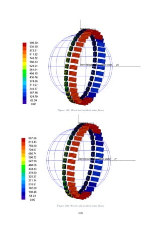
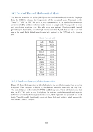
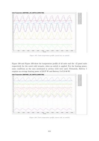
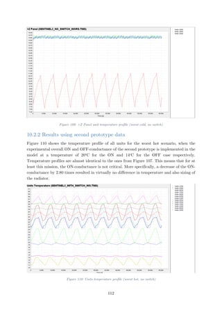
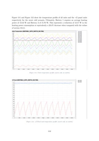
![Apart from the minimum feature size, another important aspect of manufacturing is the
flatness and surface roughness of the heat switch. The manufactured prototypes have so far
exhibited significant flatness problems due to buckling that stems from residual thermal
stresses generated during production. In order to further reduce these residual stresses a
combination of the lattice structure from Figure 34 with an increase in the thickness of the
top and bottom faces of the heat switch can be used. The increased thickness of the two faces
will facilitate the heat spreading and the heat sinking to the build-plate of the structure.
Furthermore, it provides additional torsional stiffness that will prevent the buckling effect.
Following the annealing process, the extra material will be shaved off using face milling or
grinding as shown in Figure 115 to reduce the thickness to its nominal value of 0.7 mm.
Grinding is preferable since the dimensions of the heat switch are similar to that of a sheet of
metal. Consequently, milling can generate excessive shear stresses, it will last longer and will
provide a worse surface roughness.
Figure 115: Milling versus grinding process [40]
This material shaving will provide an ideal flatness and surface roughness that are critical for
the proper mounting of the switch, especially when taking into account the contact thermal
conductance. Additionally, the surface roughness of the tubes is also critical, as it is affects
the leakage at the interface with the tube fittings. Increased roughness creates voids through
which the gas is easier to escape. Consequently, the thickness of the tubes can be locally
increased and then reduced to the nominal diameter using face milling to provide an improved
surface finish.
A cost analysis is necessary to determine whether the cost of the excessive material is an
inhibiting factor. With a simple market research, the cost of Ti-6Al-4V powder is about 250-
500 €/kg. Adding a conservative thickness of 5 mm per side corresponds to a surface mass
density of 44.3 kg/m2
. Thus, the excessive material cost per area taking the maximum price
of 500 €/kg is 22,150 €/m2
, which corresponds to 11% of the total cost per area charged for
the latest prototype. Through this basic cost analysis, it is confirmed that this is a viable
option. A more elaborate cost analysis would be beneficial to determine also the marginal cost,
which represents the cost added by producing one extra unit of the product.
117](https://image.slidesharecdn.com/ab16c9ba-74cc-44a4-aa76-d5a97c25dce8-160912051601/85/AE5810-Thesis-130-320.jpg)
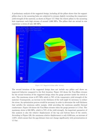
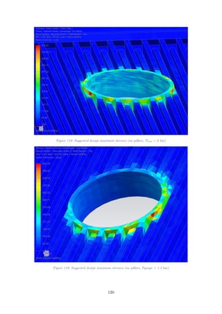
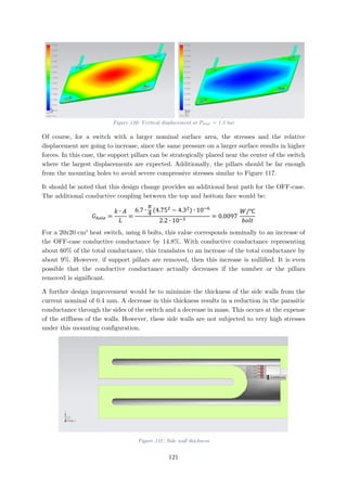
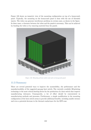
![Another important parameter to be taken into account is the leakage rate of the switch. A
proper sealing must be applied on the tubes of the switch in order to minimize the gas losses.
As a first solution, materials with matching CTE should be used to minimize the relative
displacement of the components with changes in temperature. Furthermore, interference
problems between the tubes and the panels shall be taken into account. A potential solution
would be the bending of the tubes at a 90o
angle, facing away from the panel.
Once an efficient and accurate manufacturing process has been established, for better
understanding of its behavior, the heat switch shall be subjected to thermal fatigue tests. This
is to determine the thermal cycles it can undergo before failure in order to determine its
survivability during a real-life mission. Accelerated thermal cycling with sharp temperature
fluctuations could be used. Creep refers to the deformation of materials at elevated
temperatures when they are exposed to static mechanical stresses [41]. Because the heat switch
is not expected to reach very high temperatures (T<0.4Tmelting [K]), creep should not be an
issue, unless the switch is used on hot space structures.
125](https://image.slidesharecdn.com/ab16c9ba-74cc-44a4-aa76-d5a97c25dce8-160912051601/85/AE5810-Thesis-138-320.jpg)
![Appendix A Sentinel-2 units
Table 25: Units power dissipation and temperature range
Unit
Dissipation Min [W] Dissipation Max [W]
Operational
Temperature Range
[o
C]
Sun Eclipse Sun Eclipse Min Max
COMS 69 27.6 70 28.3 -10 +50
Batteries 0 10 0 22.5 +9 +35
PCDU 83 52 95 60 -20 +55
SBT 33.6+6.7 33.6+6.7 33.6+6.7 33.6+6.7 -15 +88
WDE 19.4 19.4 30.4 30.4 -20 +50
MMFU 39 30 50 37 -20 +45
ICU 89 14.6 99 16.3 -20 +50
GPS 9.6 9.6 12.4 12.4 -20 +50
OBC 23 23 24.2 24.2 -20 +50
RIU 41.5 41.5 47.3 47.3 -20 +50
Table 26: Acronyms, dimensions and thermal capacitance of Sentinel-2 units
Unit Acronym
Base Dimension [mm] Thermal
Capacitance
[J/K]
Length Width
COMS Communications 1000 950 10000
Batteries - 360 280 25066
PDCU
Power Conditioning and
Distribution Unit
510 330 27400
SBT S-Band Transponder 180 170 2461
WDE Wheel Drive Electronics 270 240 7689
MMFU
Mass Memory and
Formatting Unit
330 300 9068
ICU Instrument Control Unit 360 360 24600
GPS Global Positioning System 310 220 2765
OBC On-board Computer 200 220 9000
RIU Remote Interface Unit 460 210 14160
126](https://image.slidesharecdn.com/ab16c9ba-74cc-44a4-aa76-d5a97c25dce8-160912051601/85/AE5810-Thesis-139-320.jpg)
![Appendix B Orbital heating fluxes
Figure 123: Incident Albedo flux in Worst Hot
Figure 124: Incident Albedo flux in Worst Cold
0
50
100
150
200
250
300
350
400
450
500
0 1000 2000 3000 4000 5000 6000 7000
AlbedoFlux[W/m2]
Orbit Time [s]
Albedo = 0.4
-X
-Y
-Z
+Z
+Y
+X
0
50
100
150
200
250
0 1000 2000 3000 4000 5000 6000 7000
AlbedoFlux[W/m2]
Orbit Time [s]
Albedo = 0.2
-X
-Y
-Z
+Z
+Y
+X
127](https://image.slidesharecdn.com/ab16c9ba-74cc-44a4-aa76-d5a97c25dce8-160912051601/85/AE5810-Thesis-140-320.jpg)
![Figure 125: Incident Solar flux in Worst Hot
Figure 126: Incident Solar flux in Worst Cold
0
200
400
600
800
1000
1200
1400
0 1000 2000 3000 4000 5000 6000 7000
SolarFlux[W/m2]
Orbit Time [s]
-X
-Y
-Z
+Z
+Y
+X
0
200
400
600
800
1000
1200
1400
0 1000 2000 3000 4000 5000 6000 7000
SolarFlux[W/m2]
Orbit Time [s]
-X
-Y
-Z
+Z
+Y
+X
128](https://image.slidesharecdn.com/ab16c9ba-74cc-44a4-aa76-d5a97c25dce8-160912051601/85/AE5810-Thesis-141-320.jpg)
![Appendix C Material transport properties
Table 27: Lennard-Jones constants and molecular weights of selected species [15]
129](https://image.slidesharecdn.com/ab16c9ba-74cc-44a4-aa76-d5a97c25dce8-160912051601/85/AE5810-Thesis-142-320.jpg)
![Table 28: Collision integrals for diffusivity, viscosity, and thermal conductivity based on the Lennard-Jones
potential [15]
130](https://image.slidesharecdn.com/ab16c9ba-74cc-44a4-aa76-d5a97c25dce8-160912051601/85/AE5810-Thesis-143-320.jpg)
![Appendix D Gas thermal properties8
Figure 127: Gases thermal conductivity with respect to temperature
The uncertainty in the density is 0.2% for Hydrogen, 1.0% for Helium and 0.1% for Neon.
Figure 128: Gases density with respect to temperature
The uncertainty in the thermal conductivity is 10% for Hydrogen, 1.0% for Helium and 5%
for Neon.
The properties were obtained at the theoretical continuum boundary of 700 mbar for
Hydrogen, 1000 mbar for Helium and 140 mbar for Neon.
8
All properties are obtained from NIST Chemistry WebBook
0
0.05
0.1
0.15
0.2
0.25
0.3
-100 -80 -60 -40 -20 0 20 40 60 80 100
Density[kg/m3]
Temperature [oC]
Hydrogen Helium Neon
0
0.05
0.1
0.15
0.2
0.25
-100 -80 -60 -40 -20 0 20 40 60 80 100
Thermalconductivity[W/m·K]
Temperature [oC]
Hydrogen Helium Neon
131](https://image.slidesharecdn.com/ab16c9ba-74cc-44a4-aa76-d5a97c25dce8-160912051601/85/AE5810-Thesis-144-320.jpg)
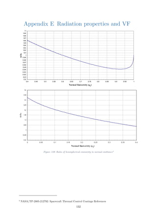
![Figure 131: Second prototype fin profile
Table 29: Second prototype fin view factors
View Factor Area [m2
]
F1→2 0.8384 2.5∙10-5
F1→8 0.1616 2.5∙10-5
F3→4 0.8658 1.4∙10-4
F3→8 0.0412 1.4∙10-4
F5→6 0.1348 3.25∙10-4
F5→4 0.1757 2∙10-5
F7→4 0.0412 2∙10-5
F7→6 0.1009 2∙10-5
134](https://image.slidesharecdn.com/ab16c9ba-74cc-44a4-aa76-d5a97c25dce8-160912051601/85/AE5810-Thesis-147-320.jpg)
![Figure 132: Third prototype fin profile
Table 30: Third prototype fin view factors
View Factor Area [m2
]
F1→2 0.8384 5∙10-5
F1→8 0.1616 5∙10-5
F3→4 0.6180 8∙10-5
F3→8 0.1280 8∙10-5
F5→6 0.1348 6.5∙10-5
F5→4 0.1258 4∙10-5
F7→4 0.1280 4∙10-5
F7→6 0.1009 4∙10-5
� 𝐴𝐴𝑖𝑖 𝐹𝐹𝑖𝑖𝑖𝑖
7
𝑖𝑖=1
= 𝐴𝐴1 𝐹𝐹12 + 2𝐴𝐴1 𝐹𝐹18 + 2𝐴𝐴3 𝐹𝐹34 + 2𝐴𝐴3 𝐹𝐹38 + 2𝐴𝐴5 𝐹𝐹54 + 2𝐴𝐴5 𝐹𝐹56 + 2𝐴𝐴7 𝐹𝐹74 + 2𝐴𝐴7 𝐹𝐹76
135](https://image.slidesharecdn.com/ab16c9ba-74cc-44a4-aa76-d5a97c25dce8-160912051601/85/AE5810-Thesis-148-320.jpg)
![Appendix F Material properties
Table 31: Ti-6Al-4V chemical composition11
Element Percentage
Ti 89.734%
Al 6%
V 4%
Others 0.266%
Table 32: Inconel 718® chemical composition12
Element Percentage
Ni 53%
Cr 20%
Fe 17%
Nb 5%
Mo 3%
Ti 1%
Others 1%
Table 33: Material thermal properties
Material ρ [kg/m3
] k [W/m·K] Cp [J/kg·K] α [1/K]
Aluminium 606113
2,711 167 896 22.38∙10-6
A2-70 SS14
8,000 16.2 500 17.3∙10-6
Ti-6Al-4V15
4,430 6.7 526.3 8.6∙10-6
Inconel 718 8,190 11.4 435 13∙10-6
Table 34: Material structural properties
Material ρ [kg/m3
] E [GPa]
Poisson ratio
v
UTS [MPa]
YTS [MPa]
Ti-6Al-4V 4,430 121.0 0.342 845 805
Inconel 718 8,190 200.0 0.294 1375 1100
Aluminium
6061-T6
2,711 69.0 0.330 276 242
11
From MatWeb: Titanium Ti-6Al-4V (Grade 5), Annealed
12
From MatWeb: Special Metals INCONEL® Alloy 718
13
Values obtained at 20o
C from NX 9.0 material library
14
From MatWeb: 304 Stainless Steel (Austenitic)
15
From NX 9.0 material library
136](https://image.slidesharecdn.com/ab16c9ba-74cc-44a4-aa76-d5a97c25dce8-160912051601/85/AE5810-Thesis-149-320.jpg)
![A2-70 SS 8,000 190.0 0.300 700 450
PEEK 1,350 4.4 0.38 - -
Note that the Shear Modulus for isotropic materials is calculated as [41]:
𝐺𝐺 =
𝐸𝐸
2(1 + 𝑣𝑣)
(12.2-1)
Figure 133: Hydrogen permeability versus temperature [42]
137](https://image.slidesharecdn.com/ab16c9ba-74cc-44a4-aa76-d5a97c25dce8-160912051601/85/AE5810-Thesis-150-320.jpg)
![Appendix G Structural analysis results
Table 35: Classical rule-of-thumb safety factors [30]
Safety Factor Criteria
FSmaterial = 1.1 Material properties known from a handbook or are manufacturer’s values
FSstress = 1.3
Nature of the load is defined in an average manner, with overloads of
20-50% and the stress analysis may result in error <50%
FSgeometry = 1.1 Manufacturing tolerances are not closely held
FSfailure analysis = 1.0
Failure analysis is derived for the state of stress, as for uniaxial or
multiaxial static stresses or fully reversed uniaxial fatigue stresses
FSreliability = 1.2 For a reliability of 95%
Maximum bolt preload
Figure 134: Bolted connections contact pressure
138](https://image.slidesharecdn.com/ab16c9ba-74cc-44a4-aa76-d5a97c25dce8-160912051601/85/AE5810-Thesis-151-320.jpg)
![Figure 135: Test setup exaggerated displacement
Overpressurization
Figure 136: Switch exaggerated displacement [2.3 bar]
139](https://image.slidesharecdn.com/ab16c9ba-74cc-44a4-aa76-d5a97c25dce8-160912051601/85/AE5810-Thesis-152-320.jpg)


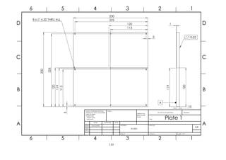
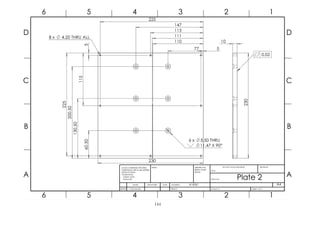
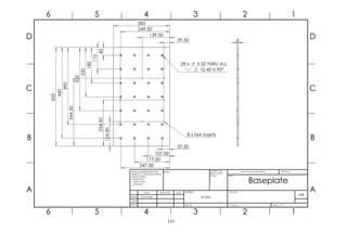
![References
[1] W. J. Larson and J. R. Wertz, Space Mission Analysis and Design, Microcosm Press and
Kluwer Academic Publishers, 2005.
[2] I. Catarino, G. Bonfait and L. Duband, "Neon gas-gap heat switch," Cryogenics, vol. 48,
no. 1-2, pp. 17-25, 2008.
[3] M. Krielaart, C. Vermeer and S. Vanapalli, "Compact flat-panel gas-gap heat switch
operating at 295 K," Review of Scientific Instruments, no. 86, 2015.
[4] J. C. Mankins, "Technology Readiness Levels," Office of Space Access and Technology -
NASA, 1995.
[5] European Cooperation for Space Standardization, ECSS-S-ST-00-01C - ECSS system -
Glossary of terms, Noordwijk, the Netherlands: ESA Requirements and Standards
Division, 2012.
[6] Y. A. Cengel and A. J. Ghajar, Heat and Mass Transfer, McGraw-Hill, 2011.
[7] J. R. Howell, R. Siegel and P. M. Menguc, Thermal Radiation Heat Transfer, New York:
McGraw-Hill, 2010.
[8] European Space Agency, "View Factors," European Space Agency, Noordwijk, the
Netherlands, 1989.
[9] J. Fatemi and M. H. J. Lemmen, "Effective Thermal/Mechanical Properties of
Honeycomb Core Panels for Hot Structure Applications," Journal of Spacecraft and
Rockets, vol. 46, no. 3, pp. 514-525, 2009.
[10] B. Gebhart, Heat Transfer, McGraw-Hill, 1961.
[11] C. Y. Han and J.-M. Choi, "Thermal Analysis of Spacecraft Propulsion System and its
Validation," KSME International Journal, vol. 18, no. 5, pp. 847-856, 2004.
[12] R. D. Karaman, Satellite Thermal Control for Systems Engineers, AIAA, 1998.
[13] D. G. Gilmore, Spacecraft Thermal Control Handbook, The Aerospace Press, 2002.
[14] J. J. Lissauer and I. de Pater, Fundamental Planetary Science: Physics, Chemistry and
Habitability, Cambridge University Press, 2013.
[15] J. H. Lienhard IV and J. H. Lienhard V, A heat transfer textbook, Cambridge, MA:
Phlogiston Press, 2003.
146](https://image.slidesharecdn.com/ab16c9ba-74cc-44a4-aa76-d5a97c25dce8-160912051601/85/AE5810-Thesis-159-320.jpg)
![[16] E. Anglada and I. Garmendia, "Correlation of thermal mathematical models for thermal
control of space vehicles by means of genetic algorithms," Acta Astronautica, vol. 108,
pp. 1-17, 2015.
[17] E. Tal-Gutelmacher and D. Eliezer, "Hydrogen-Assisted Degradation of Titanium Based
Alloys," Materials Transactions, vol. 45, no. 5, pp. 1594-1600, 2004.
[18] B. S. Yilbas, A. Coban, R. Kahraman and M. M. Khaled, "Hydrogen Embrittlement of
Ti-6Al-4V Alloy with Surface Modification by TiN Coating," International Journal
Hydrogen Energy, vol. 23, no. 6, pp. 483-489, 1998.
[19] M. Ando, K. Shinozaki, A. Okamoto, H. Sugita and T. Nohara, "Development of
Mechanical Heat Switch of Future Space Missions," in 44th International Conference on
Environmental Systems, Tucson, AZ, 2014.
[20] D. Mishkinis, J. Corrochano and A. Torres, "Development of Miniature Heat Switch-
Temperature Controller based on variable conductance LHP," in Second International
Conference "Heat Pipes for Space Applications", Moscow, 2014.
[21] M. Pauken, E. Sunada, K. Novak, C. Philips, G. Birur and K. Lankford, "Development
Testing of a Paraffin-Actuated Heat Switch for Mars Rover Applications," in
International Conference On Environmental Systems, San Antonio, TX, 2002.
[22] European Space Agency, "Sentinel-2: The operational Copernicus optical high resolution
land mission," ESA, Noordwijk, the Netherlands, 2013.
[23] E. E. Anderson and R. Viskanta, "Effective conductivity for conduction-radiation by
Taylor series expansion," Heat Mass Transfer International Journal, vol. 14, pp. 1220-
1224, 1971.
[24] M. Kaviany, Heat Transfer Physics, Cambridge University Press, 2008.
[25] B. R. Munson, D. F. Young, T. H. Okiishi and W. W. Huebsch, Fundamentals of Fluid
Mechanics, John Wiley & Sons, 2009.
[26] R. C. Reid, J. M. Prausnitz and B. E. Poling, The Properties of Gases and Liquids, New
York: McGraw-Hill, 1987.
[27] J. R. Thomas and D. P. Hasselmann, "Effect of Interfacial Separation on Composite
Thermal Conductivity," in 28th International Thermal Conductivity Conference and the
16th International Thermal Expansion Symposium, New Brunswick, Canada, 2005.
[28] G. Springer, "Heat transfer in rarefied gases," in Advances in Heat Transfer, Volume 7,
New York, Academic Press, 1971, pp. 163-218.
147](https://image.slidesharecdn.com/ab16c9ba-74cc-44a4-aa76-d5a97c25dce8-160912051601/85/AE5810-Thesis-160-320.jpg)
![[29] S. Song and M. M. Yovanovich, "Correlation of Thermal Accommodation Coefficient for
'Engineering' Surfaces," in Twenty-fourth National Heat Transfer Conference and
Exhibition, Pittsburgh, PA, 1987.
[30] F. P. Beer, R. E. Johnston Jr., J. T. DeWolf and D. F. Mazurek, Mechanics of Materials,
McGraw-Hill, 2012.
[31] C. Tien, "A correlation for thermal contact conductance of nominally-flat surfaces in a
vacuum," in Thermal Conductivity, Proceedings of the Seventh Conference, 1968.
[32] V. W. Antonetti, T. D. Whittle and R. E. Simons, "An approximate thermal contact
conductance correlation," Journal of Electronic Packaging, vol. 115, pp. 131-134, 1993.
[33] M. G. Cooper, B. B. Mikic and M. M. Yovanovich, "Thermal contact conductance,"
International Journal of Heat Mass Transfer, vol. 12, pp. 279-300, 1968.
[34] G. Meyer and D. Strelow, "Simple Diagrams Ain in Analysing Forces in Bolted Joints,"
Assembly Engineering, pp. 28-33, 1972.
[35] S. D. Rossides, "Behaviour of a Simple Tension Joint with Fasteners Tightened into
Yield," British Aerospace Report, 1981.
[36] D. G. Ullman, The Mechanical Design Process, New York: McGraw-Hill, 2010.
[37] S. L. Rickman and E. K. Ungar, "A physics-based temperature stabilization criterion for
thermal testing," in Aerospace Testing Conference, Manhattan Beach, CA, 2009.
[38] E. Colizzi, "Thermal Balance Testing: A Rigorous Theoretical Approach to Stabilisation
Criteria Based on Operative Re-Definition of Thermal Time Constant," in 42nd
International Conference on Environmental Systems, San Diego, CA, 2012.
[39] S. Bell, A Beginner's Guide to Uncertainty of Measurement, Teddington, Middlesex, UK:
National Physical Laboratory, 1999.
[40] J. Black and R. A. Kohser, De Garmo's Materials & Processes in Manufacturing, John
Wiley & Sons, 2008.
[41] W. D. Callister and D. G. Rethwisch, Material Science and Engineering, John Wiley &
Sons, 2011.
[42] McDonnel Douglas Astronautics Company, "Hydrogen in Titanium Alloys," McDonnel
Douglas Corporation, St Louis, 1981.
[43] Y. A. Cengel and M. A. Boles, Thermodynamics - An Engineering Approach, McGraw-
Hill, 2011.
[44] J.-R. Tsai, "Overview of Satellite Thermal Analytical Model," Journal of Spacecraft and
Rockets, vol. 41, no. 1, pp. 120-125, 2004.
148](https://image.slidesharecdn.com/ab16c9ba-74cc-44a4-aa76-d5a97c25dce8-160912051601/85/AE5810-Thesis-161-320.jpg)


![[IJET-V2I2P12] Authors:Ashok Kumar](https://cdn.slidesharecdn.com/ss_thumbnails/ijet-v2i2p12-160427185244-thumbnail.jpg?width=640&height=640&fit=bounds)


