Download to read offline


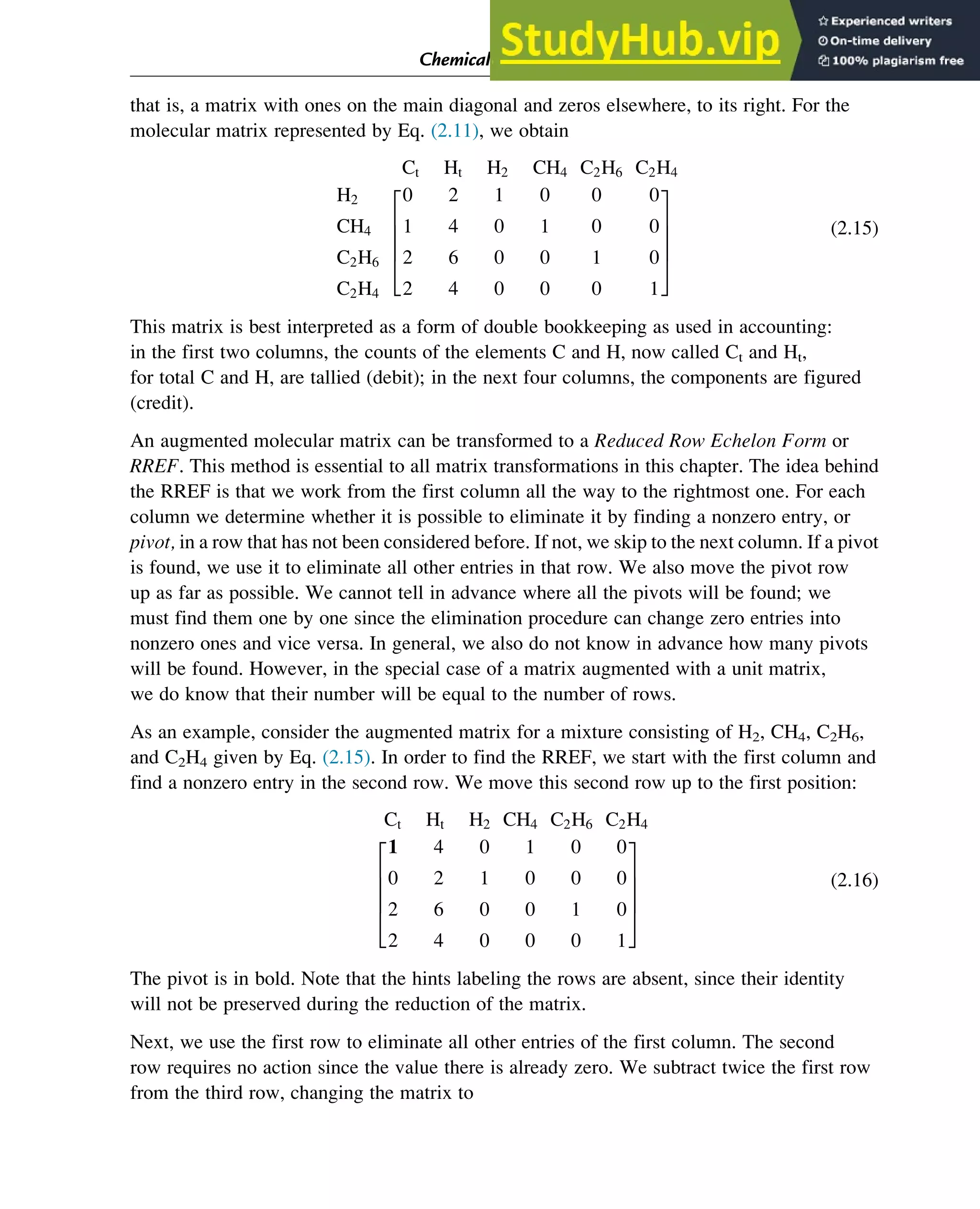
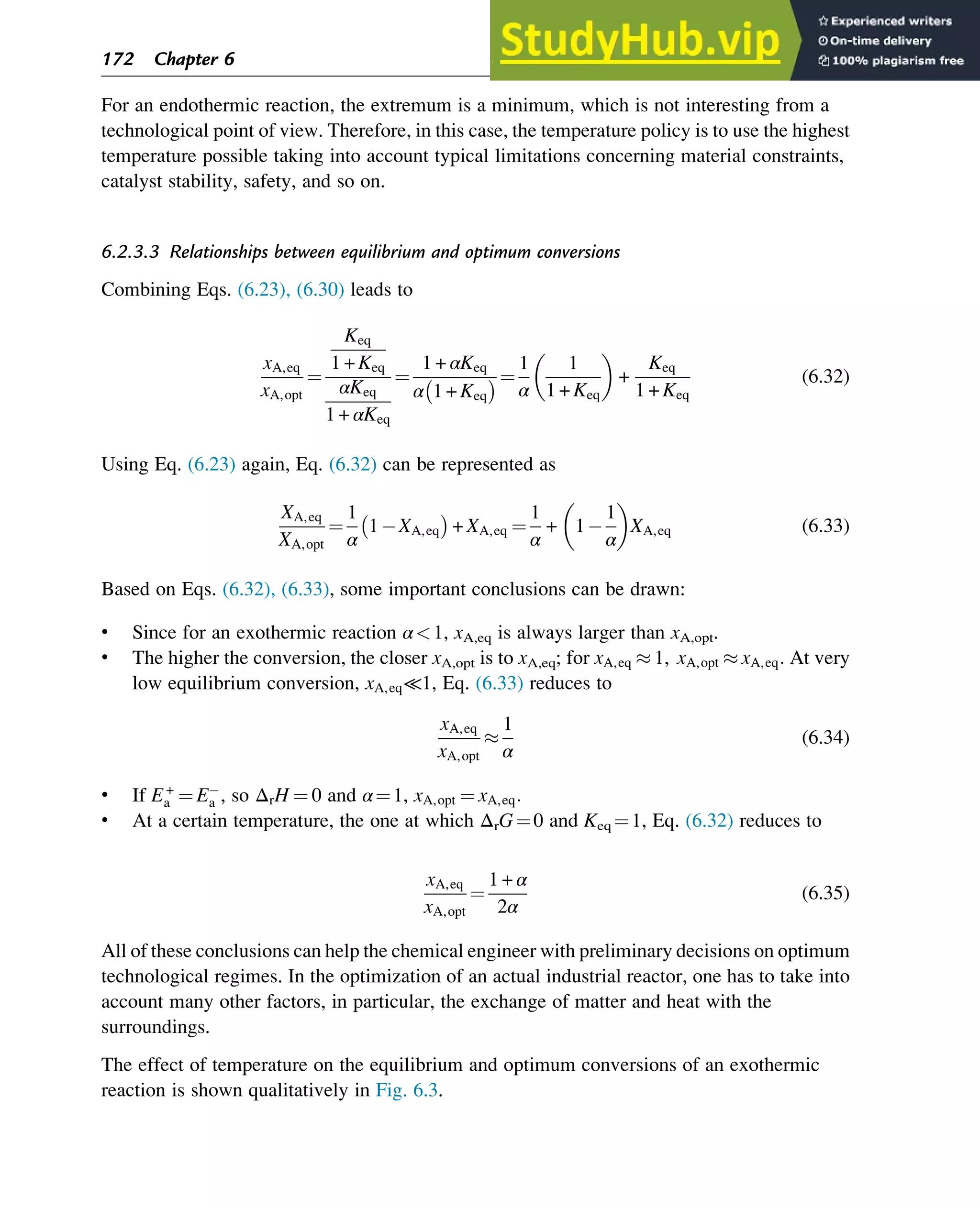
![# The number of rows m is the number of lists in the list
m ¼ len(a)
# The number of columns n is obtained from the first list; we assume but do not check
# that all lists in a have this same length
n ¼ len(a[1])
# Initially, no rows have been completed in the sense of having a pivot
rowsdone ¼ 0
# And no columns have been done either; but we traverse the n columns to work on them
# in this for loop
for columnsdone in range(n):
# Ignoring the rows that were done, we look for a nonzero entry in column i
i ¼ rowsdone
while i m and a[i][columnsdone] ¼¼ 0:
i ¼ i + 1
# Did we find one?
if i m:
# Yes, we found a nonzero entry; if it is not yet in uppermost position…
if i ! ¼ rowsdone:
# … we move it up to there
for j in range(n):
t ¼ a[i][j]
a[i][j] ¼ a[rowsdone][j]
a[rowsdone][j] ¼ t
# Now the nonzero entry is in pivot position we use it to zero all other entries in its column:
for i in range(m):
# … we do not zero the pivot itself
if i ! ¼ rowsdone:
# … but all other entries in its column by multiplying with these coefficients f and g
32 Chapter 2](https://image.slidesharecdn.com/advanceddataanalysisandmodellinginchemicalengineering-230807160524-2b99ba17/75/Advanced-Data-Analysis-and-Modelling-in-Chemical-Engineering-pdf-38-2048.jpg)
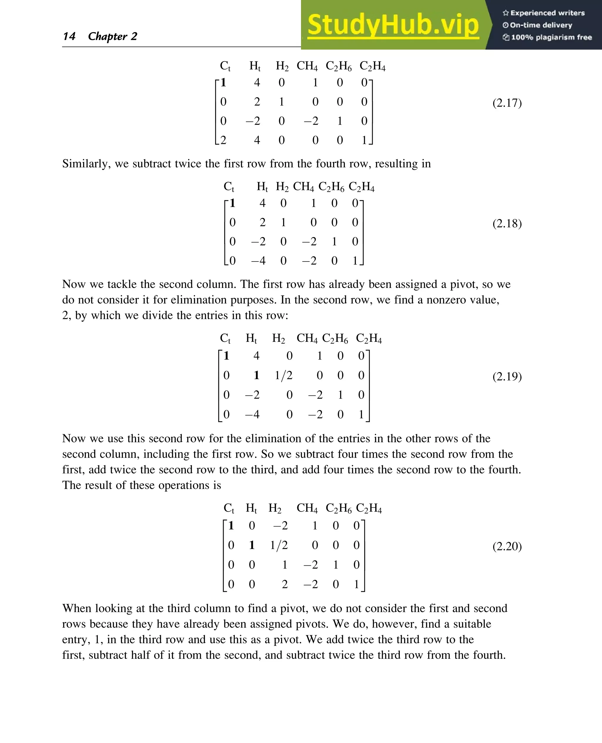
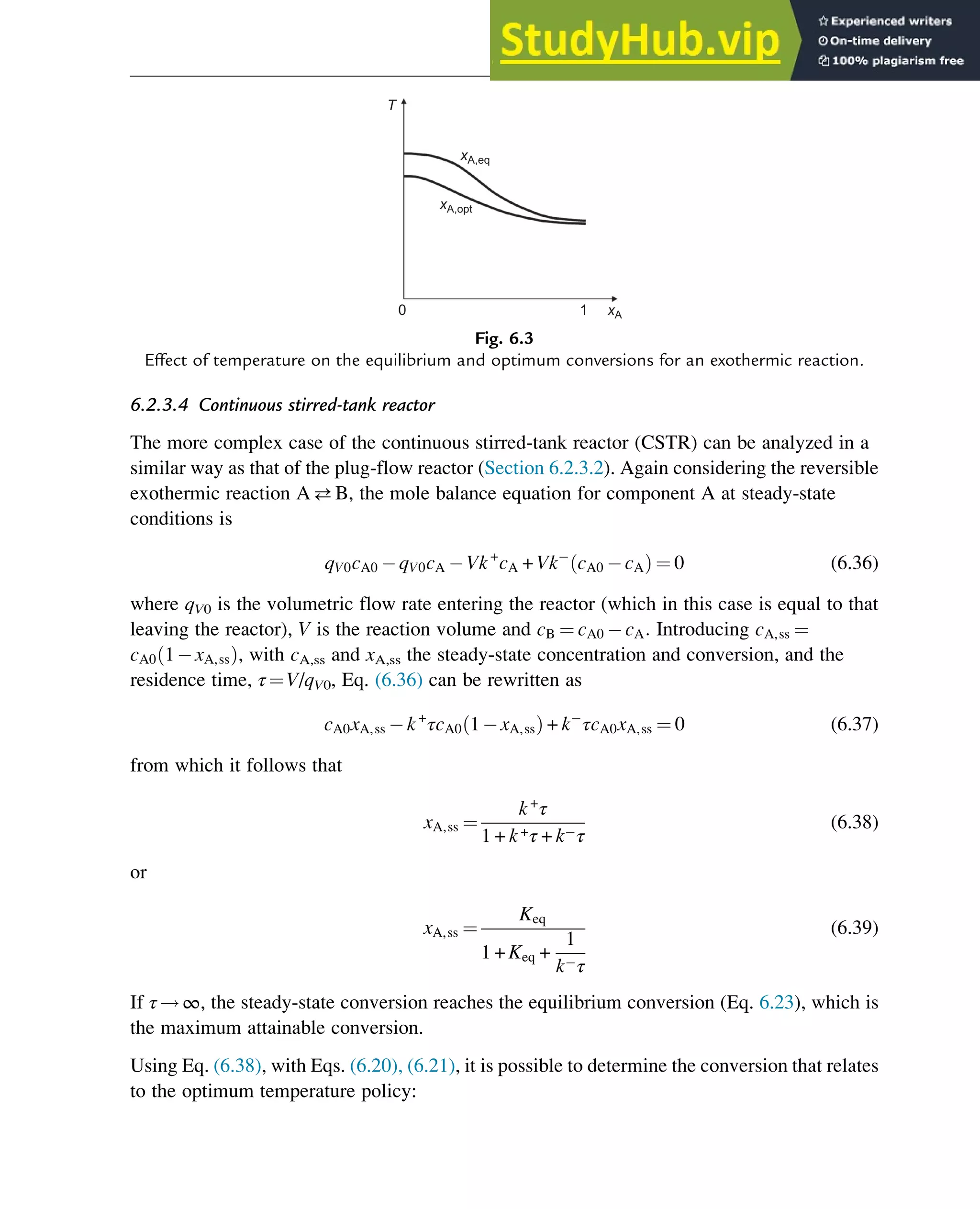
![f ¼ a[rowsdone][columnsdone]
g ¼ a[i][columnsdone]
# … this loop handles the linear combination
for j in range(n):
a[i][j] ¼ a[i][j] * f - a[rowsdone][j] * g
# … now we normalize the results by calculating their greatest common divisor, h
h ¼ 0
for j in range(n):
h ¼ fractions.gcd(h, a[i][j])
# … and if it is nonzero, divide by it
if h ! ¼ 0:
for j in range(n):
a[i][j] ¼ a[i][j] / h
# … this completes the work and we register the new row as being completed
rowsdone ¼ rowsdone + 1
Summarizing: the matrix is assumed to be given as a list of lists of integers. Its dimensions
m and n are obtained from this representation, and then the code successively inspects each
of the columns to see if it contains a pivot. Because all arithmetic is exact using the built-in
unlimited precision integers of Python, the greatest common divisor of every new row is
eliminated along the way. Whenever a pivot is found in a column, a new pivot row has
been found and the number of rows done is increased accordingly. Finally, the matrix a
has been modified to be in RREF form.
Nomenclature
Symbols
ai real number
ΔrHi enthalpy change of reaction i (J mol 1
)
Keq,i equilibrium coefficient of reaction i
M molecular matrix
mA column vector of atomic masses (kg mol 1
)
mM column of molar masses (kg mol 1
)
ni amount of component i (mol)
Chemical Composition and Structure: Linear Algebra 33](https://image.slidesharecdn.com/advanceddataanalysisandmodellinginchemicalengineering-230807160524-2b99ba17/75/Advanced-Data-Analysis-and-Modelling-in-Chemical-Engineering-pdf-39-2048.jpg)
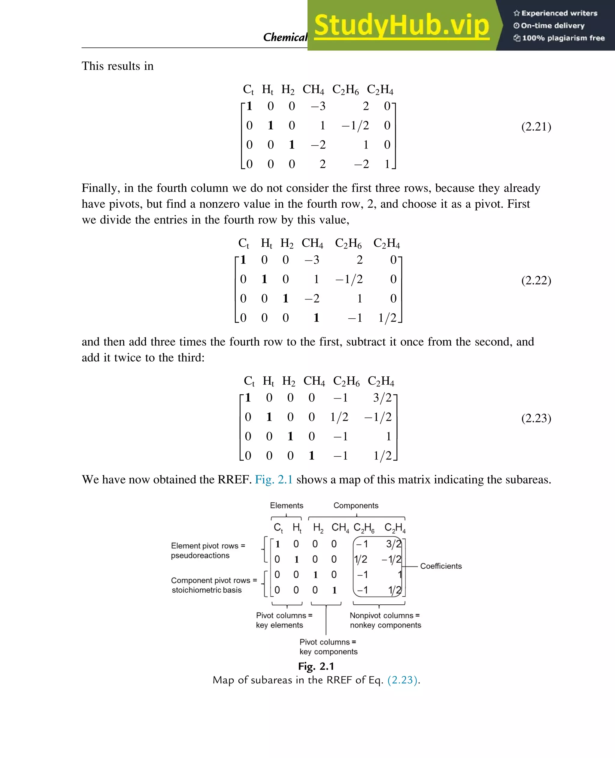
![solution of the original set of equations [x(t), yss(x(t))] at ε!0 approaches that of the
degenerated system uniformly on the segment [t0, tfinal]. The functions x(t) for the original and
degenerated systems approach each other uniformly throughout the segment [0, tfinal].
This statement can be presented qualitatively in a simpler way: The solution of the original
system approaches the solution of the degenerated system if the subsystem of fast motion
g
x,
y
ð Þ ¼ 0 has a stable solution and the initial conditions are “attracted” by this solution.
Different actual systems generate the small parameter ε in different ways. For example, in
homogeneous chain reactions, the small parameter is a ratio of rate coefficients. It arises
because the reactions in which free radicals, which are unstable and thus are short-lived,
participate are much faster than the other reactions.
In heterogeneous gas-solid catalytic systems, the small parameter is the ratio of the total amount
of surface intermediates nt,int to the total amount of reacting gas molecules nt,g present in the
reactor:
ε ¼
nt,int
nt,g
¼
ΓtScat
ctVg
(4.20)
with Γt the total concentration of surface intermediates, Scat the catalyst surface, ct the total
concentration of gas molecules, and Vg the gas volume.
In contrast to free radicals, surface intermediates may be relatively long-lived. Yablonskii et al.
(1991) have indicated different scenarios for reaching QSS regimes in such systems.
If ε!0 and the system of fast motion has a unique and asymptotically stable global steady state
at every fixed yi, we can apply Tikhonov’s theorem and, starting from a certain value of ε, use a
QSS approximation.
Summing up the theoretical analysis of the QSS problem, we can distinguish two types of
behavior:
• A QSS caused by a difference in kinetic parameters (rate-parametric QSS).
• A QSS caused by a difference in mass balances of species (mass-balance QSS), that is,
a large difference in mass balances between gaseous or liquid reactants and products on the
one side, and substrate-enzyme complexes or catalytic surface intermediates on the other.
An example of the rate-parametric QSS has been presented in Section 4.3.5 using the two-step
consecutive reaction (4.7), Aƒ
ƒ!
ƒ
ƒ
k+
1
k
1
Bƒ
ƒ!
k2
C. Many examples of the mass-balance QSS are
presented by Yablonskii et al. (1991), in particular for a typical two-step catalytic mechanism:
(1) A + ZAZ and (2) AZB + Z. See also the corresponding analysis in the excellent review
on asymptotology by Gorban et al. (2010).
Physicochemical Principles of Simplification of Complex Models 97](https://image.slidesharecdn.com/advanceddataanalysisandmodellinginchemicalengineering-230807160524-2b99ba17/75/Advanced-Data-Analysis-and-Modelling-in-Chemical-Engineering-pdf-103-2048.jpg)


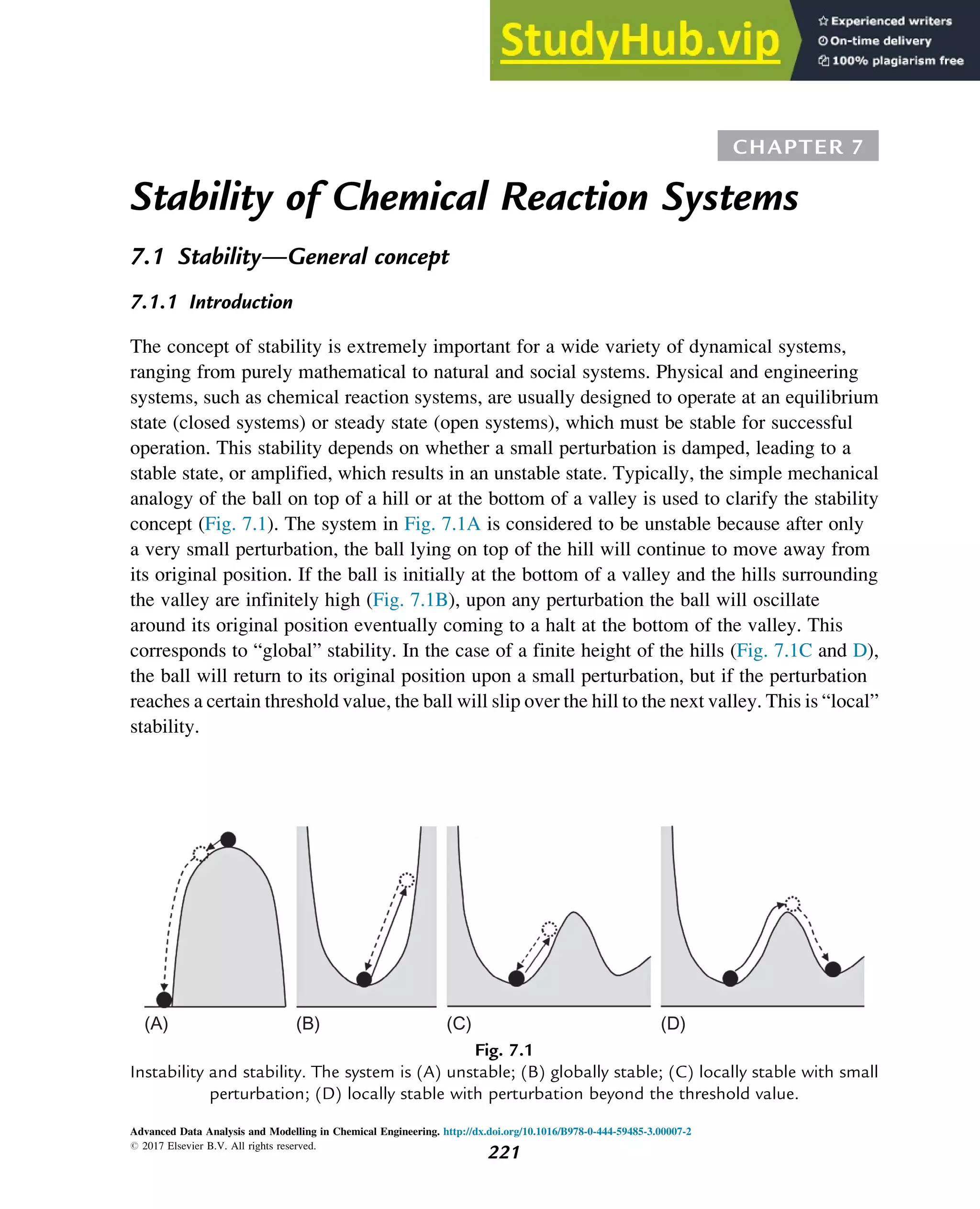
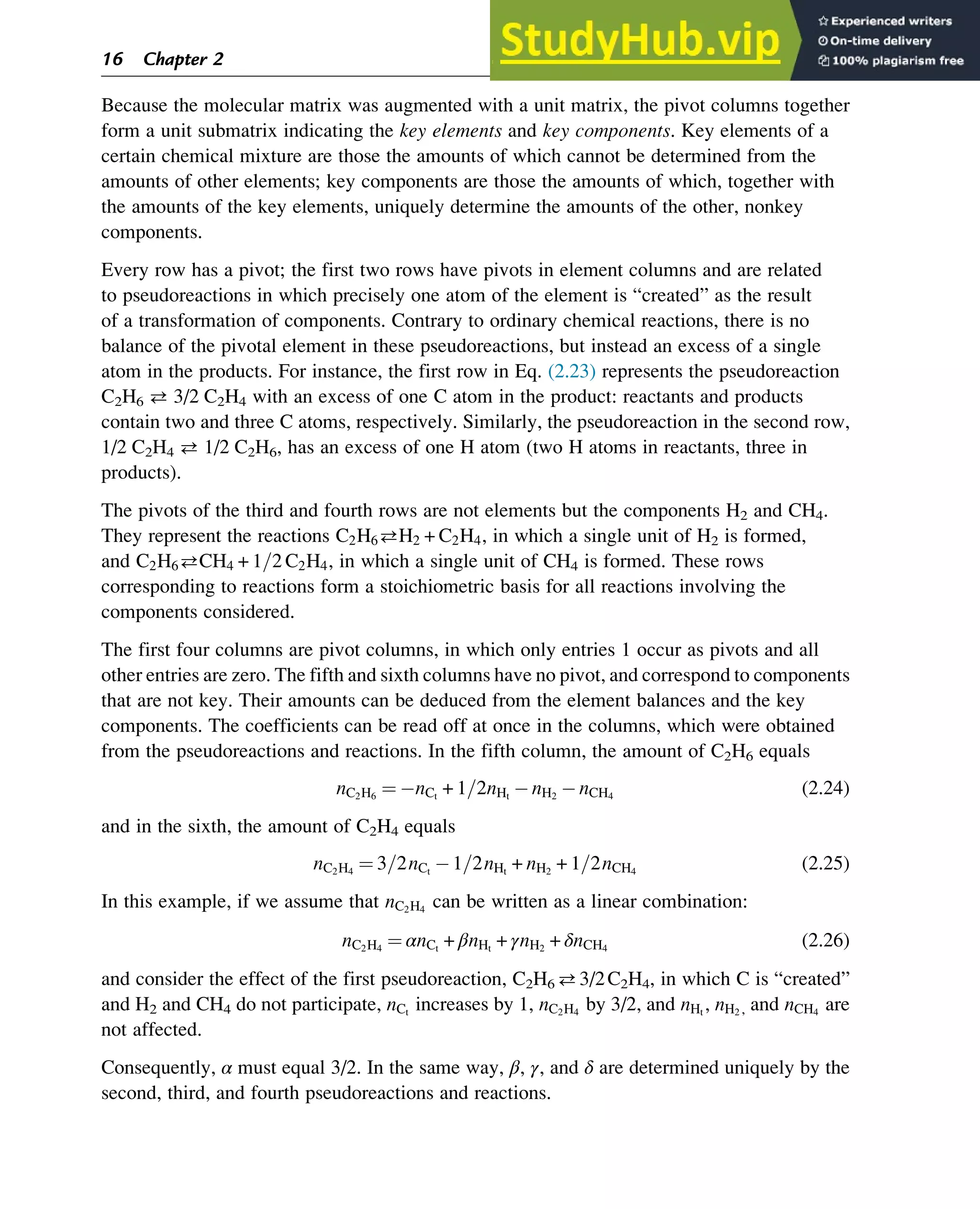
![7.1.2 Non-Steady-State Models
The dynamic behavior of chemical reaction systems is described in terms of non-steady-state
models, which in their simplest form are sets of ordinary differential equations of the type
dc
dt
¼ f c, k
ð Þ (7.1)
in which c is a vector of concentrations and k is a vector of kinetic parameters. The space of
vectors c is the phase space of Eq. (7.1), the space in which all possible states of the
reaction system are represented with every possible state corresponding to one unique point.
The points are specified by the state variables c1,c2,…,cNc
, where Nc is the number of
components present in the chemical reaction mixture. In the case of a nonisothermal system,
this set of equations has to be supplemented with an equation of the type
dT
dt
¼ f c, k, h
ð Þ (7.2)
where h are heat parameters of the model, that is, heat capacities, heat-transfer coefficients, and
heats of reaction.
Eq. (7.1) has only one solution, c(t, k, c0), for any nonnegative initial condition c(0, k, c0)¼c0,
which is natural for chemical kinetics. The changing state of the system with time traces a
path c(t, k, c0) at fixed k and c0 and t 2 [0, 1] through the phase space and is called a phase
trajectory. A phase trajectory represents the set of chemical compositions of the reaction
mixture that can be reached from a particular initial condition.
From a physicochemical point of view, we are only interested in positive trajectories, which in
mathematics are called “semitrajectories.” However, in some cases, values of c(t, k, c0) on
negative trajectories with t 2 [ 1, 0] and whole trajectories with t 2 [ 1,1] are informative
regarding the behavior in the physicochemically relevant (positive) concentration domain.
As Eq. (7.1) for each initial condition has only one, unique solution, every point in the phase
space is passed by one and only one of the phase trajectories, which neither cross one another
nor merge.
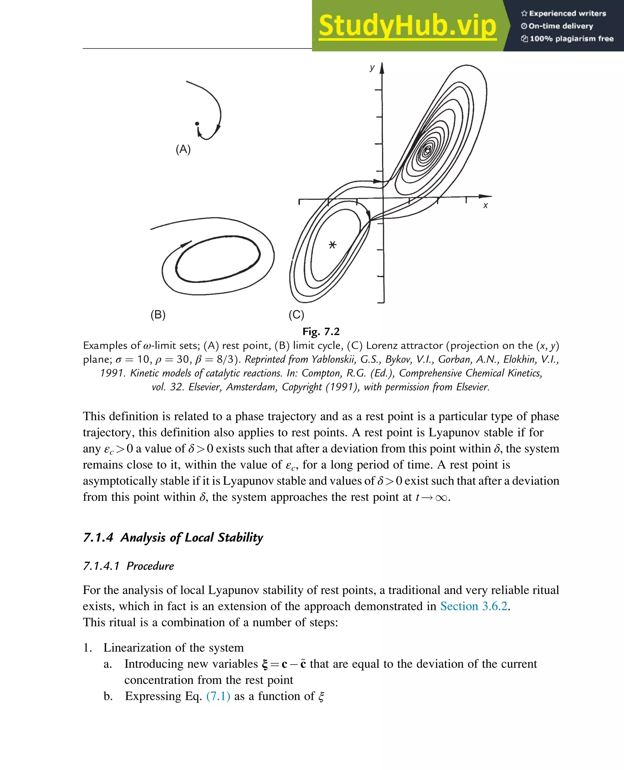
A family of phase trajectories starting from different initial states is called a phase diagram or
phase portrait. A phase portrait graphically shows how the system moves from the initial
states and reveals important aspects of the dynamics of the system. Certain phase portraits
display one or more attractors, which are long-term stable sets of states toward which a system
tends to evolve (is attracted) dynamically, from a wide variety of initial conditions,
the basin of attraction. The simplest type of attractor is a so-called rest point. This is a
point for which the derivatives of all the state variables are zero:
dc
dt
¼ f c, k
ð Þ ¼ 0 (7.3)
222 Chapter 7](https://image.slidesharecdn.com/advanceddataanalysisandmodellinginchemicalengineering-230807160524-2b99ba17/75/Advanced-Data-Analysis-and-Modelling-in-Chemical-Engineering-pdf-226-2048.jpg)
![sum p+q3. These results are based on the algebraic analysis of the number of positive roots
in the interval [0,1] using Descartes’s rule of signs and Sturm’s theorem.
The main result is that real multiplicity of steady states—the existence of two internal stable
steady states and one internal unstable steady state—can be explained using one of the four
mechanisms shown in Table 7.3. If the experimentally observed steady-state reaction rate is
characterized by two different branches, and multiplicity of steady states is observed, one of
these four mechanisms can be used to interpret the data. We prefer to use mechanism B because
its steps are characterized by overall reaction orders that are not larger than two. In fact, this
mechanism is identical to the mechanism represented by Eq. (7.102), an example of which is
the adsorption mechanism for the oxidation of carbon monoxide (Eq. (7.103)). We will return
to this mechanism in Chapter 11, in which the problem of critical simplification is discussed.
7.5 Chemical Oscillations in Isothermal Systems
7.5.1 Historical Background
The discovery of isothermal chemical oscillations was one of the big scientific sensations of the
20th century. Belousov and Zhabotinsky found self-sustained oscillations in the cerium-ion
catalyzed oxidation of citric acid by bromate, now known as the Belousov-Zhabotinsky
reaction. This reaction became one of the starting points for Prigogine and his coworkers in
Brussels for studying complicated dynamic behavior of chemical mixtures that are far from
equilibrium (Prigogine and Lefever, 1968; Glansdorff and Prigogine, 1971; Nicolis and
Prigogine, 1977). They used a model with a specific type of mechanism involving autocatalytic
reactions, later named the Brusselator, for the quantitative interpretation of chemical
oscillations in isothermal systems. An autocatalytic reaction is a reaction in which at least one
of the reactants is also a product, for example, A+B!2 A. Prigogine received the 1977 Nobel
Prize in Chemistry for this work. In the early 1970s, the research by Prigogine’s group inspired
Table 7.3 Adsorption mechanisms that can explain the multiplicity of steady states
A (1) A + ZAZ
(2) B + ZBZ
(3) 2AZ + BZ ! A2B + 3Z
B (1) A2 + 2Z2AZ
(2) B + ZBZ
(3) AZ + BZ ! AB + 2Z
C (1) A2 + 2Z2AZ
(2) B + ZBZ
(3) 2AZ + BZ ! A2B + 3Z
D (1) A2 + 2Z2AZ
(2) B + ZBZ
(3) AZ + 2BZ ! AB2 + 3Z
Stability of Chemical Reaction Systems 251](https://image.slidesharecdn.com/advanceddataanalysisandmodellinginchemicalengineering-230807160524-2b99ba17/75/Advanced-Data-Analysis-and-Modelling-in-Chemical-Engineering-pdf-255-2048.jpg)
![The reduced set of equations for the time derivatives of θAZ and θBZ, Eqs. (7.123) and (7.124),
with not three but two variables, in which θ(BZ)* is regarded as a parameter, is a catalytic
trigger. For this system, a unique steady state is stable. If there are three steady states, the two
outer steady states are stable and the middle steady state is unstable.
The complete set of equations with three variables, Eqs. (7.123)–(7.125), including the
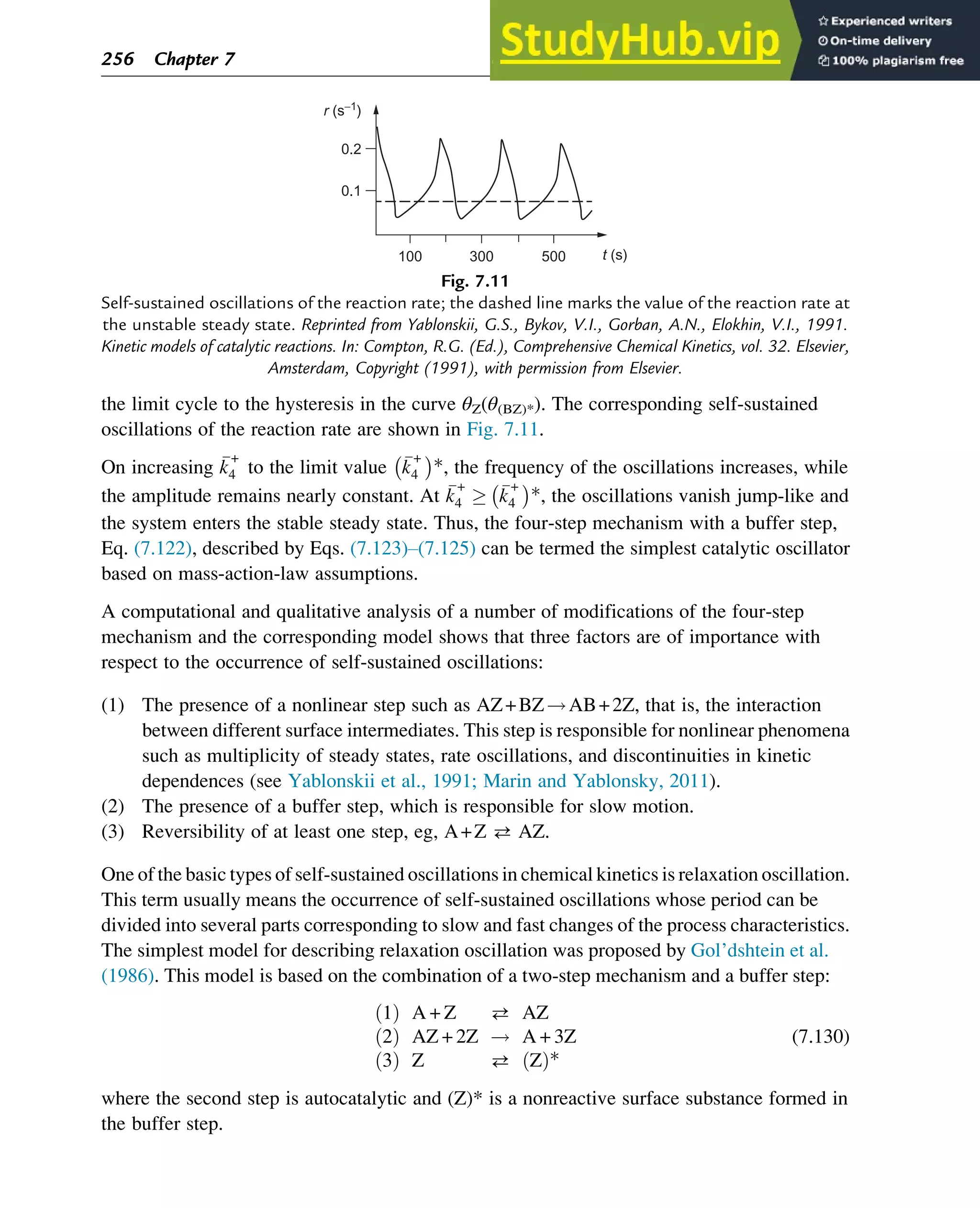
buffer step, may have a unique unstable solution. In view of the Poincaré-Bendixson theorem,
this is a necessary and sufficient condition for the occurrence of oscillations. For this set of
equations, the solution is considered to be in the so-called reaction simplex S:
S θAZ, θBZ, θ BZ
ð Þ* : θAZ 0, θBZ 0, θ BZ
ð Þ* 0, θAZ + θBZ + θ BZ
ð Þ* 1 (7.128)
Let θAZ,ss, θBZ,ss, θ BZ
ð Þ*,ss ¼ θss
ð Þ be the steady-state solution of the set of equations,
Eqs. (7.123)–(7.125). For this system, the characteristic equation is
λ3
+ σλ2
+ δλ + Δ ¼ 0 (7.129)
where σ ¼ Tr(J), δ¼a11 +a22 +a33 ¼Tr(adjJ), and Δ¼ det J. J¼[aij] (i, j¼1, 2, 3) is
the matrix of the corresponding linearized set of equations at the steady state; a11, a22, and a33 are
the principal minors of matrix J; and adjJ is the adjoint of J. The values of the nonpositive
roots λ1 and λ2 of matrix J are determined by the relationship between σ, δ, and Δ, with σ 0.
It can be shown (Yablonskii et al., 1991) that a necessary and sufficient condition for the
instability of the steady state is that δ is negative. For δ¼0, the parameters are at their critical
values, that is, the value for which the real parts of the characteristic roots λ1 and λ2 change sign.
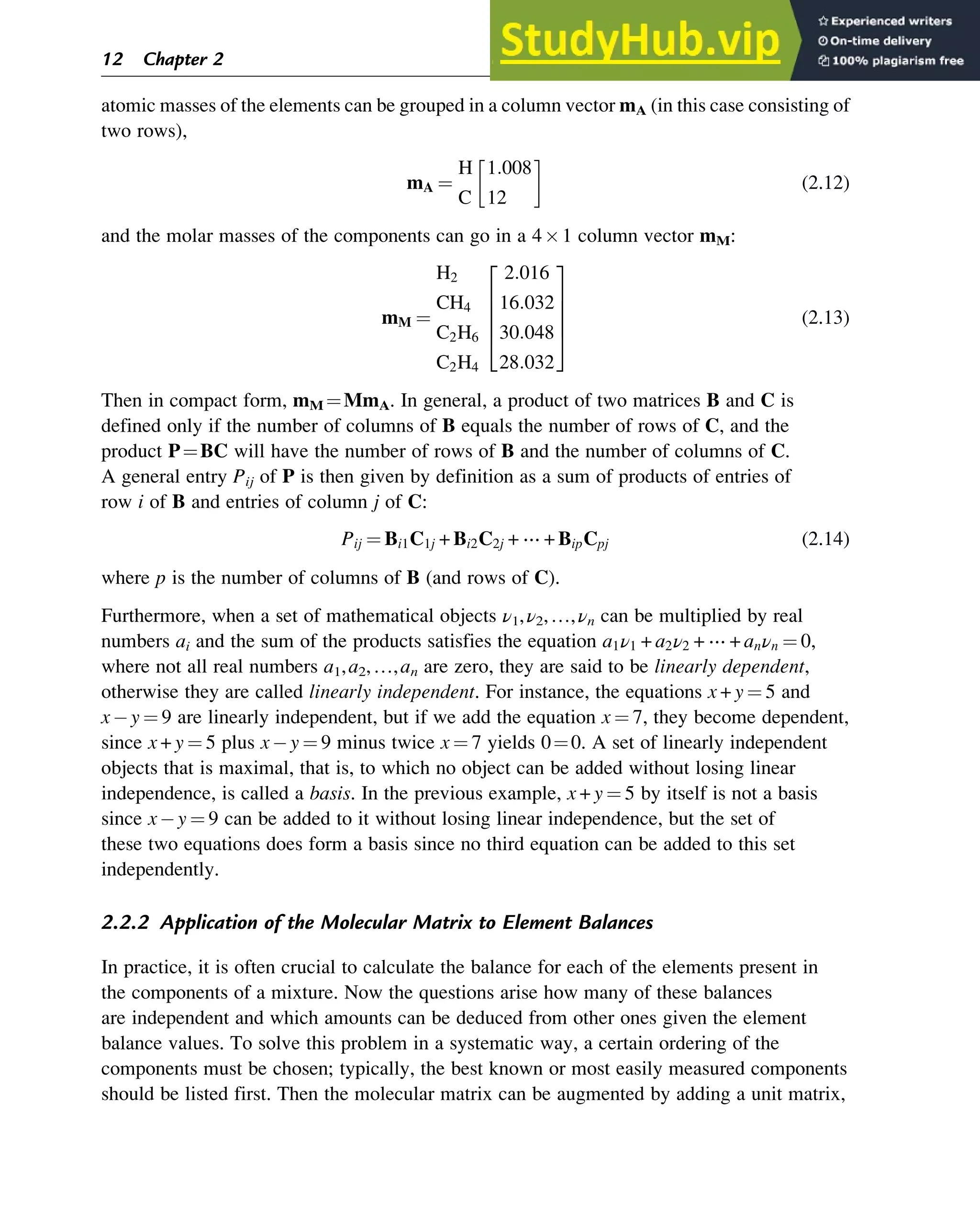
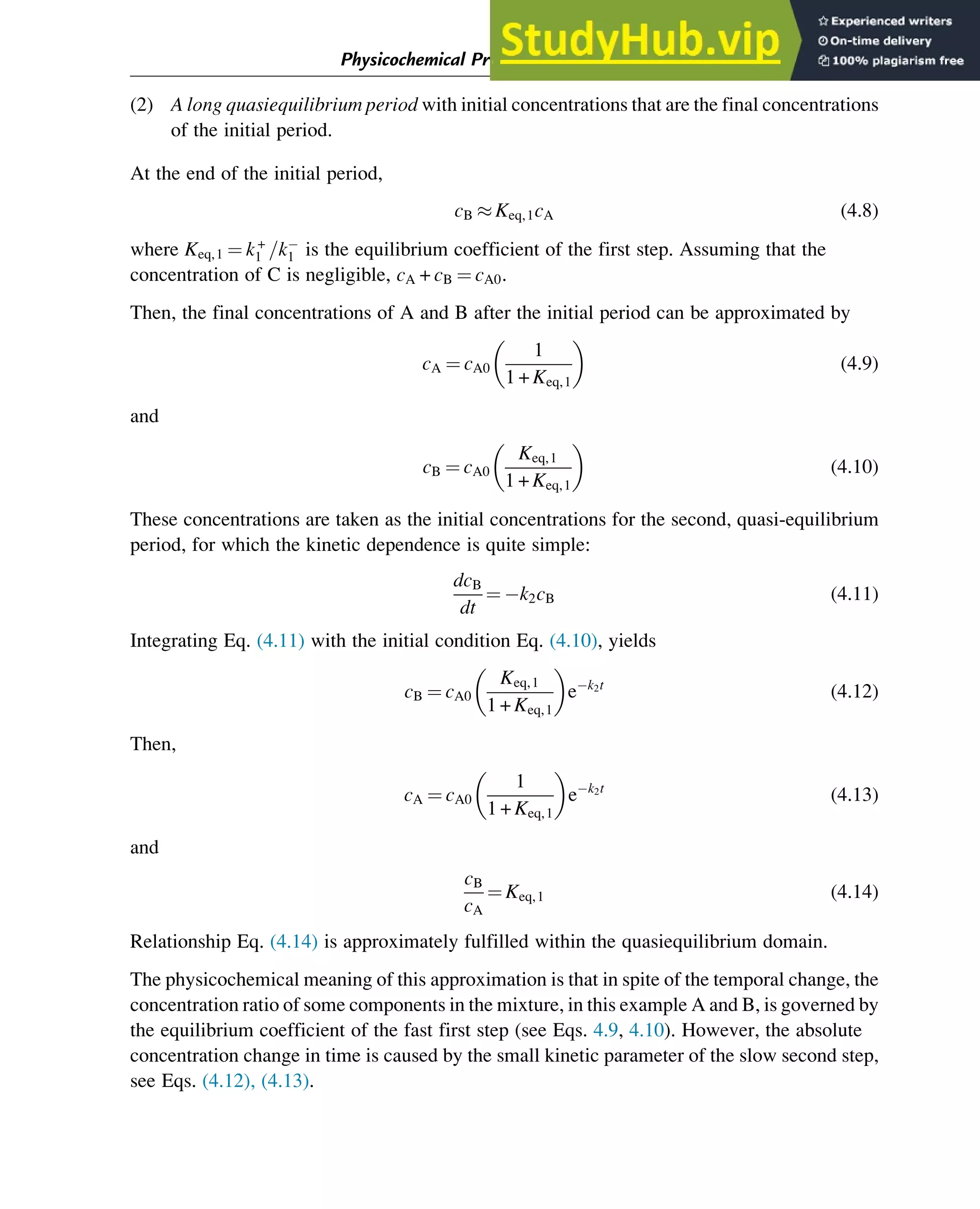
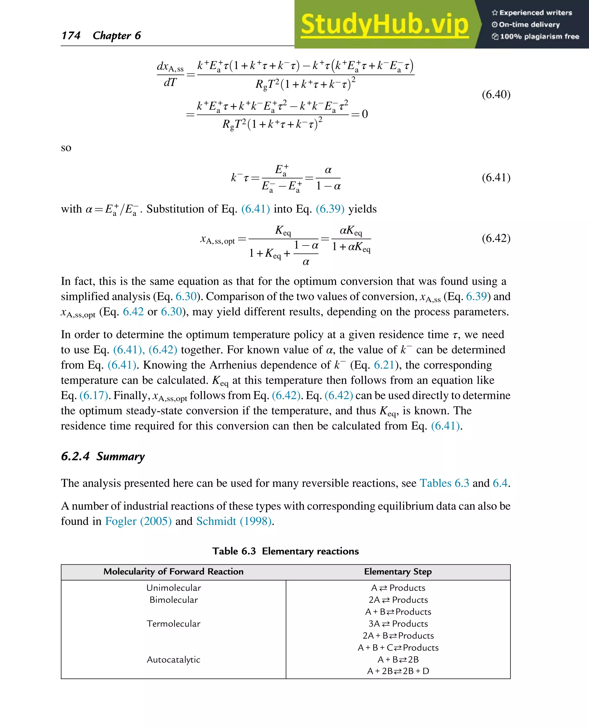
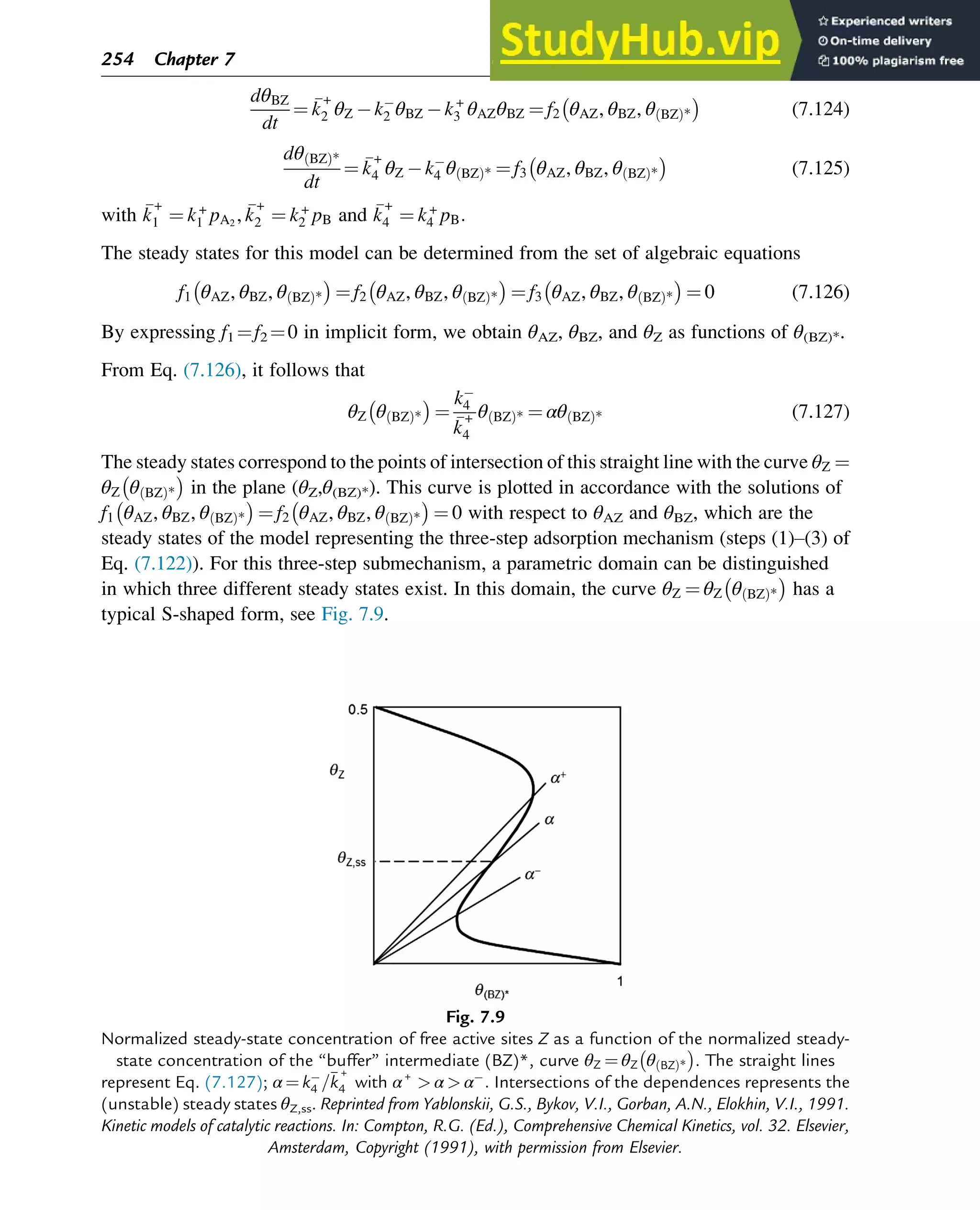
When the parameters for reaction steps (1)–(3) are properly chosen, a parametric domain
for step (4) can be found that results in a unique unstable steady state, resulting in oscillation
(see Fig. 7.10). Comparison with Fig. 7.9 shows that the oscillations are observed in the
domain close to the hysteresis in the curve θZ(θ(BZ)*). The shape of the limit cycles in Fig. 7.10
very much depends on the values of
k
+
4 and k4 . The lower these values, the closer the shape of
0.3
(A) (B)
0
0.1
0.2
0.3
0.5 0.7 0.3
0.3
0.5
0.7
0.5
q(BZ)* q(BZ)*
qAZ
qZ
Fig. 7.10
Examples of limit cycles on (A) (θ(BZ)*, θZ) and (B) (θ(BZ)*, θAZ) phase-space projections. Reprinted from
Yablonskii, G.S., Bykov, V.I., Gorban, A.N., Elokhin, V.I., 1991. Kinetic models of catalytic reactions. In: Compton,
R.G. (Ed.), Comprehensive Chemical Kinetics, vol. 32. Elsevier, Amsterdam, Copyright (1991), with permission
from Elsevier.
Stability of Chemical Reaction Systems 255](https://image.slidesharecdn.com/advanceddataanalysisandmodellinginchemicalengineering-230807160524-2b99ba17/75/Advanced-Data-Analysis-and-Modelling-in-Chemical-Engineering-pdf-259-2048.jpg)

![xs ¼
X
i
is
Ri
½ Š + Pi
½ Š
ð Þ
X
i
is 1
Ri
½ Š + Pi
½ Š
ð Þ
(10.1)
in which [Ri] is the concentration of living polymer molecules with chain length i, and [Pi]
is the concentration of dead polymer molecules with chain length i. The calculation is
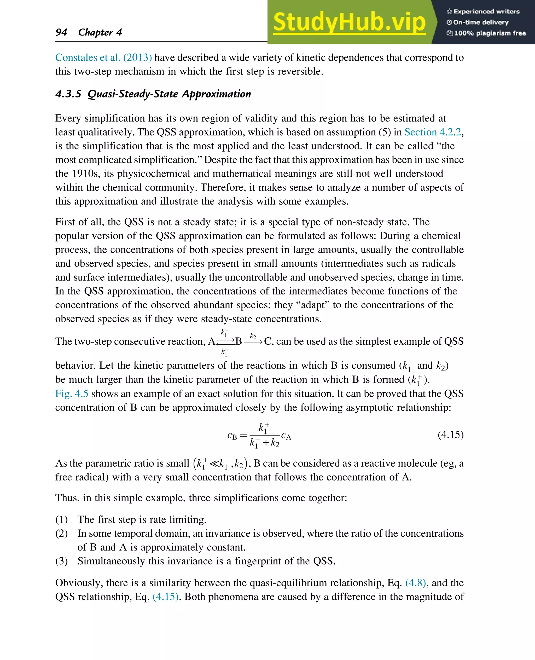
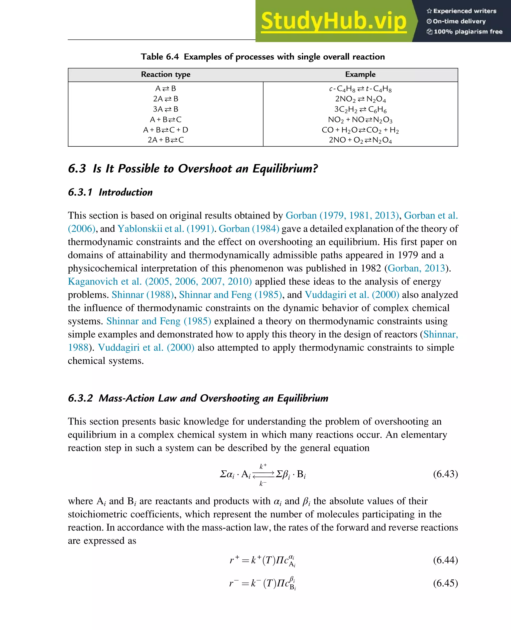
typically limited to the first, second, and third average (x1, x2, and x3). These first three averages
are also known as the number-, mass-, and z-average chain length (xn/m/z), as illustrated in
Fig. 10.4.
The relative position of these three averages allows assessment of the broadness of the CLD
without its explicit calculation:
Dn ¼
xm
xn
(10.2)
Dm ¼
xz
xm
(10.3)
For values of Dn and Dm close to one, the CLD is narrow, whereas for values higher than 1.5, the
CLD is classified as broad. Typically only Dn, referred to as the polydispersity index or
dispersity, is used as a measure of the broadness of the CLD (Gilbert et al., 2009).
From Eq. (10.1), it follows that to calculate xs (s¼1, 2, 3), the following moments (0s0
3)
have to be known:
λs0 ¼
X
i
is0
Ri
½ Š (10.4)
0.1
0.08
0.06
0.04
0.02
0
0 20 40
Chain length (–)
Number
fraction
(–)
60 80 100
Fig. 10.4
Representation of the number CLD (diamonds) via three averages (Eq. 10.1); s¼1, 2, 3 or n, m, z
(squares; left to right); simplified case of a maximum chain length of 100.
Polymers: Design and Production 311](https://image.slidesharecdn.com/advanceddataanalysisandmodellinginchemicalengineering-230807160524-2b99ba17/75/Advanced-Data-Analysis-and-Modelling-in-Chemical-Engineering-pdf-314-2048.jpg)
![dλs0
dt
¼ k3λ0λs0 + k2 M
½ Š R0
½ Š +
k2 M
½ Šλ0 s0
¼ 1
ð Þ
k2 M
½ Šλ0 + 2k2 M
½ Šλ1 s0
¼ 2
ð Þ
k2 M
½ Šλ0 + 3k2 M
½ Šλ1 + 3k2 M
½ Šλ2 s0
¼ 3
ð Þ
8
:
(10.8)
dμs0
dt
¼ k3λ0λs0 (10.9)
d M
½ Š
dt
¼ k2 M
½ Š R0
½ Š k2 M
½ Šλ0 (10.10)
d R0
½ Š
dt
¼ 2k1 I2
½ Š k2 M
½ Š R0
½ Š (10.11)
In these equations, only [M] and [I2] have a nonzero value at t¼0. In particular, Eq. (10.10)
allows for the calculation of the monomer conversion profile without the interference of
higher order moments.
In case the reactions in Scheme 10.1 are assumed to be dependent on the chain length, k2 and k3
have to be replaced by population-weighted rate coefficients defined as
k2,s ¼
X
i
is
k2,i Ri
½ Š
X
i
is
Ri
½ Š
(10.12)
k3,s ¼
X
i,j
is
k3,ij Ri
½ Š Rj
X
i,j
is
Ri
½ Š Rj
(10.13)
in which k2,i and k3,ij are the corresponding (apparent) chain length dependent rate coefficients
(with k3,ij ¼2k3a,ij). However, in the classical method of moments, no assessment of the
individual concentrations of the living macromolecules is performed and the dependency on the
chain length is either ignored or the population-weighted rate coefficients are calculated
based on overall polymerization characteristics (eg, the polymer mass fraction).
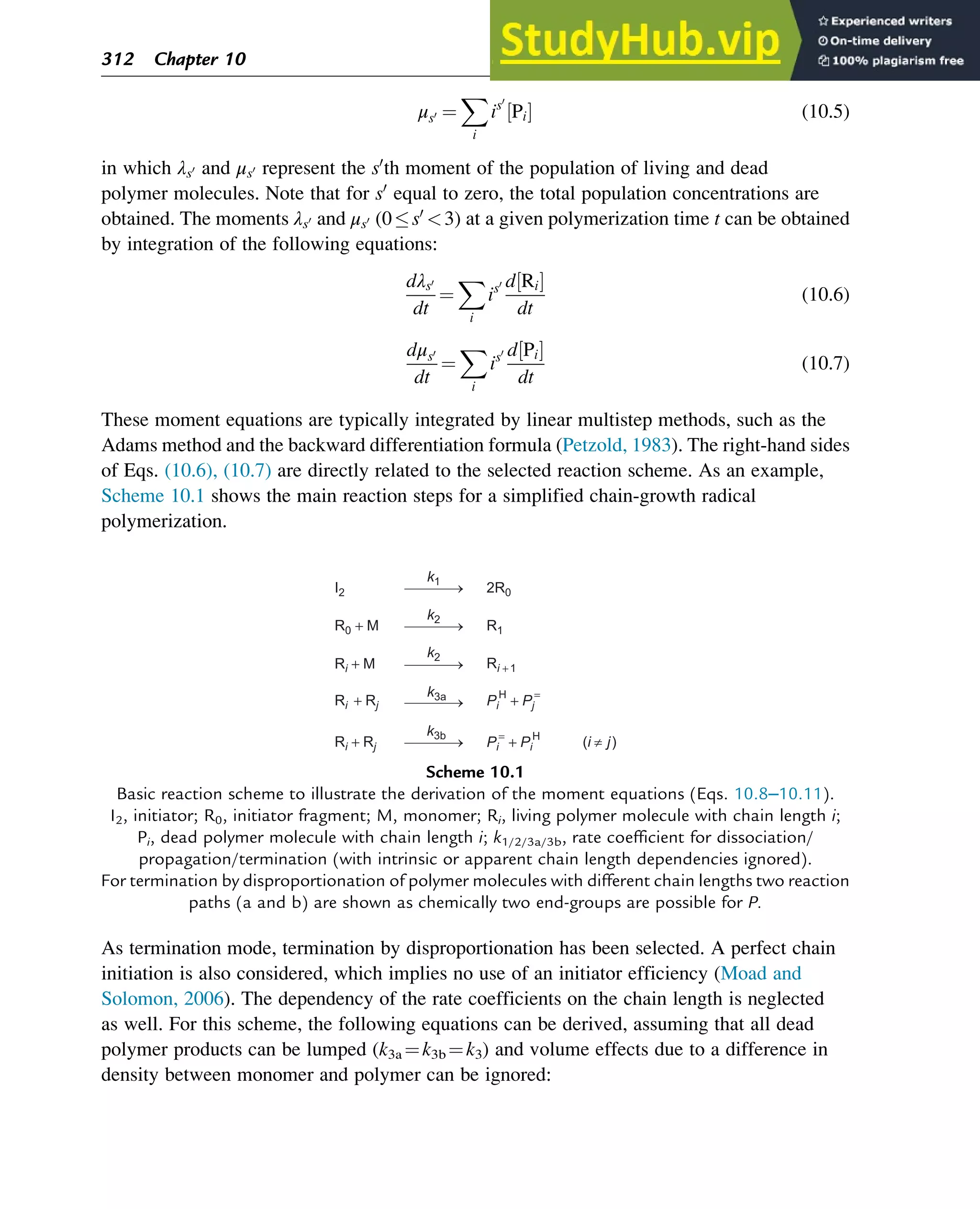
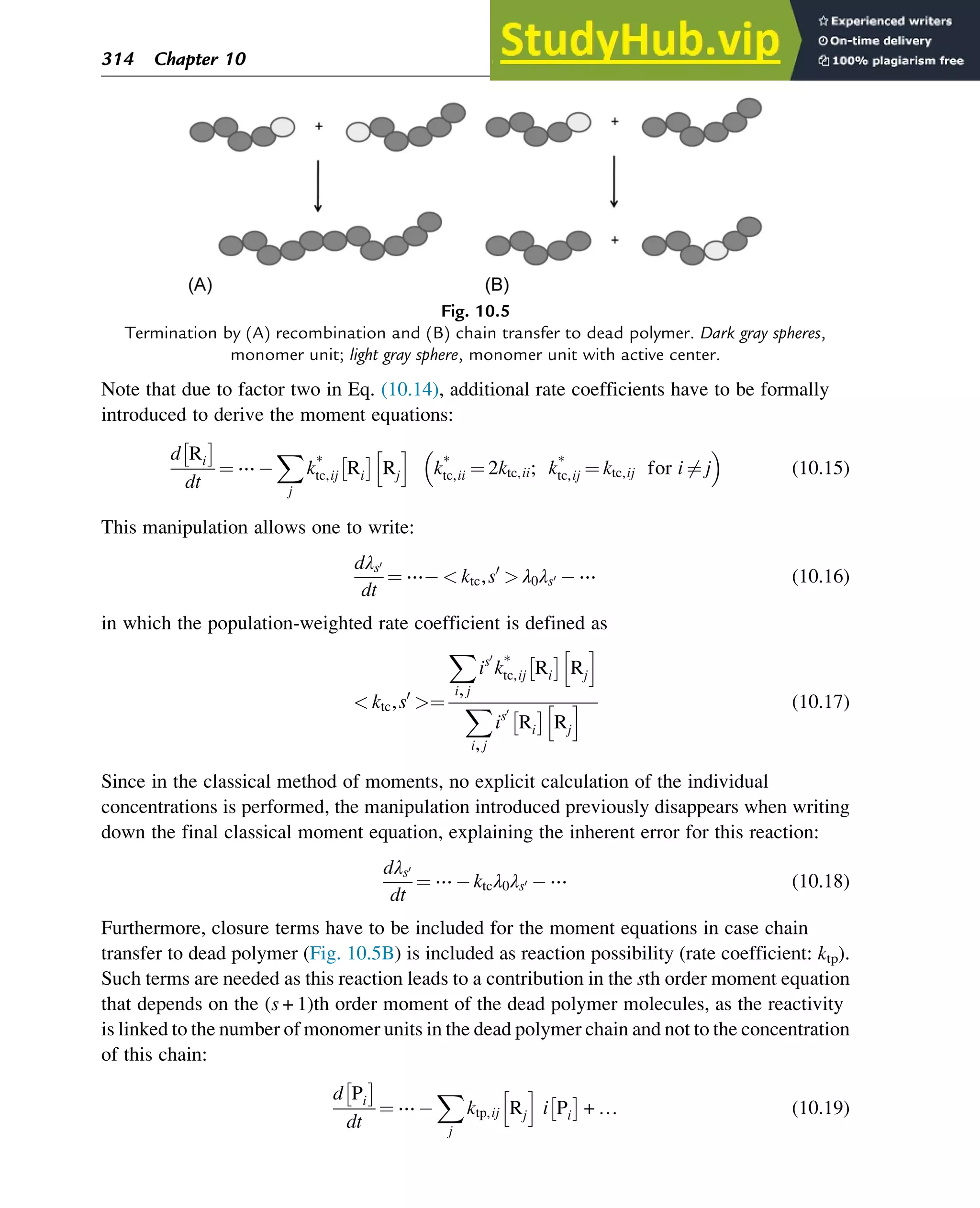
It should be noted that for termination by recombination (Fig. 10.5A), inherently an error is
introduced regarding its contribution in the classical moment equations. For the individual
living polymer continuity equations, it can be derived that the contribution of termination by
recombination is
d Ri
½ Š
dt
¼ ⋯ 2ktc,ii Ri
½ Š2
X
j i6¼j
ð Þ
ktc,ij Ri
½ Š Rj
(10.14)
in which ktc,ii and ktc,ij (i6¼j) are the homo- and cross-termination rate coefficients.
Polymers: Design and Production 313](https://image.slidesharecdn.com/advanceddataanalysisandmodellinginchemicalengineering-230807160524-2b99ba17/75/Advanced-Data-Analysis-and-Modelling-in-Chemical-Engineering-pdf-316-2048.jpg)
![p1 ¼
μ2
μ0
0:5
exp σ2
¼
μ0μ2
μ1
2
(10.24)
A more advanced method is the inverse (discrete) Laplace transformation (or probability
generating function [pgf]) method (Asteasuain et al., 2002a,b, 2004). In this method, the
CLD is reconstructed from the integrated moment equations, as illustrated in Fig. 10.6.
A number and mass probability are first introduced for the living polymer molecules:
P0,R i
ð Þ ¼
Ri
λ0
(10.25)
P1,R i
ð Þ ¼
i Ri
λ1
(10.26)
Similarly, for the dead polymer molecules, a number and mass probability are defined
P0,P i
ð Þ ¼
Pi
μ0
(10.27)
Fig. 10.6
Principle of Laplace transformations (or probability generating function (pgf) method) to reconstruct
the CLD based on the moment equations. k, vector with rate coefficients; [A], vector with
concentrations of nonmacromolecules; Δt, time step for integration; CLD, chain length distribution;
G, transformed z-variable.
316 Chapter 10](https://image.slidesharecdn.com/advanceddataanalysisandmodellinginchemicalengineering-230807160524-2b99ba17/75/Advanced-Data-Analysis-and-Modelling-in-Chemical-Engineering-pdf-319-2048.jpg)
![between the averages of the CLD as obtained with these “correct” moment equations using
fixed but updated population-weighted apparent rate coefficients per time step and the averages
as obtained based on the reconstructed CLD in a parallel solver. In this parallel solver, for the
calculation of the concentrations of part of the individual species, the QSSA is applied and an
iterative solution strategy is selected. In particular, for controlled radical polymerizations
(CRP), this method has proven to be successful. Fig. 10.7 shows the principle of this solution
strategy for an important CRP process, namely nitroxide-mediated polymerization (NMP;
Scheme 10.2; Malmström and Hawker, 1998).
Fig. 10.7
Principle of the extended method of moments applied for NMP using “correct” moment
equations (solver 1) and requiring convergence for the resulting CLD averages and those obtained via
iterative integration of the set of differential algebraic equations using the QSSA for the living
species and keeping the continuity equations for the dormant macrospecies (solver 2). [A], vector
with concentrations of nonmacromolecules; [C]: vector with all concentrations; k, vector
with population-weighted (apparent) rate coefficients; k, vector with all individual (apparent)
rate coefficients; kA, vector with all (apparent) rate coefficients for reactions involving only
nonmacromolecules; f and g, functions; Δt, time step for the integration (Bentein et al., 2011).
318 Chapter 10](https://image.slidesharecdn.com/advanceddataanalysisandmodellinginchemicalengineering-230807160524-2b99ba17/75/Advanced-Data-Analysis-and-Modelling-in-Chemical-Engineering-pdf-321-2048.jpg)
![chosen to be of a different size (Butté et al., 2002; Kumar and Ramkrishna, 1996). Typically the
size variation is of a logarithmic nature in order to accurately capture the contributions of
macrospecies with a small chain length.
Each interval Nk (k¼1,…, Nmax) is characterized by only one chain length belonging to
that interval, that is, the characteristic chain length or pivot ik (see Fig. 10.8). In other words, the
total concentration of, for example, dead polymer molecules in Nk is the product of the
concentration of dead polymer molecules with that particular chain length and the interval size
Δk. The continuity equations are integrated only per interval leading to an overall reduction of
the number of equations to be considered. For the living and dead polymer molecules, the
symbols [Rk
*] and [Pk
*] (k¼1,…, Nmax) are typically used to denote the corresponding overall
concentrations.
In the simplest case, chain transfer to the monomer (Scheme 10.3, rate coefficient: ktrM) is
considered and a contribution to the continuity equation for [Rk
*] can be derived directly, as the
reactants and products belong to the same interval:
d R*
k
dt
¼ ktrM R*
k
h i
M
½ Š + … (10.36)
However, for certain reactions only particular chain lengths belonging to other intervals
contribute to the population balance for a given interval. For example, for a product of
termination by recombination belonging to the interval k, the macroradical chain lengths im
and il (with m and l the corresponding intervals) have to be identified and a reverse lever
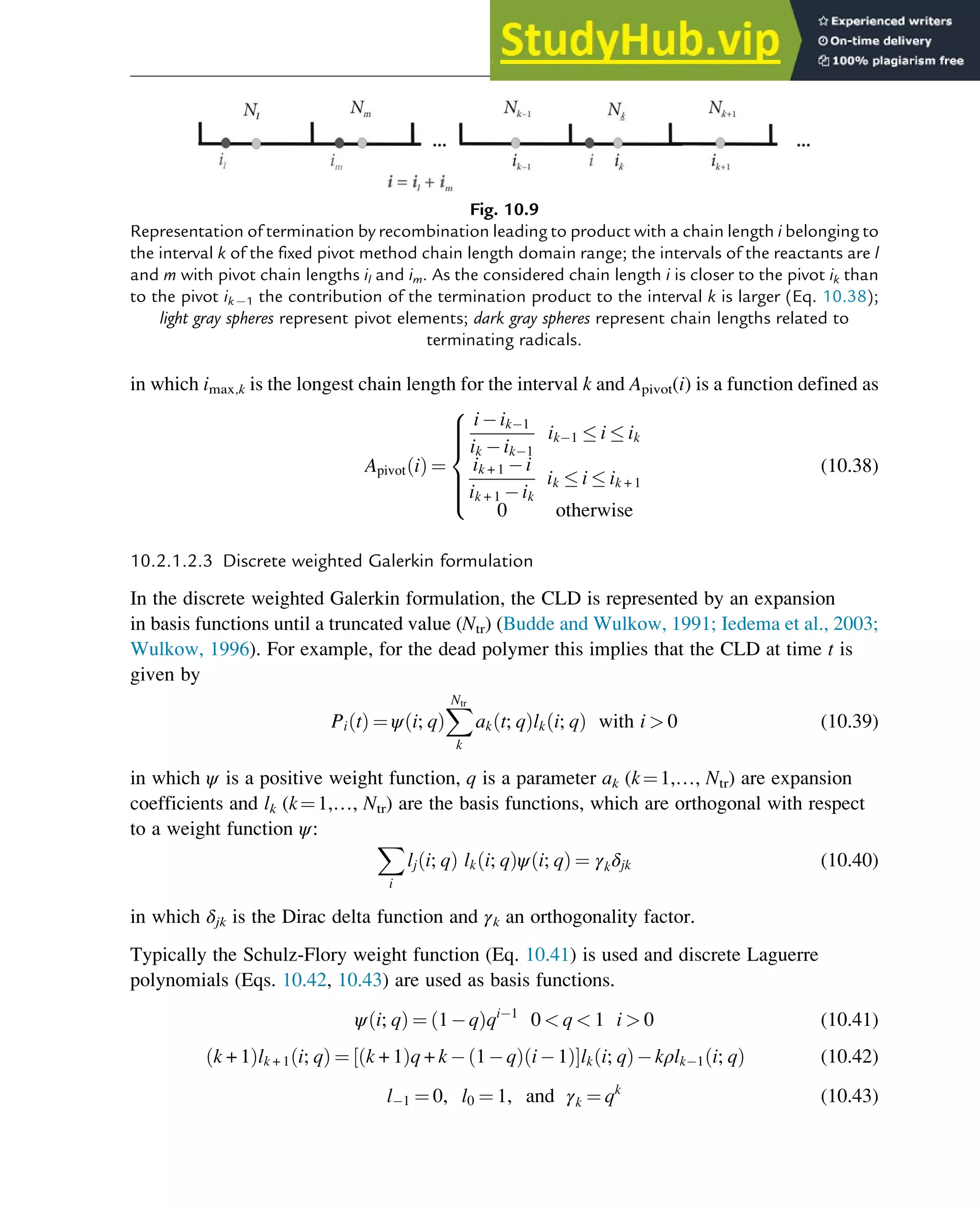
rule has to be applied (cf. Fig. 10.9):
d P*
k
dt
¼ … + ktc
X
imax,k
i¼1
X
il + im¼i
il¼1
Apivot i
ð Þ
R*
m
Δm
R*
l
Δl
(10.37)
Ri + M Pi + R0
ktrM
Scheme 10.3
Chain transfer to monomer.
Fig. 10.8
Division of the chain length range for the fixed pivot method; each interval can be of a
different size (Δk) but the sizes are fixed during the integration; typically a logarithmic scale is used; gray
spheres represent the pivot elements.
320 Chapter 10](https://image.slidesharecdn.com/advanceddataanalysisandmodellinginchemicalengineering-230807160524-2b99ba17/75/Advanced-Data-Analysis-and-Modelling-in-Chemical-Engineering-pdf-323-2048.jpg)
![The expansion coefficients are determined via substitution and application of the
orthogonality relation. For example, if the time dependency of the polymerization kinetics
(denoted here with 0
) can be described by
Pi
0
t
ð Þ ¼ B0
Pi t
ð Þ (10.44)
with B0
a representative matrix, it can be derived (Budde and Wulkow, 1991) that
γja0
j t
ð Þ ¼ Ψ i
ð Þ
X
k
aki t
ð Þ lj,B0
lk
(10.45)
with the inner product of two functions f and g defined as
f, g
ð Þ ¼
X
i
f i
ð Þg i
ð Þψ i
ð Þ (10.46)
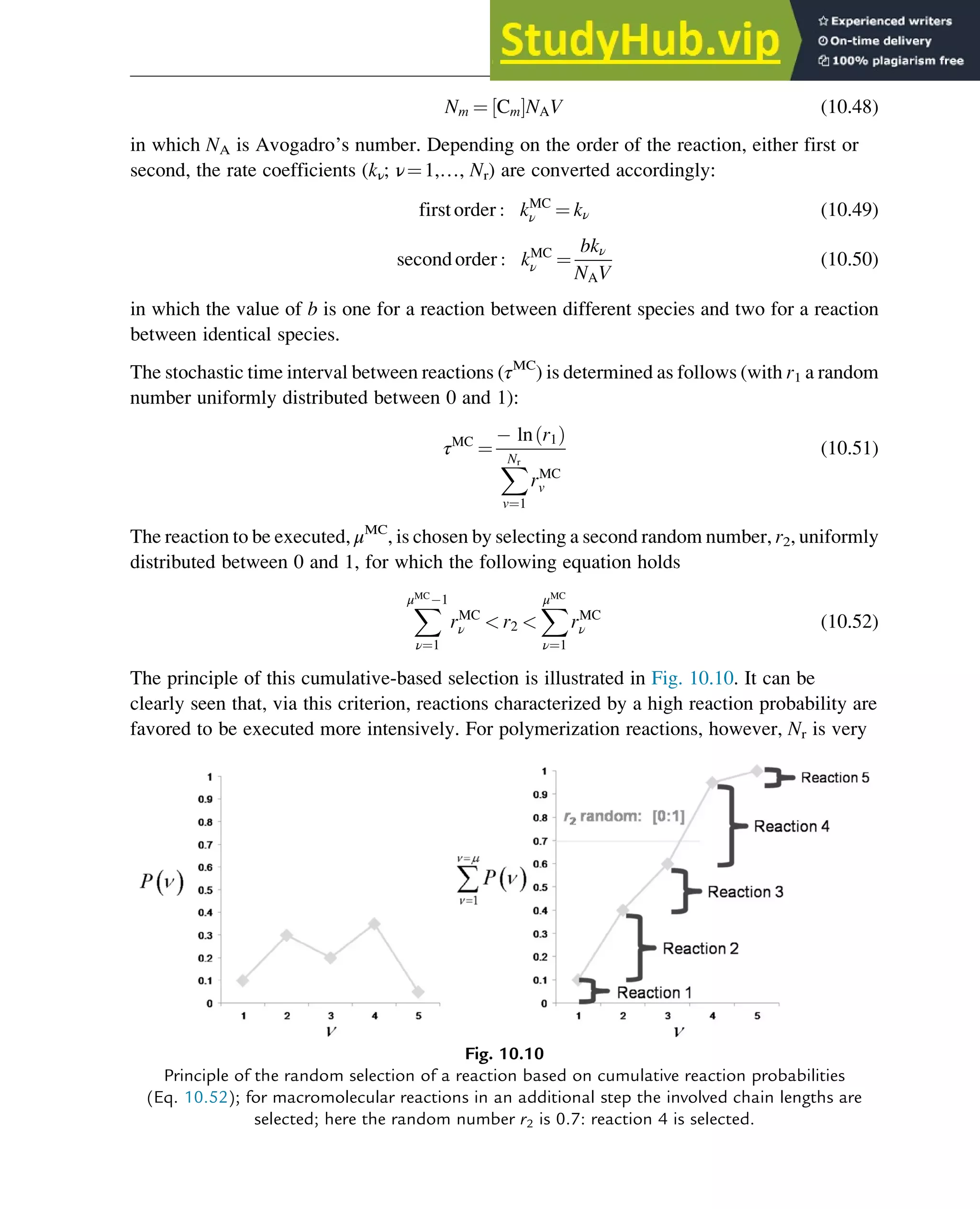
10.2.2 Stochastic Modeling Techniques
In contrast to deterministic modeling techniques, stochastic modeling techniques do not
require the numerical integration of a set of coupled differential equations to simulate chemical
kinetics but only require stochastic executions of discrete events. Two important stochastic
techniques are the Gillespie-based kinetic Monte Carlo (kMC) and the Tobita-based Monte
Carlo technique, which are both addressed in this section. In general, full CLDs are directly
obtained with stochastic modeling approaches as long as a sufficiently high resolution, that is, a
sufficiently large initial number of molecules, is selected.
10.2.2.1 Gillespie-based kMC technique
The most frequently applied kMC algorithm to study polymerization processes is that developed
by Gillespie (1977). In this algorithm, different species are tracked in a representative
microscopic-scale homogeneousvolume V (eg, 10 20
m3
) and reactions are selected ina discrete
manner via stochastic time steps. For each reaction (ν¼1,…, Nr with Nr the total number of
reactions), a Monte Carlo (MC) reaction probability Pν
MC
is first defined:
Pv
MC
¼
rMC
ν
X
Nr
ν¼1
rMC
ν
(10.47)
in which rν
MC
is the “MC rate of reaction ν” expressed per second.
As in the kMC technique the reactions are represented discretely the reaction rates must thus
be converted from macroscopic values, which are in general on a per volume basis, to stochastic
rates on the basis of the total number of molecules within the scaled reaction volume. In order to
do so, the macroscopic concentrations ([Cm]; m¼1,…, Nsp; with Nsp the number of different
types of species) must be converted into a total number of molecules Nm within V:
322 Chapter 10](https://image.slidesharecdn.com/advanceddataanalysisandmodellinginchemicalengineering-230807160524-2b99ba17/75/Advanced-Data-Analysis-and-Modelling-in-Chemical-Engineering-pdf-325-2048.jpg)
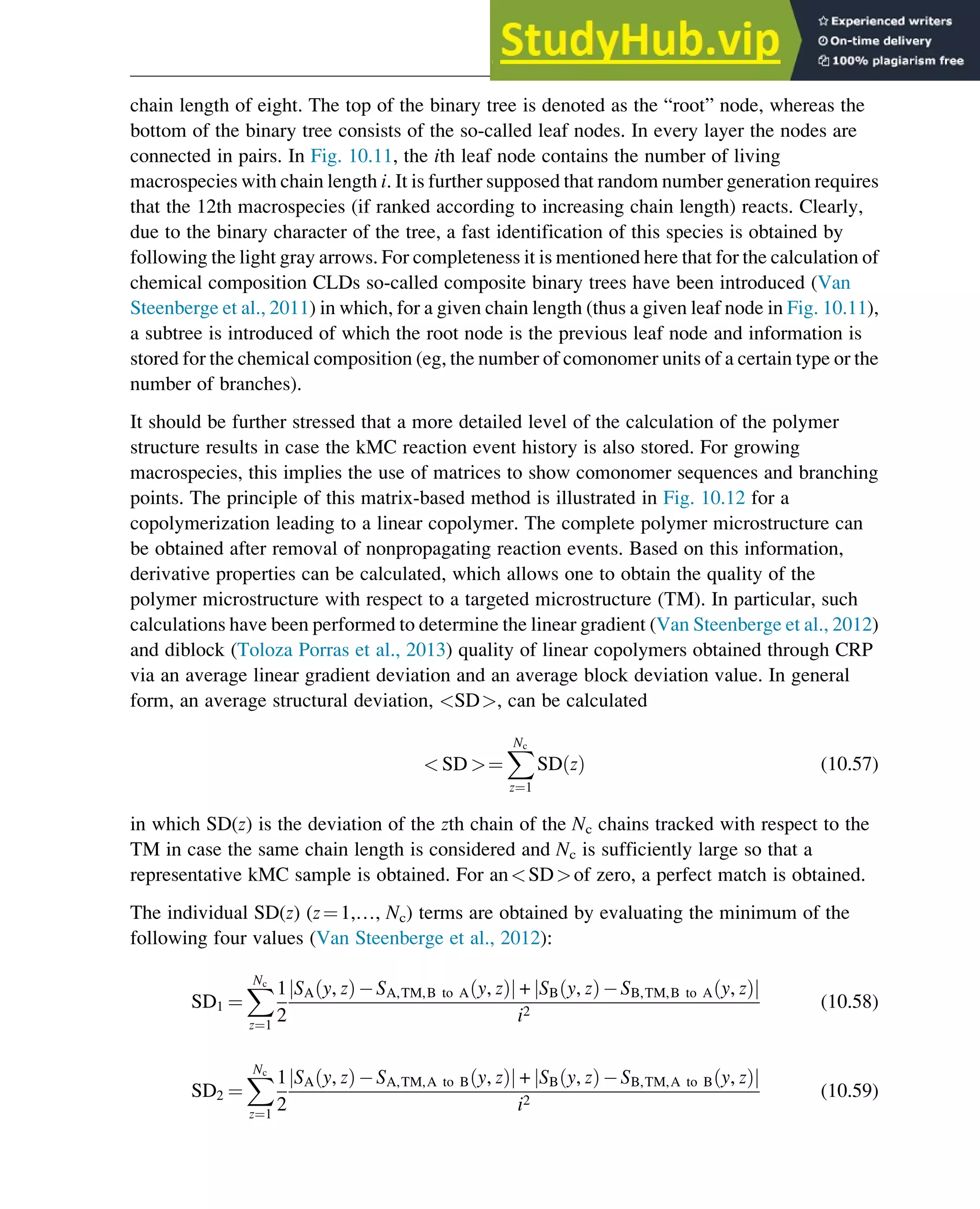
![and Sx
0
(y,z) and S0
x,TM,r(y,z) are the corresponding cumulative functions when counting
from right to left. Four evaluations are needed to treat both monomer types on the same basis
and to account for the possibility that the chains are not ordered a priori.
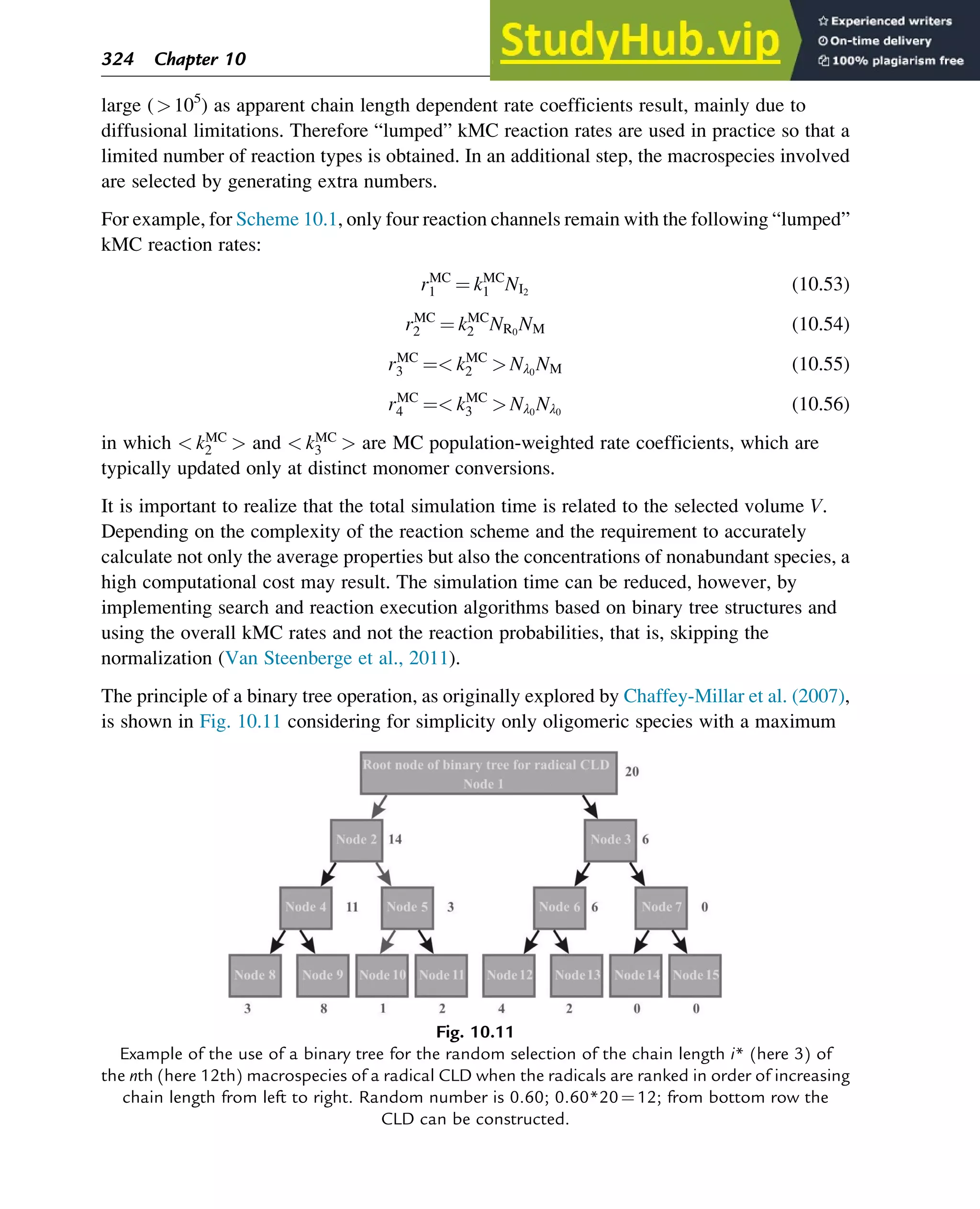
10.2.2.2 Tobita-based MC technique
For branched polymers, the matrix-based kMC approach discussed previously can be extended
by adding additional rows for the composition of the individual branches and storing the
connection points. However, for highly branched polymers this requires very high storage
capacities and intensive coding efforts. Alternatively, the Tobita-based MC technique (Meyer
and Keurentjes, 2005; Tobita, 1993) can be applied to assess the topology of the polymer.
With this technique, the polymer topology is reconstructed a posteriori from building blocks
that are generated via different random numbers. In this section, the basic steps of the
calculation are discussed. This technique is reliable, however, only in case apparent kinetics are
of minor importance.
In a first step, the so-called birth conversion x* is sampled at which an initial zeroth-order
building block (label 0) is generated taking into account the maximum conversion, xmax,
reached. In a second step, the chain length i* of this block is obtained by random selection,
typically following the Flory mass CLD (Tobita, 1993):
mi ¼
i
xn
exp
i
xn
(10.62)
in which mi is the mass fraction of polymer chains with chain length i. The average chain
length xn is determined via the ratio of the reaction rates leading to chain growth and those
leading to termination. The concentrations involved are assessed based on the conversion
selected (eg, via moment equations or pseudoanalytical expressions).
In a third step, for the selected building block, the number of branching points (Nbr) is
determined via sampling based on a binominal distribution (Meyer and Keurentjes, 2005):
p Nbr
ð Þ ¼
i
Nbr
ρNbr
br ρi Nbr
br (10.63)
in which ρbr is a predefined branching probability. Assuming chain transfer to polymer as the
dominant branching point creator, the following expression has been proposed for ρbr:
ρbr ¼
ktp
kp
ln
1 x*
1 i
(10.64)
in which ktp and kp are the transfer to polymer and propagation rate coefficients.
In a fourth step, the birth conversions as well as the lengths have to be selected for these
branches. To obey physical boundaries, the conversion interval [x*, xmax] has to be considered
Polymers: Design and Production 327](https://image.slidesharecdn.com/advanceddataanalysisandmodellinginchemicalengineering-230807160524-2b99ba17/75/Advanced-Data-Analysis-and-Modelling-in-Chemical-Engineering-pdf-330-2048.jpg)
![An important first “compartment model” is based on the division of each compartment into
a discrete number of perfectly mixed segments. For example, in Fig. 10.13, for each
compartment of an industrial-scale reactor for a polymerization process still in nondispersed
medium, two small perfectly mixed segments and one large perfectly mixed segment are
considered. The small segments reflect imperfect mixing (eg, of the initiator) and temperature
gradients (eg, hot spots) at the inlet, whereas the large segment reflects the bulk zone of the
compartment with an internal recycle to both small segments.
Denoting the volume of the kth segment as Vi,k, qVi,k as its exit volumetric flow rate, RMi,k as
the corresponding net monomer production rate, [M]i,k as the monomer concentration, fl as
the lth recycle rate from the third segment, and qV0 as the volumetric feed flow rate with
monomer concentration [M]0, the following continuity equations can be written down for
the monomer in each segment k of a compartment i:
Vi,1
d M
½ Ši,1
dt
¼ M
½ Š0qV0 + M
½ Ši 1,3qVi 1,3 + f1 M
½ Ši,3qVi,3 + RMi,1Vi,1 M
½ Ši,1qVi,1 (10.67)
Vi,2
d M
½ Ši,2
dt
¼ M
½ Ši,1qVi,1 + f2 M
½ Ši,3qVi,3 + RMi,2Vi,2 M
½ Ši,2qVi,2 (10.68)
Vi,3
d M
½ Ši,3
dt
¼ M
½ Ši,2qVi,2 + RMi,3Vi,3 f1 M
½ Ši,3qVi,3 f2 M
½ Ši,3qVi,3 (10.69)
in which it is assumed that the volumetric flow rates are balanced:
qVi,1 ¼ qV0 + qVi 1,3 + f1qVi,3 (10.70)
qVi,2 ¼ qVi,1 + f2qVi,3 (10.71)
1 + f1 + f2
ð ÞqVi,3 ¼ qVi,2 (10.72)
Fig. 10.13
Example of a compartment model with three perfectly mixed segments (two small and one large)
to account for macromixing; Vi,k, volume of segment k in compartment i; qVi,k, exit volumetric flow
rate for segment k in compartment i; qV0, volumetric feed flow rate; fl, recycle ratio (l¼1,2); subscript
V in the flow rates is not shown in order not to overload the figure.
Polymers: Design and Production 329](https://image.slidesharecdn.com/advanceddataanalysisandmodellinginchemicalengineering-230807160524-2b99ba17/75/Advanced-Data-Analysis-and-Modelling-in-Chemical-Engineering-pdf-332-2048.jpg)
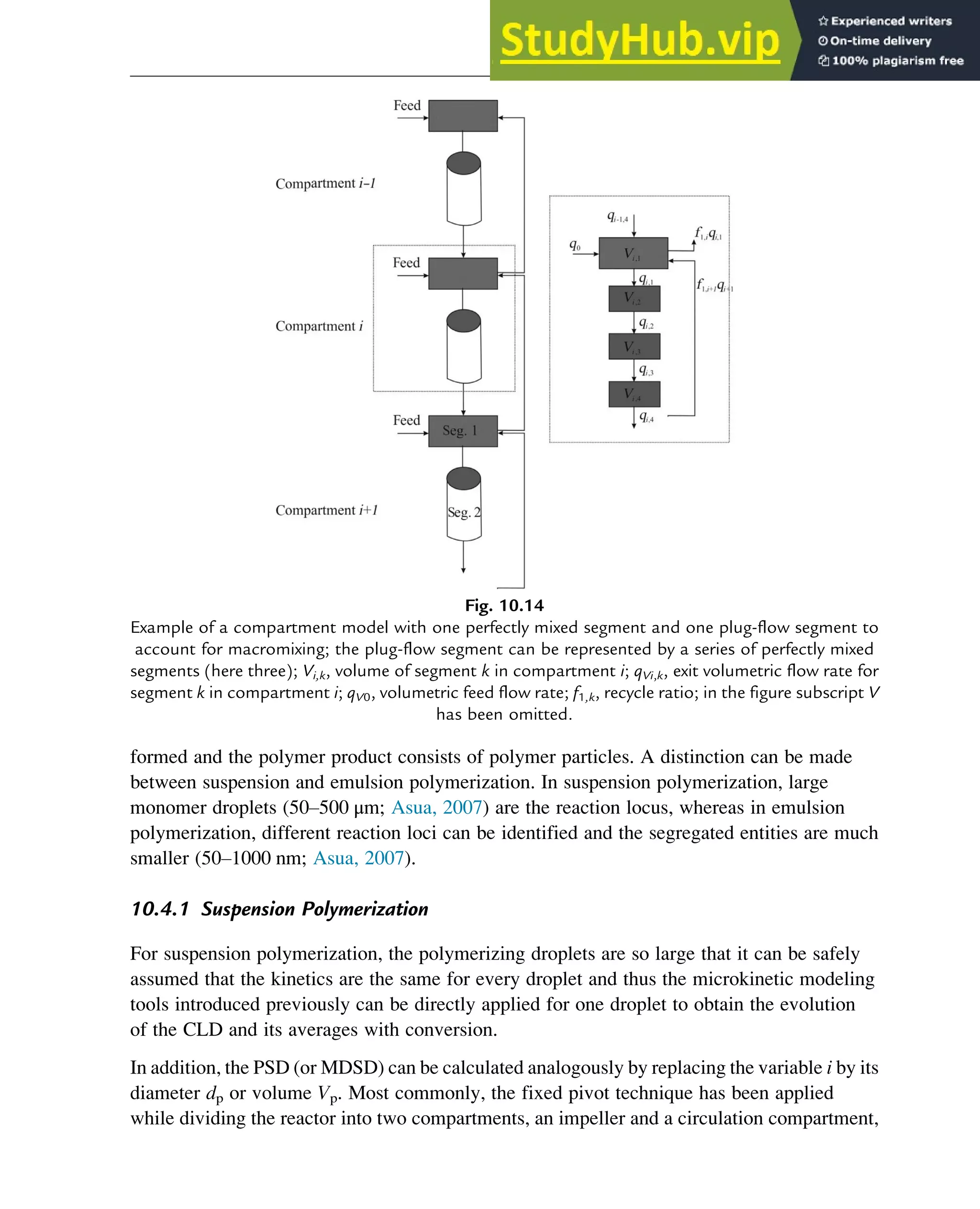
![as shown in Fig. 10.15 (Alexopoulos and Kiparissides, 2005). This distinction is made to
account for the different turbulence intensity in the direct environment of the impeller and the
region away from the impeller, that is, to account for macroscale effects. Such a simplification
is justified, at least as a first approximation, based on CFD simulations of the flow pattern in
batch reactors with an impeller (Alexopoulos et al., 2002).
For each compartment, a population balance is derived as basis for the further
discretization according to the selected pivot elements along the Vp axis and using number
density functions nimp(V,t) and ncirc(V,t) for the impeller and circulation compartments.
These density functions are defined such that nimp(V,t)dV and ncirc(V,t)dV are the numbers of
droplets per unit volume of the impeller and circulation compartments with a volume in the
interval [V, V+dV].
For the impeller compartment with a volume, Vimp, nimp(V,t) can be obtained based on the
following nonlinear integrodifferential equation:
@nimp V, t
ð Þ
δt
¼
ðVmax
V
β U, V
ð Þu U
ð Þg U
ð Þnimp U, t
ð ÞdU
+
1
2
ðV
0
k V U,U
ð Þnimp V U,t
ð Þnimp U, t
ð ÞdU
nimp V, t
ð Þ
ðVmax
0
k V, U
ð Þnimp U, t
ð ÞdU g V
ð Þnimp V, t
ð Þ
+
qV,e
Vimp
ncirc V, t
ð Þ nimp V, t
ð Þ
¼ PBrhs
imp
(10.76)
The first term of the population balance, PBimp
rhs
, relates to the formation of droplets with a volume
in the interval [V, V+dV] by breakage of droplets with a larger volume (maximally Vmax). In this
term, the mesoscale parameter g(U) is the breakage coefficient for a droplet with a volume U,
u(U) is the number of droplets formed upon breakage of a droplet with a volume U (typically
two), and β(U,V) reflects the probability that a droplet with a volume U breaks into a droplet
with a volume V. The second term represents the formation of droplets in the volume interval [V,
Fig. 10.15
Compartment model to calculate the evolution of the monomer droplet size distribution (MDSD) in a
suspension polymerization; Vimp/circ, volume of impeller/circulation compartment.
332 Chapter 10](https://image.slidesharecdn.com/advanceddataanalysisandmodellinginchemicalengineering-230807160524-2b99ba17/75/Advanced-Data-Analysis-and-Modelling-in-Chemical-Engineering-pdf-335-2048.jpg)
![V+dV] by coalescence of two smaller droplets, with the mesoscale parameter k(U,V) the
coalescence coefficient of droplets with a volume of U and V. The third and fourth terms represent
the disappearance of droplets by, respectively, coalescence and breakage, while the last term
expresses the exchange of droplets between the two compartments with qV,e as exchange flow
rate. The analogous nonlinear integrodifferential equation for the circulation compartment can
be obtained by interchanging the subscripts “imp” and “circ” in Eq. (10.76). The mesoscale
parameters are typically obtained by correlations that can depend on the microscale properties via
a dependence on, for instance, the monomer conversion (Asua, 2007).
In practice, the continuous nimp(V,t) function is represented via delta functions:
nimp V, t
ð Þ ¼
X
Nmax
k¼1
N*
imp,k t
ð Þδ V xk
ð Þ (10.77)
in which Nimp,k
* is the contribution to the density function for the droplets in the interval k.
Integration per grid interval of Eq. (10.76) gives
ðVi + 1
Vi
@nimp V, t
ð Þ
@t
dV ¼
ðVi + 1
Vi
PBrhs
imp dV (10.78)
For the left-hand side of this equation, it follows that
ðVi + 1
Vi
@nimp V, t
ð Þ
@t
dV ¼
@
@t
ðVi + 1
Vi
XNmax
k¼1
N*
imp,k t
ð Þδ V xk
ð ÞdV
¼
@
@t
X
Nmax
k¼1
ðVi + 1
Vi
N*
imp,k t
ð Þδ V xk
ð ÞdV ¼
d
dt
N*
imp,k t
ð Þ
(10.79)
Similarly, for each coalescence/breakage term of the right-hand side mathematical
manipulations can be performed. For example, for the positive coalescence contribution
we can write
ðVi + 1
Vi
1
2
ðVx
0
k V U,U
ð Þnr V U,t
ð Þnimp U, t
ð ÞdUdV ¼
1
2
ðVi + 1
Vi
argdV (10.80)
while demanding that this contribution can be related to neighboring pivot volumes:
ðVi + 1
Vi
argdV ¼
ðxi
xi 1
b V, xi
ð ÞargdV +
ðxi + 1
xi
a V, xi
ð ÞargdV (10.81)
in which the functions a and b follow again from the reverse lever rule (see also the CLD
part of the fixed pivot technique):
a V, xi
ð Þ ¼
xi + 1 V
xi + 1 xi
(10.82)
Polymers: Design and Production 333](https://image.slidesharecdn.com/advanceddataanalysisandmodellinginchemicalengineering-230807160524-2b99ba17/75/Advanced-Data-Analysis-and-Modelling-in-Chemical-Engineering-pdf-336-2048.jpg)
![n ¼
X1
n¼0
nNp n
ð Þ
X
1
n¼0
Np n
ð Þ
(10.89)
The polymerization rate with respect to the total volume of the reactor Vr is subsequently
given by
rp ¼ k2 M
½ Šp
nNp
NAVr
(10.90)
in which [M]p is the monomer concentration per particle, which is assumed to be known, and k2
is the propagation rate coefficient (Scheme 10.4).
In case it is assumed that radical initiation occurs in the water phase and radicals can only enter
(absorb), exit (desorb), propagate, and terminate by disproportionation (Scheme 10.4), and
chain length dependencies can be neglected, Np(n) can be calculated using the so-called
Smith-Ewart (Smith and Ewart, 1948) equations (n0):
dNp n
ð Þ
dt
¼ 1 δ n
ð Þ
ð Þkentry Rw
½ ŠNp n + 1
ð Þ + kexit n + 1
ð ÞNp n + 1
ð Þ
+
kto
NAVp
n + 2
ð Þ n + 1
ð Þ Np n + 2
ð Þ kentry Rw
½ ŠNp n
ð Þ
kexitnNp n
ð Þ
kto
NAVp
n n 1
ð ÞNp n
ð Þ
(10.91)
d Rw
½ Š
dt
¼ 2kdis I2w
½ Š + kexit
n
Np
NAVw
2ktw Rw
½ Š2
kentry Rw
½ Š
Np
NAVw
(10.92)
d I2w
½ Š
dt
¼ kdis I2w
½ Š (10.93)
where kentry is the entry or absorption coefficient, kexit is the exit or desorption coefficient, kdis is
the dissociation rate coefficient, and kto/w is the termination rate coefficient in the oil/water
phase. Furthermore, Vw is the volume of the water phase, [I2w] is the concentration of
conventional radical initiator I2 in the water phase, and [Rw] is the total concentration of
radicals in the water phase.
Note that in order to solve Eqs. (10.91)–(10.93), the concentrations of nonradical
components in the individual particles do not have to be known. In contrast, for CRP these
concentrations do have to be known and multidimensional Smith-Ewart equations are needed to
accurately describe the polymerization kinetics. Based on Scheme 10.2 with an oil-soluble
NMP initiator R0X, it follows that if a differentiation is made between the number of NMP
initiator radicals n0, the number of macroradicals n (as before), and the number of nitroxide
Polymers: Design and Production 337](https://image.slidesharecdn.com/advanceddataanalysisandmodellinginchemicalengineering-230807160524-2b99ba17/75/Advanced-Data-Analysis-and-Modelling-in-Chemical-Engineering-pdf-340-2048.jpg)
![κ ¼ Finst
pA 1 Finst
pA
ffiffiffiffiffiffiffiffiffiffiffiffiffiffiffiffiffiffiffiffiffiffiffiffiffiffiffiffiffiffiffiffiffiffiffiffiffiffiffiffiffiffiffiffiffiffiffiffiffiffiffiffiffiffiffiffiffiffiffi
1 4Finst
pA 1 Finst
pA
1 rArB
ð Þ
r
(10.103)
in which FpA
inst
is the instantaneous composition based on the propagation rates using the
comonomer feed concentrations, FpA is the composition of a given polymer chain (in terms of the
mole fraction of A units in the copolymer), and rA and rB are the monomer reactivity ratios:
rA ¼
kpAA
kpAB
(10.104)
rB ¼
kpBB
kpBA
(10.105)
in which kpM1M2
is the propagation rate coefficient for the addition of a living macrospecies
ending in a monomer unit M1 to a monomer of type M2.
The following distribution has been proposed for a single CLD in case long-chain branches can
be formed (Asua, 2007):
m i, zbr
ð Þ ¼
1
2zbr + 1
ð Þ!
i2zbr + 1 1
xn
ð Þ2zbr + 1
exp
i
xn
(10.106)
with zbr the number of long-chain branches considered. For a zbr equal to zero, the Flory
distribution is obtained.
More recently, so-called multigrain models have been developed (Asua, 2007; Tobita and
Yanase, 2007) to describe polymerizations with solid catalysts in a more detailed manner,
including a clear link between the micro- and mesoscale. In such models, the polymer
growth and the possibility to form radial concentration and temperature gradients are accounted
for. The catalyst particle is seen as an agglomeration of macrograins, which in turn are
composed of micrograins, as depicted in Fig. 10.17. The catalyst sites are assumed to be present
at the surface of the catalyst particle.
First, the monomer concentration profile in the macrograin (Ma[rmac,t]) can be calculated based on
εp
@ Mmac
½ Š
@t
¼
1
r2
mac
@
@rmac
Deff,Mr2
mac
@ Mmac
½ Š
@rmac
RM,mic (10.107)
in which the particles are assumed to be spherical, εp is the porosity, rmac is the radial position with
respect to the center of the macrograin, RM,mic is the monomer disappearance rate toward the
micrograins, and Deff,M is the effective monomer diffusion coefficient, as defined by
Deff,M ¼
Db,Mεp
τp
(10.108)
in which Db,M is the bulk monomer diffusivity and τp is the tortuosity of the catalyst particle.
340 Chapter 10](https://image.slidesharecdn.com/advanceddataanalysisandmodellinginchemicalengineering-230807160524-2b99ba17/75/Advanced-Data-Analysis-and-Modelling-in-Chemical-Engineering-pdf-343-2048.jpg)
![As initial condition, it is typically assumed that the concentration profile is constant:
Mmac
½ Š rmac, 0
ð Þ ¼ Mmac
½ Š0 (10.109)
Furthermore, the following boundary conditions can be used:
@ Mmac
½ Š
@rmac
0, t
ð Þ ¼ 0 (10.110)
Deff,M
@ Mmac
½ Š
@rmac
Rmac, t
ð Þ ¼ ktf Mb
½ Š Mmac
½ Š
ð Þ (10.111)
in which Rmac is the radius of the macrograin, ktf is a mass transfer coefficient, and [Mb] is the
bulk monomer concentration.
For the micrograins, the analogous equation is
@ Mmic
½ Š
@t
¼
1
r2
mic
@
@rmic
Dp,Mr2
mic
@ Mmic
½ Š
@rmic
(10.112)
in which rmic is the radial position with respect to the microparticle center, Dp,M is the
diffusivity of the monomer in the polymer layer around the microparticle of radius Rmic and
original size Rc (surface location). Dp,M is given by the ratio of the diffusivity of the monomer in
the amorphous phase and a correction factor for the presence of crystallites. The following
boundary conditions are used:
Mmic
½ Š Rmic, t
ð Þ ¼ Meq
(10.113)
4πR2
cDp,M
@ Mmic
½ Š
@rmic
Rc, t
ð Þ ¼
4
3
πR3
cRV
M,mic (10.114)
Fig. 10.17
Principle of a multigrain model for the description of radial temperature and concentration gradients
in heterogeneous polymerizations with solid catalysts. A macrograin (radius Rmac) consists of
micrograins (radius Rmic with polymer layer, Rc without polymer layer) in concentric layers surrounded
by the gas phase.
Polymers: Design and Production 341](https://image.slidesharecdn.com/advanceddataanalysisandmodellinginchemicalengineering-230807160524-2b99ba17/75/Advanced-Data-Analysis-and-Modelling-in-Chemical-Engineering-pdf-344-2048.jpg)
![in which RM,mic
V
is the monomer consumption rate per unit volume of micrograin particle, which
is linked to the microkinetics, and [Mmic]eq is the equilibrium concentration, which can be
linked to the macrograin concentration through a partition coefficient. As initial condition,
again a constant profile is typically selected:
Mmic
½ Š rmic, 0
ð Þ ¼ Mmic
½ Š0 (10.115)
For the temperature profile, analogous equations can be derived (Asua, 2007; Tobita and
Yanase, 2007).
10.6 Conclusions
Several numerical tools have been developed and successfully applied to model the polymer
microstructure as a function of monomer conversion and process conditions. In this chapter,
these tools have been reviewed and applied to model the polymer microstructure for both
radical and catalytic chain-growth polymerizations, which are mechanistically the most
important polymerization processes. Attention is focused both on the accurate simulation of the
CLD and the PSD, following a multiscale modeling approach. The numerical tools
discussed can be applied also for step-growth polymerizations provided that the model
parameters are available or can be determined experimentally.
A main distinction has been made between deterministic and stochastic modeling techniques.
A further distinction has been proposed based on the scale for which the mathematical
model must be derived (eg, micro-, meso-, and/or macroscale). Notably, the complexity of the
model approach depends on the desired model output. Detailed microstructural information
is only accessible using advanced modeling tools but these are associated with an increase high
in computational cost. The advanced models allow one to directly relate macroscopic
properties to the polymer synthesis procedure and, thus, to broaden the application market
for polymer products, based on a fundamental understanding of the polymerization kinetics
and their link with polymer processing.
Nomenclature
A, B comonomer type
Apivot function predefined by Eq. (10.38)
arg short notation for part of population balance to obtain nimp/circ(V,t)
ak kth expansion coefficient for Galerkin formulation
B0
representative matrix for polymerization kinetics
cp specific heat capacity at constant pressure (J kg 1
K 1
)
Db,M bulk monomer diffusivity (m2
s 1
)
Deff,M effective monomer diffusion coefficient (m2
s 1
)
Dp,M diffusivity of the monomer in the polymer layer (m2
s 1
)
342 Chapter 10](https://image.slidesharecdn.com/advanceddataanalysisandmodellinginchemicalengineering-230807160524-2b99ba17/75/Advanced-Data-Analysis-and-Modelling-in-Chemical-Engineering-pdf-345-2048.jpg)
![Sx,TM,r(y,z) cumulative number of monomer units of type x at position y of the targeted chain
in the direction r (always defined from “left to right”) with the same length as the
considered chain z as counted from “left to right”
Sx
0
(y,z) cumulative number of monomer units of type x at position y in chain z (chain
length: i) of the kMC sample as counted from “right to left”
S0
x,TM,r(y,z) cumulative number of monomer units of type x at position y of the targeted chain
in the direction r (always defined from “left to right”) with the same length as the
considered chain z as counted from “right to left”
T temperature (K)
U volume of droplet (m3
)
u(U) number of droplets formed upon breakage of a droplet with volume U
V volume (m3
)
Vmax indicates border of size domain for droplets in fixed pivot method (m3
)
Vp particle volume (m3
)
Vr reactor volume (m3
)
X nitroxide
xs sth order average chain length; s¼1, 2, 3 or n, m, z
x* birth conversion (Tobita-based MC)
x** birth conversion of branch (Tobita-based MC)
x*** birth conversion for branch created in an earlier stage
y parameter for Stockmayer distribution
z complex variable (pgf method) or chain number (matrix-based kinetic MC)
zbr number of long-chain branches
[A] concentration of nonmacromolecule A (mol m 3
)
[I2] concentration of radical initiator (mol m 3
)
[M] concentration of monomer (mol m 3
)
[Pi] concentration of dead polymer chain with chain length i (mol m 3
)
[Pk
*] concentration of dead polymer chains in the chain length domain k
(mol m 3
)
[R0] concentration of (NMP) initiator radical (mol m 3
)
[Ri] concentration of living polymer chain with chain length i (mol m 3
)
[RiX] concentration of dormant polymer chain with chain length i (mol m 3
)
[Rk
*] concentration of living polymer chains in the chain length domain k
(mol m 3
)
[Rw] total concentration of radicals in the water phase (mol m 3
)
k,s sth order population-weighted rate coefficient (mol m 3
s 1
)
SD average structural deviation
Greek symbols
β(U,V) probability that a droplet with a volume U breaks into a droplet with a volume V
γ orthogonality factor
Polymers: Design and Production 345](https://image.slidesharecdn.com/advanceddataanalysisandmodellinginchemicalengineering-230807160524-2b99ba17/75/Advanced-Data-Analysis-and-Modelling-in-Chemical-Engineering-pdf-348-2048.jpg)

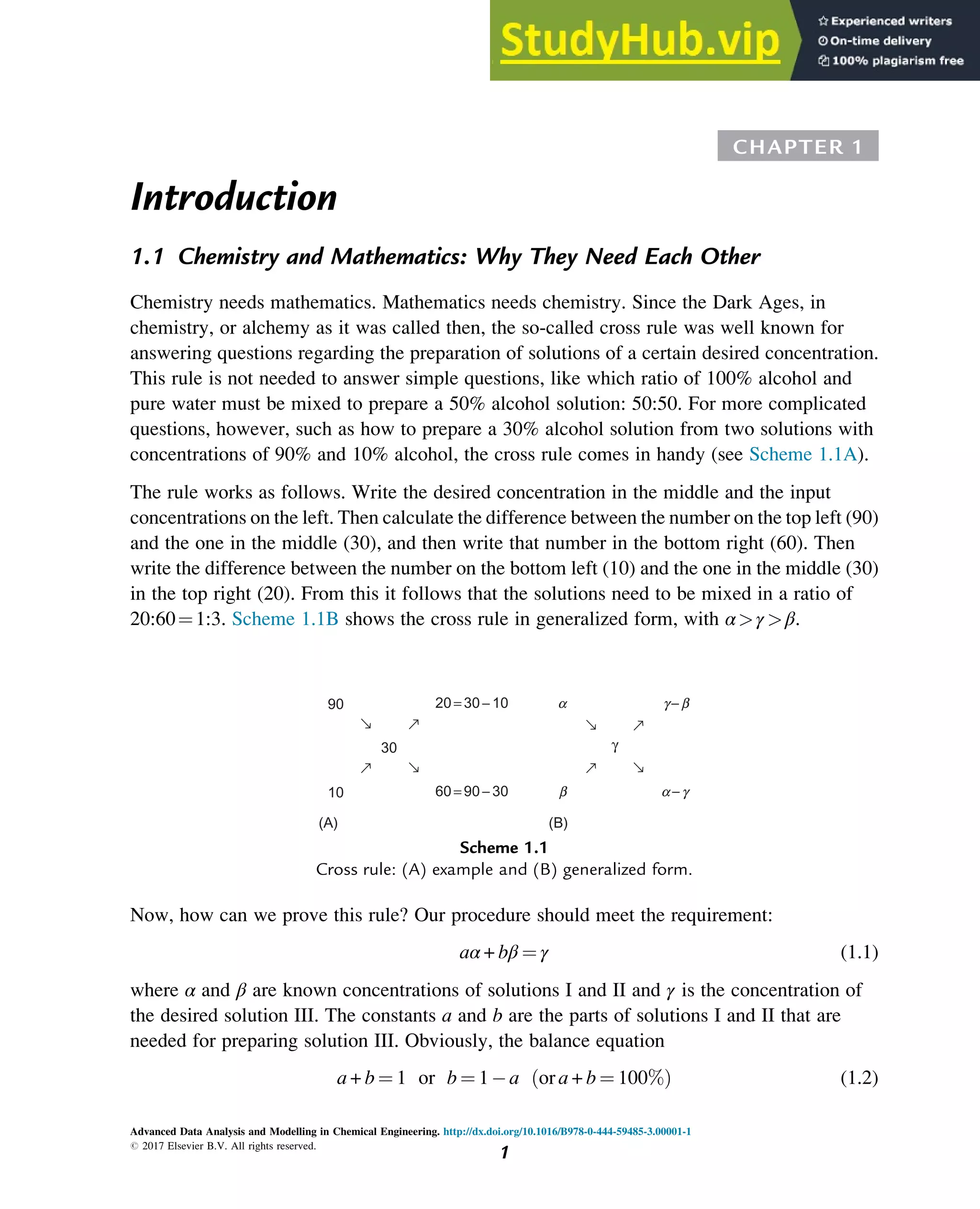
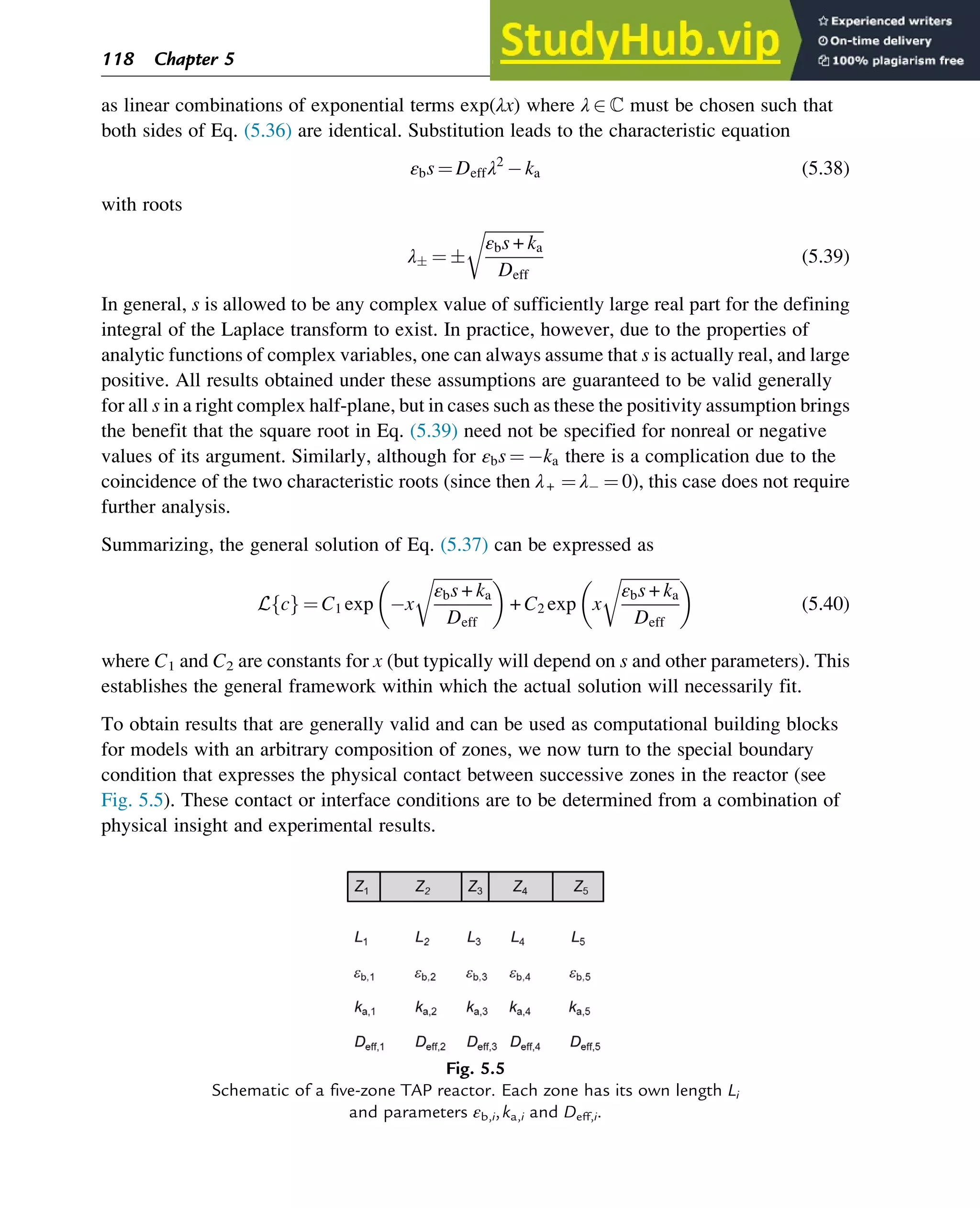
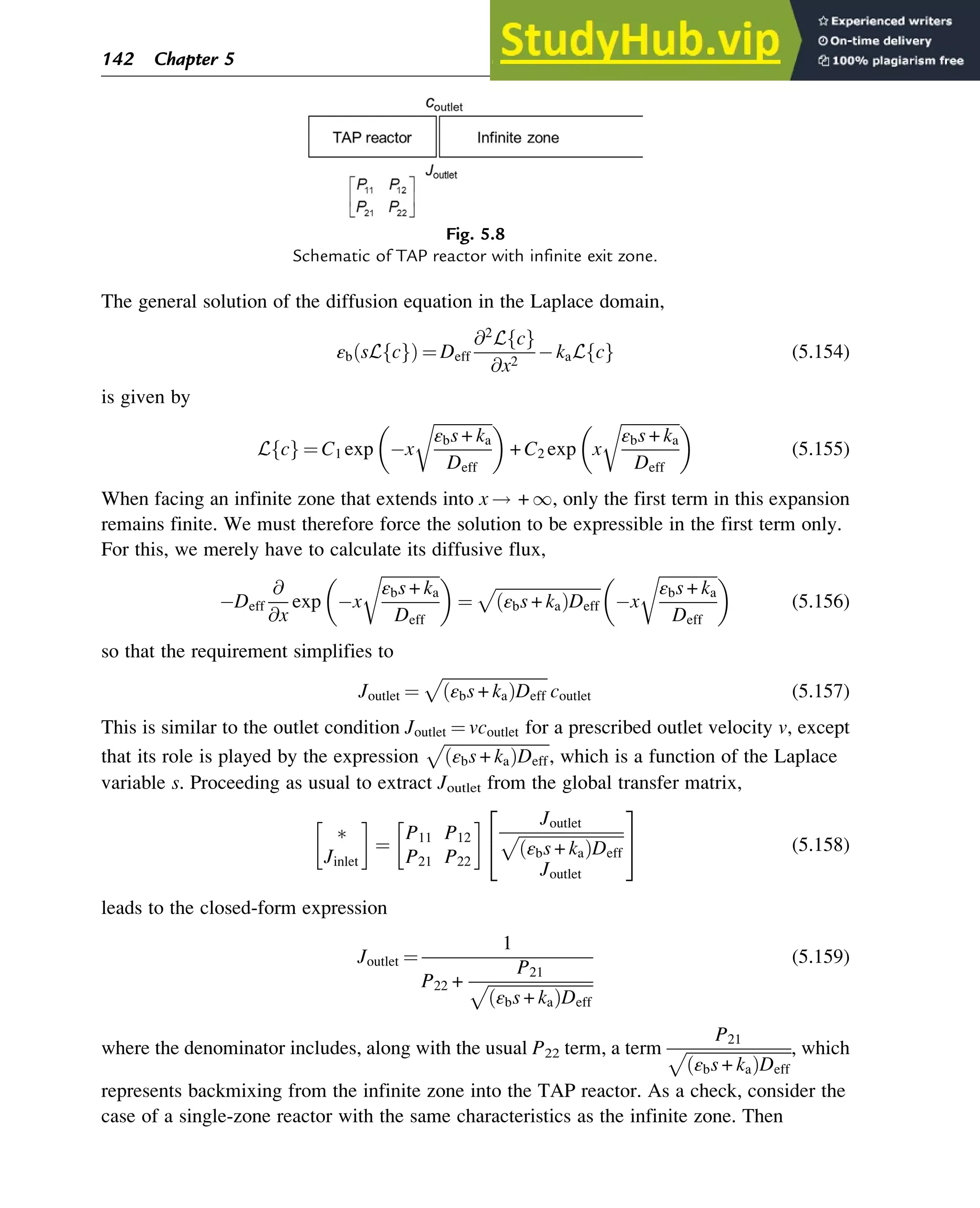
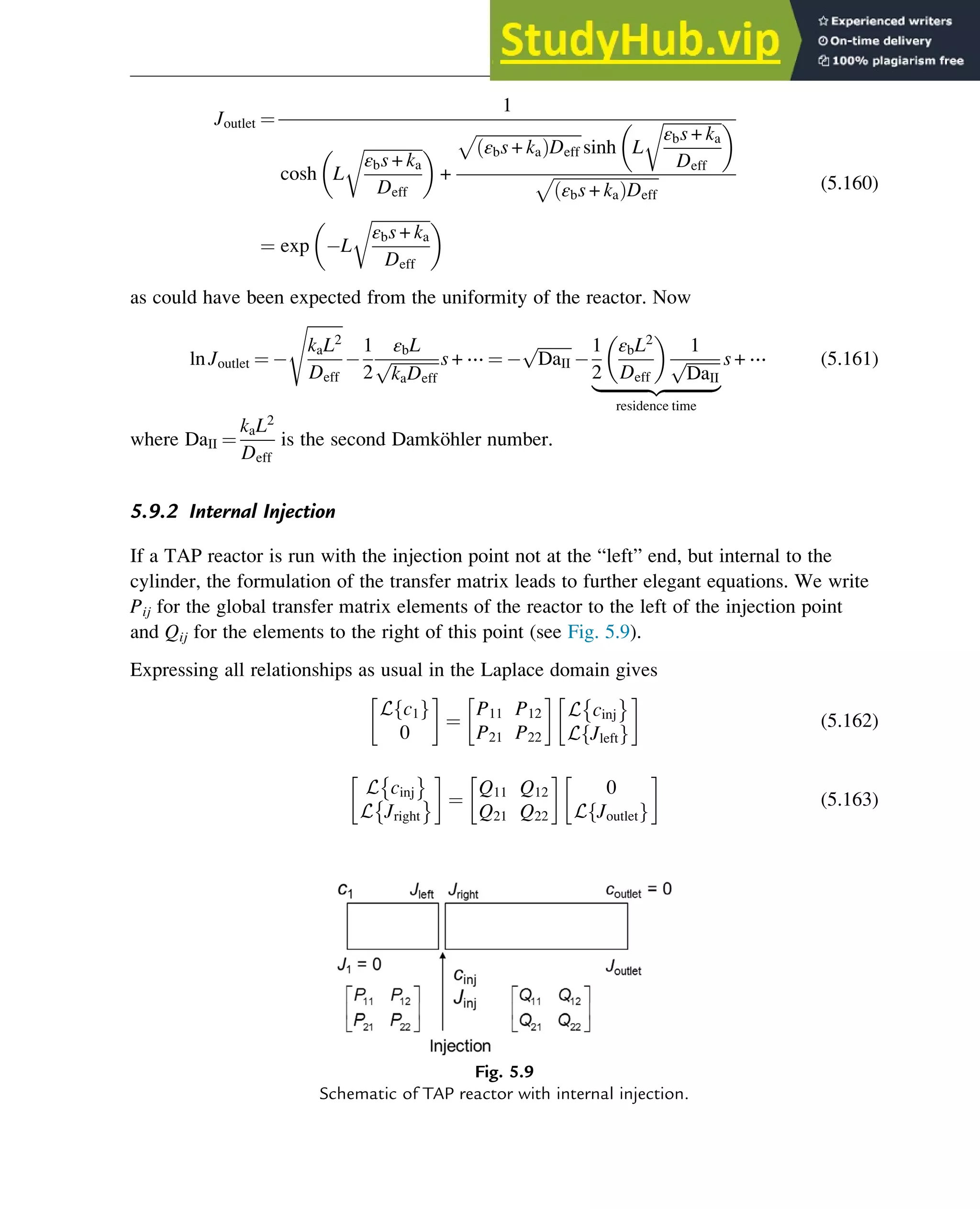
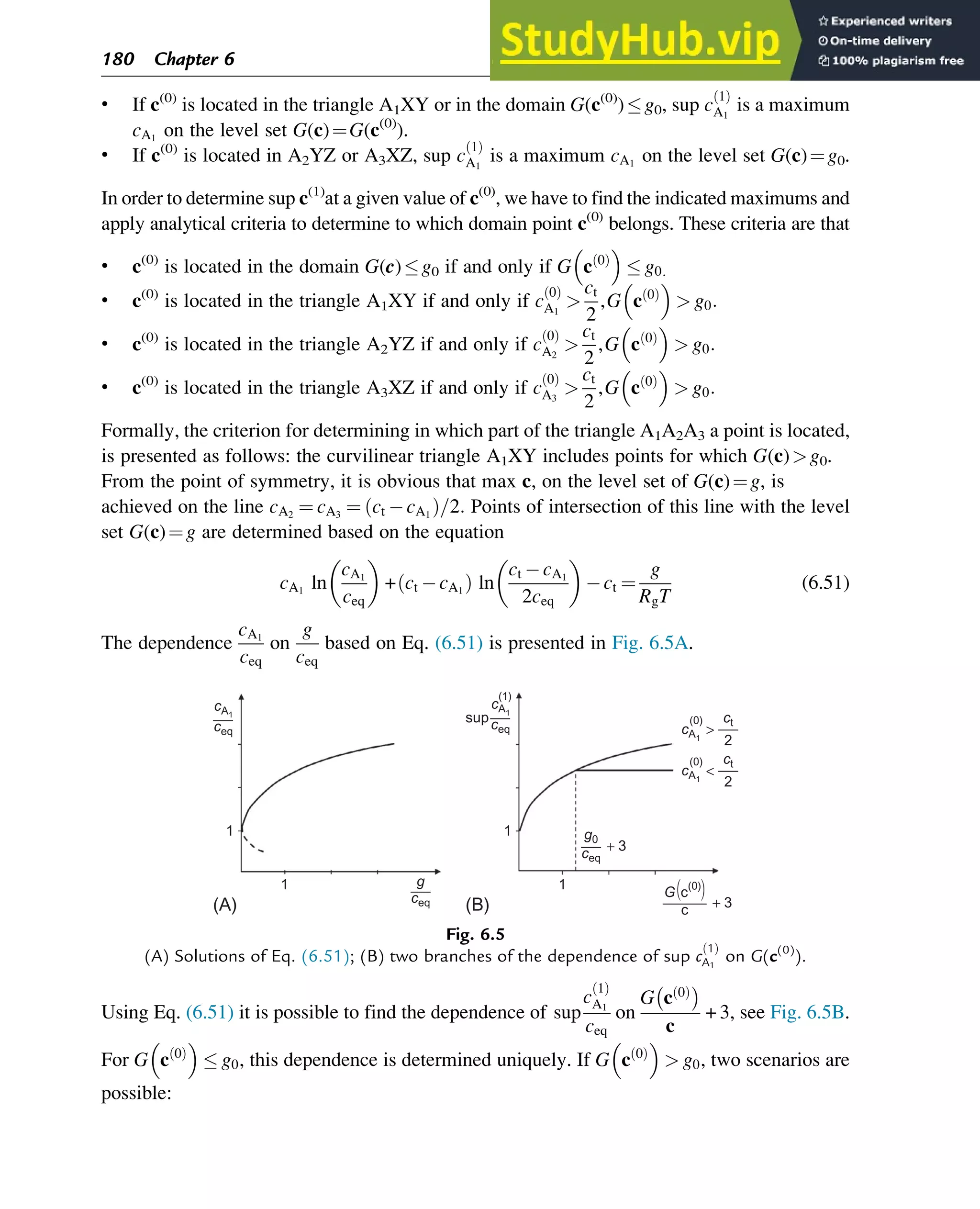
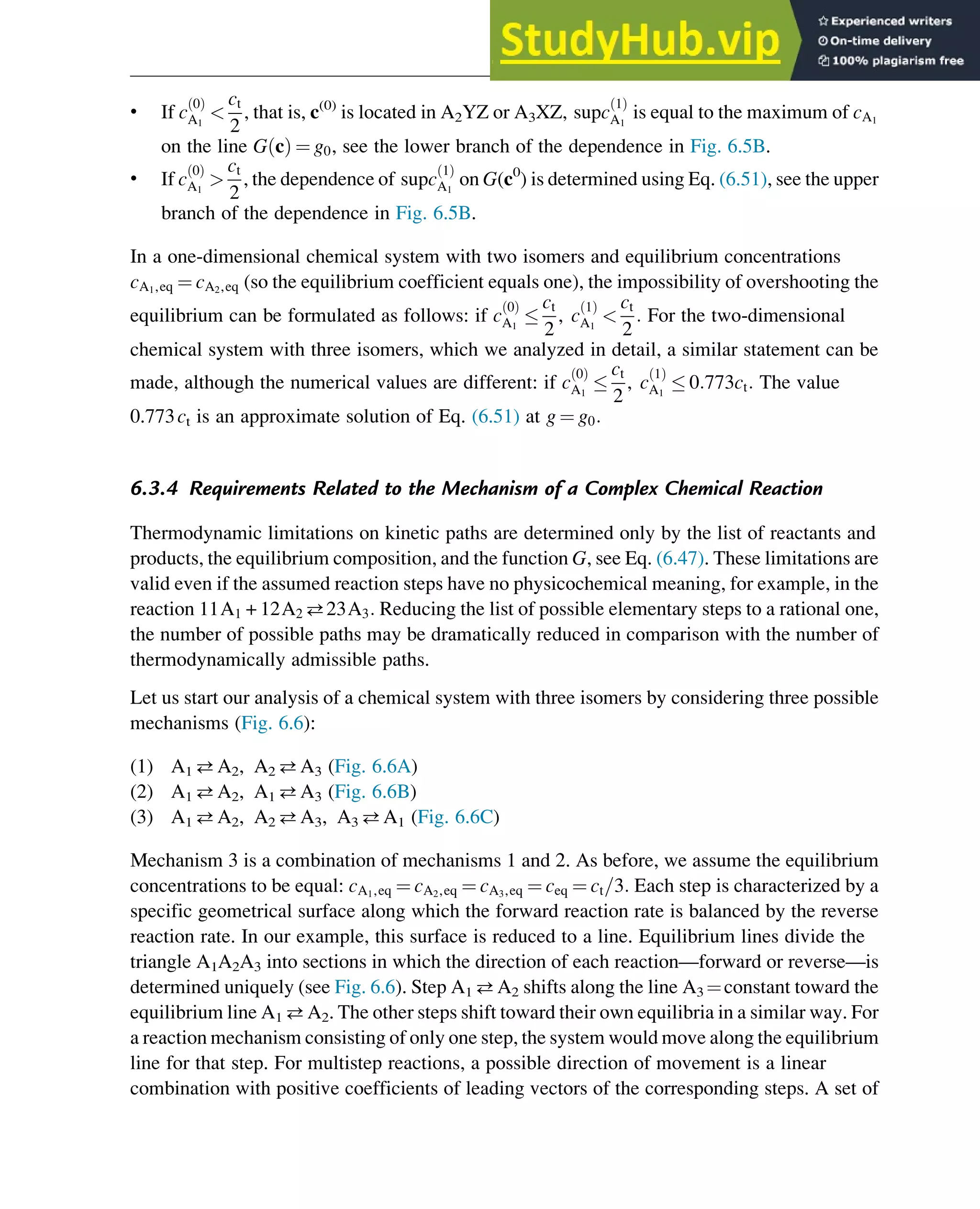
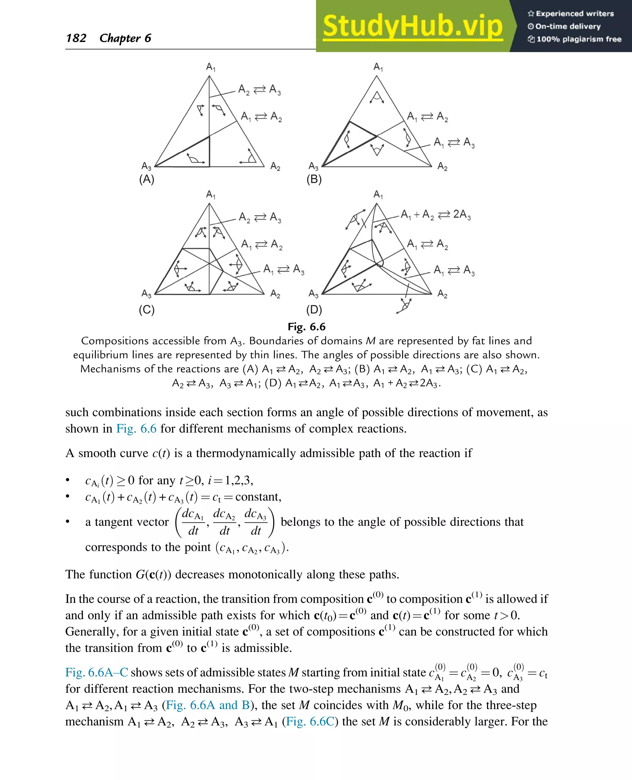
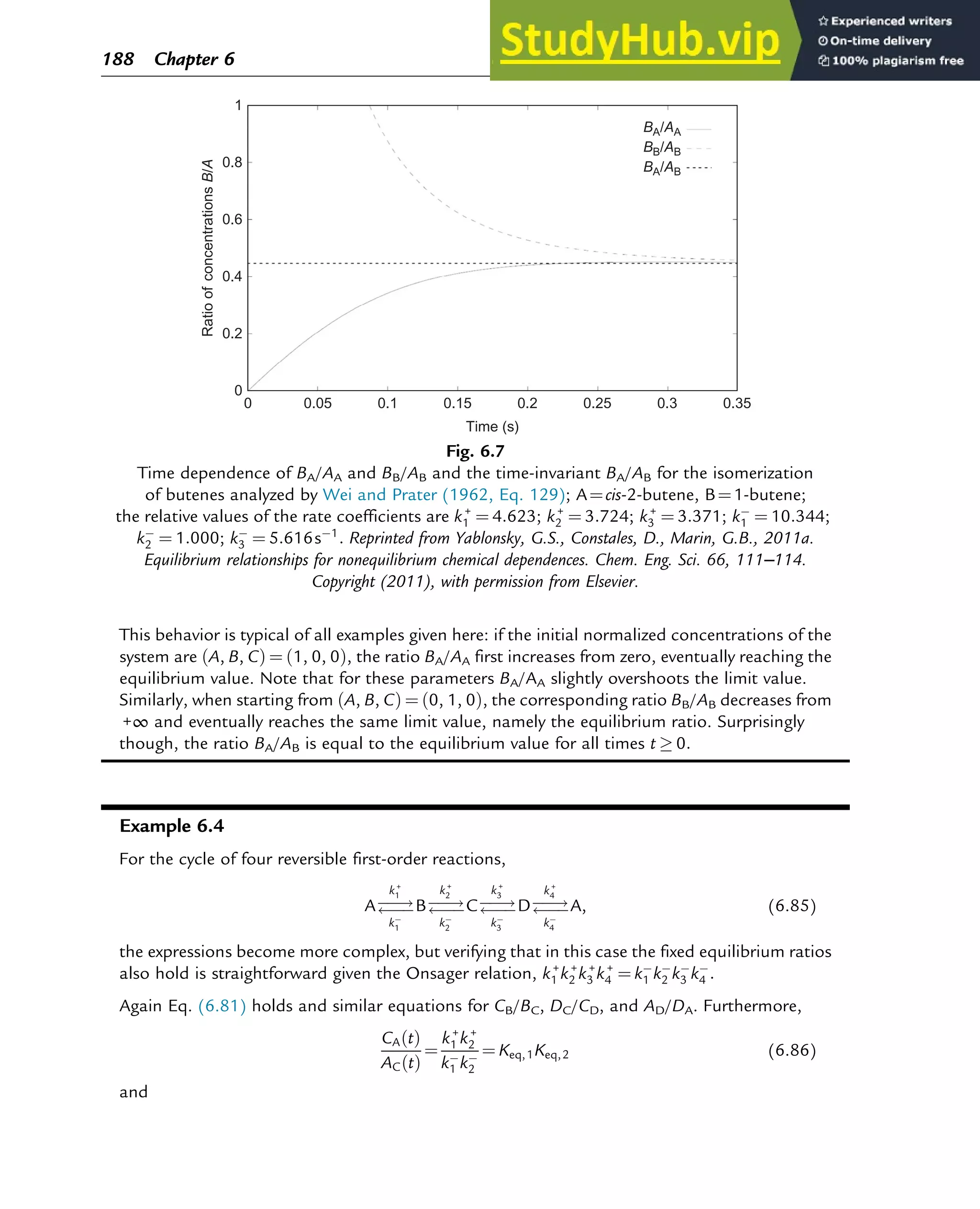
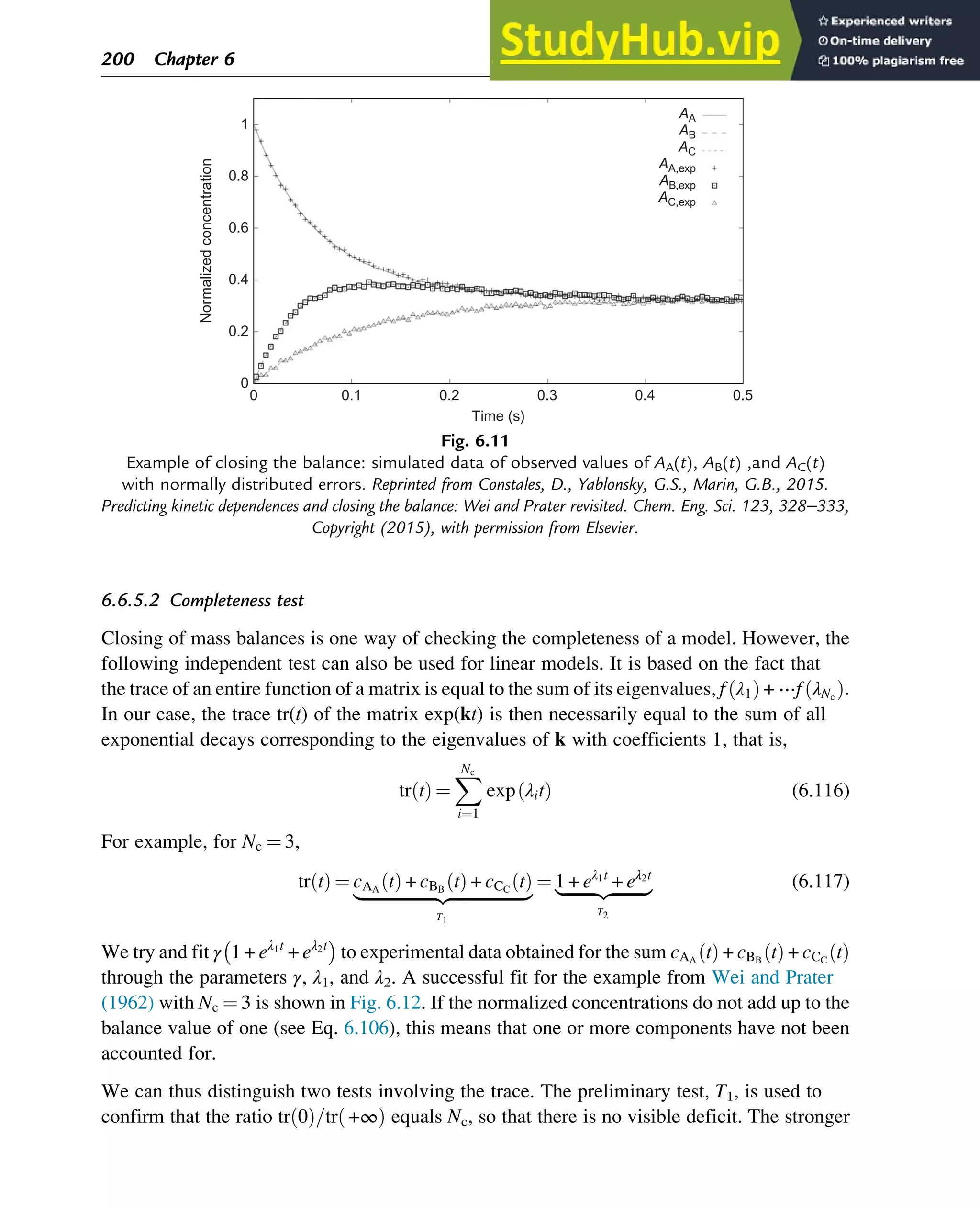
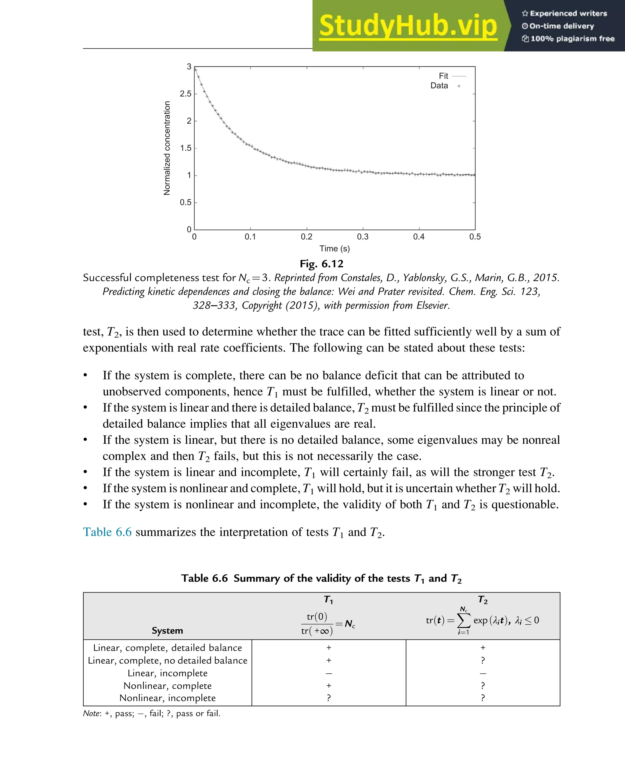
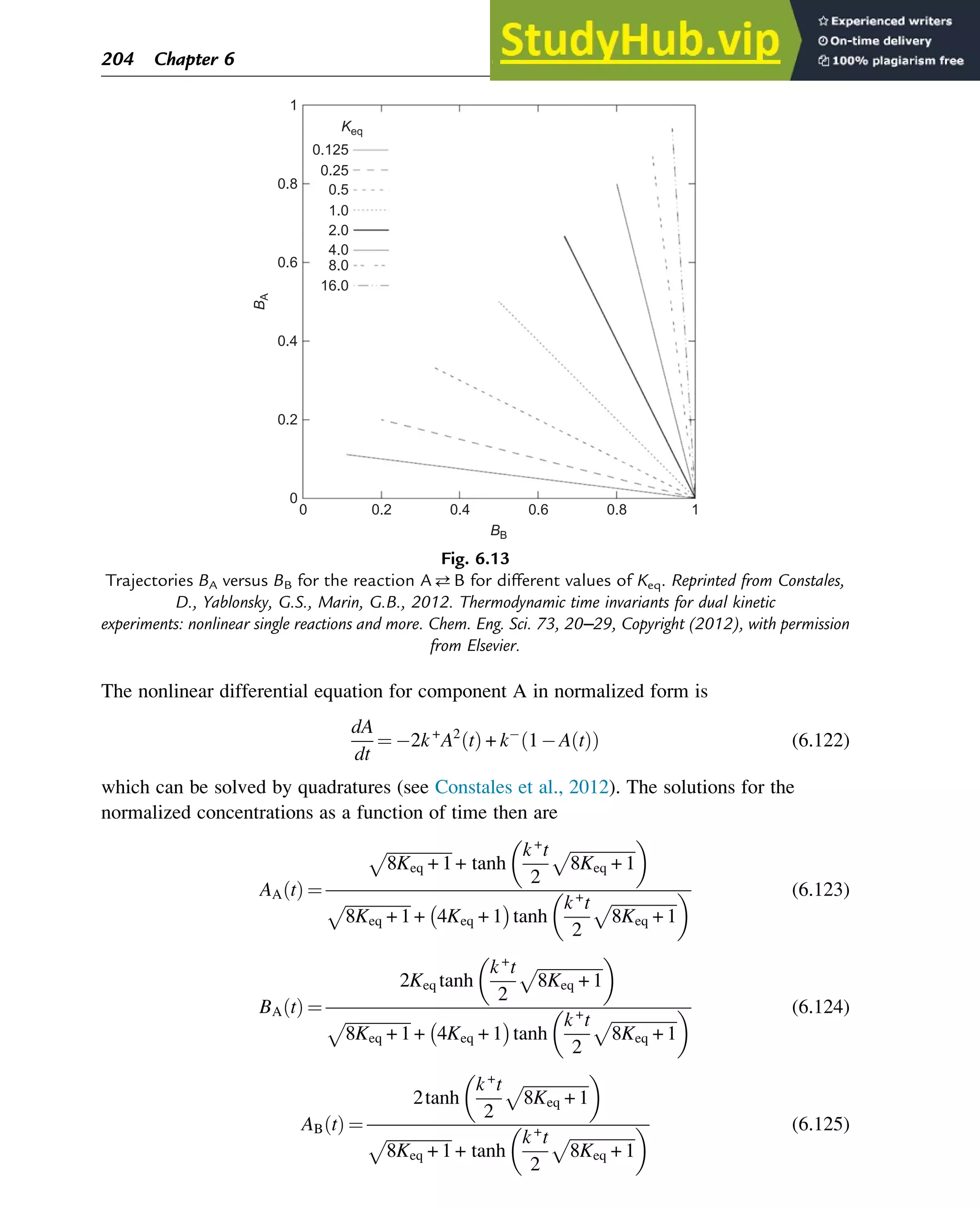
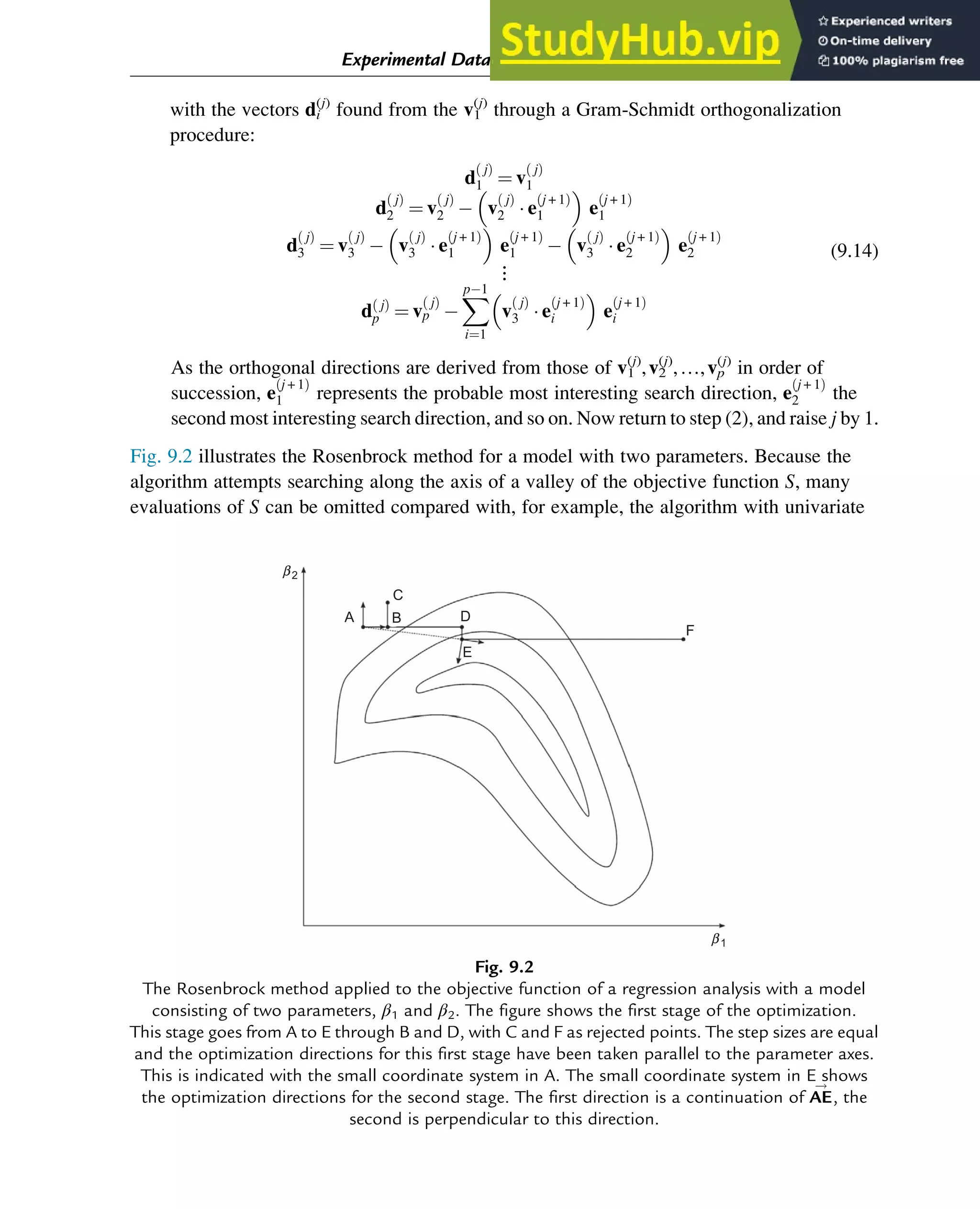
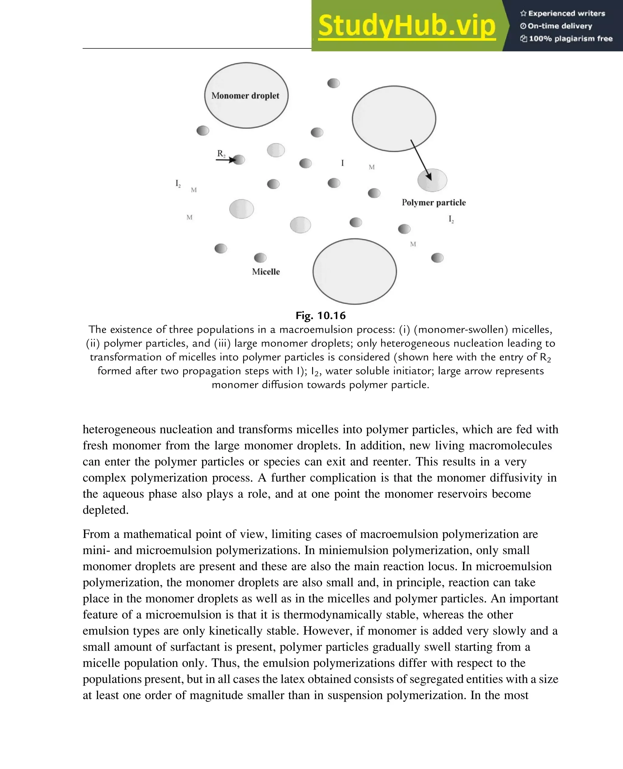
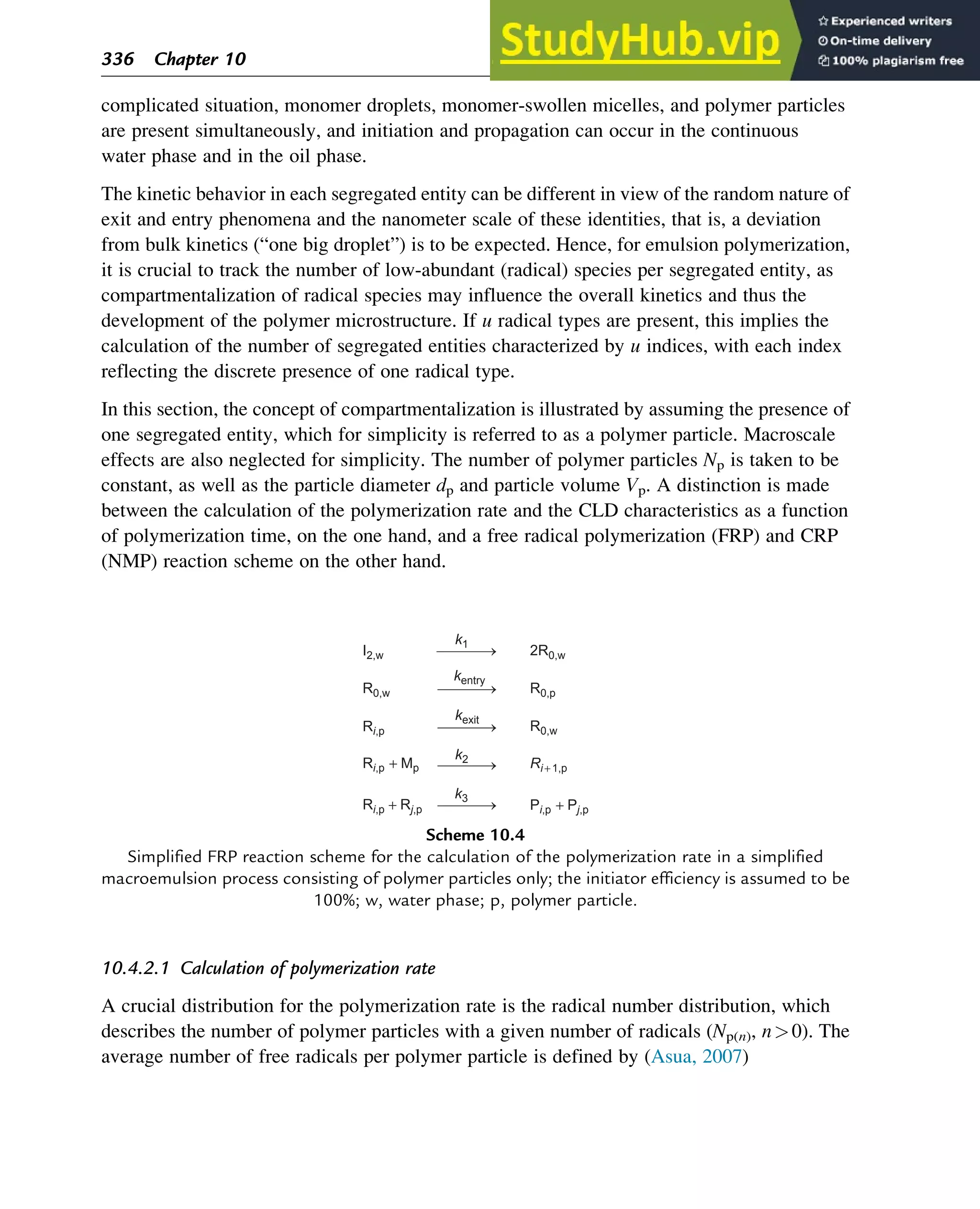
This document provides an introduction to the interrelationship between chemistry and mathematics. It discusses how chemistry relies on mathematics to solve quantitative problems, while mathematics draws inspiration from new chemical phenomena to formulate problems. Historically, concepts in physical chemistry like reaction kinetics led to new mathematical theories. Today, advances in computing enable sophisticated computational modeling across chemical scales. Rigorous theoretical developments in mathematical chemistry have also occurred, especially regarding chemical dynamics and thermodynamics. Overall, the document frames chemistry and mathematics as mutually dependent fields that have influenced each other greatly over time.


