This document compares three methods for obtaining an initial basic feasible solution for transportation problems: Vogel's Approximation Method (VAM), a Proposed Approximation Method (PAM), and a new Minimum Transportation Cost Method (MTCM). It applies all three methods to solve a sample transportation problem with 4 sources and 6 destinations. All three methods produce the same optimal solution and total transportation cost of 450. The document concludes VAM, PAM, and the new MTCM all provide viable options for obtaining the initial basic feasible solution for this transportation problem.

1. Mathematical Theory and Modeling www.iiste.org
ISSN 2224-5804 (Paper) ISSN 2225-0522 (Online)
Vol.4, No.1, 2014
11
A comparative study of initial basic feasible solution methods
for transportation problems
Abdul Sattar Soomro1
Gurudeo Anand Tularam2
Ghulam Murtaa Bhayo3
dr_sattarsoomro@yahoo.co.in, a.tularam@griffith.edu.au, gmsindhi@yahoo.com
1
Professor of Mathematics, Institute of Mathematics and Computer Science, University
of Sindh, Jamshoro, Sindh, Pakistan
2
Senior Lecturer, Mathematics and Statistics, Science Environment Engineering and
Technology [ENV], Griffith University, Brisbane Australia
3
Lecturer, Govt. Degree College, Pano Akil, Sukkur, Sindh, Pakistan
Abstract
In this research three methods have been used to find an initial basic feasible solution for the balanced
transportation model. We have used a new method of Minimum Transportation Cost Method (MTCM) to find
the initial basic feasible solution for the solved problem by Hakim [2]. Hakim used Proposed Approximation
Method (PAM) to find initial basic feasible solution for balanced transportation model and then compared the
results with Vogel’s Approximation Method (VAM) [2]. The results of both methods were noted to be the same
but here we have taken the same transportation model and used MTCM to find its initial basic feasible solution
and compared the result with PAM and VAM. It is noted that the MTCM process provides not only the
minimum transportation cost but also an optimal solution.
Keywords: Transportation problem, Vogel’s Approximation Method (VAM), Maximum
Penalty of largest numbers of each Row
1. Introduction
The transportation problem is a special linear programming problem which arises in many practical applications
in other areas of operation, including, among others, inventory control, employment scheduling, and personnel
assignment [1]. In this problem we determine optimal shipping patterns between origins or sources and
destinations. The transportation problem deals with the distribution of goods from the various points of supply,
such as factories, often known as sources, to a number of points of demand, such as warehouses, often known as
destinations. Each source is able to supply a fixed number of units of the product, usually called the capacity or
availability and each destination has a fixed demand, usually called the requirements. The objective is to
schedule shipments from sources to destinations so that the total transportation cost is a minimum.
There are various types of transportation models and the simplest of them was first presented by Hitchcock
(1941). It was further developed by developed by Koopmans (1949) and Dantzig (1951). Several extensions of
transportation model and methods have been subsequently developed. In general, the Vogel’s approximation
method yields the best starting solution and the north-west corner method yields the worst. However, the latter is
easier, quick and involves the least computations to get the initial solution [5]. Goyal (1984) improved VAM for
the unbalanced transportation problem, while Ramakrishnan (1988) discussed some improvement to Goyal’s
Modified Vogel’s Approximation method for unbalanced transportation problem [6].
Adlakha and Kowalski (2009) suggested a systematic analysis for allocating loads to obtain an alternate optimal
solution [7]. However, the study on alternate optimal solutions is clearly limited in the literature of transportation

2. Mathematical Theory and Modeling www.iiste.org
ISSN 2224-5804 (Paper) ISSN 2225-0522 (Online)
Vol.4, No.1, 2014
12
with the exception of Sudhakar VJ, Arunnsankar N, Karpagam T (2012) who suggested a new approach for
finding an optimal solution for transportation problems [8].
2. Transportation problem and General Computational Procedures
The transportation model of LP can be modeled as follows:
;,0
)(
)(
)cos(
1
1
1 1
jandiallforx
nsdestinatiofromDemandbx
sourcesfromSupplyxtoSubject
ttiontransportaTotalxCZMinimize
ij
m
i
jij
n
j
iij
m
i
n
j
ijij









 
a
where Z : Total transportation cost to be minimized.
Cij : Unit transportation cost of the commodity from each
source i to destination j.
xij : Number of units of commodity sent from source i to destination j.
ia : Level of supply at each source i.
bj : Level of demand at each destination j.
.bDemandSupply
m
1i
i
m
1i
i 











 
a
NOTE: Transportation model is balanced if .bDemandSupply
m
1i
i
m
1i
i 











 
a
Otherwise unbalanced if .b
11












 
m
i
i
m
i
i DemandSupply a
The total number of variables is mn. The total number of constraints is m+n, while the total number of
allocations (m+n–1) should be in feasible solution. Here the letter m denotes the number of rows and n denotes
the number of columns.
Solving Transportation Problems
The basic steps for solving transportation model are:
Step 1 - Determine a starting basic feasible solution. In this paper we use any one method NWCM, LCM, or
VAM, to find initial basic feasible solution.
Step 2 - Optimality condition - If solution is optimal then stop the iterations otherwise go to step 3.
Step 3 - Improve the solution. We use either optimal method: MODI or Stepping Stone method.
Table 1: Transportation array

3. Mathematical Theory and Modeling www.iiste.org
ISSN 2224-5804 (Paper) ISSN 2225-0522 (Online)
Vol.4, No.1, 2014
13
DESTINATIONS
Supply a iD1 D2 …….. ……….. Dn
S1
S2
.
.
.
.
Sm
S
o
u
r
c
e
s
a 1x1n
C1n
……..x12
C12
x11
C11
a 2x2n
C2n
……..
x22
C22
x21
C21
……..……..……..……..……..
a mxmn
Cmn
……..
xm2
Cm2
xm1
Cm1
Balanced model
  

m
1i
n
1j
ji babn……..b2b1
Demand
bj
2. Methodology
The following methods are always used to find initial basic feasible solution for the transportation problems and
are available in almost all text books on Operations Research [5].
The Initial Basic Feasible Solutions Methods are:
(i) Column Minimum Method (CMM)
(ii) Row Minimum Method (RMM)
(iii) North West-Corner Method (NWCM)
(iv) Least Cost Method (LCM)
(v) Vogel’s Approximation Method (VAM)
The Optimal Methods used are:
(i) Modified Distribution (MODI) Method or u-v Method
(ii) Vogel’s Approximation Method (VAM)
3. Initial Basic Feasible Solution Methods and Optimal Methods
There are several initial basic feasible solution methods and optimal methods for solving transportation problems
satisfying supplying and demand.
Initial Basic Feasible Solution Methods
We have used following three methods to find initial basic feasible solution of the balanced transportation
problem:
 Vogel’s Approximation Method (VAM)
 Proposed Approximation method (PAM)
 Minimum Transportation Cost Method (MTCM)
For optimal methods we have used the Modified Distribution (MODI) Method and the Stepping Stone Method
Vogel’s Approximation Method (VAM)

4. Mathematical Theory and Modeling www.iiste.org
ISSN 2224-5804 (Paper) ISSN 2225-0522 (Online)
Vol.4, No.1, 2014
14
This method provides a better starting solution than the North West Corner rule and Least Cost Method. VAM
generally yields an optimum or close to optimum solution.
Algorithm
Step 1. Compute penalty of each row and a column. The penalty will be equal to the difference between the
two smallest shipping costs in the row or column.
Step 2. Identify the row or column with the largest penalty and assign highest possible value to the variable
having smallest shipping cost in that row or column.
Step 3. Cross out the satisfied row or column.
Step 4. Compute new penalties with same procedure until one row or column is left out.
Note: Penalty means the difference between two smallest numbers in a row or a column.
Proposed Approximation Method (PAM)
This method provides a better starting solution than the North West Corner rule and Least Cost Method. The
PAM generally yields optimum solution or close to optimum solution.
Algorithm
Step 1. Identify the boxes having maximum and minimum transportation cost in
each row and write the difference (penalty) along the side of the table against
the corresponding row.
Step 2. Identify the boxes having maximum and minimum transportation cost in
each column and write the difference (penalty) against the corresponding
column.
Step 3. Identify the maximum penalty. If it is along the side of the table, make
maximum allotment to the box having minimum cost of transportation in that
row. If it is below the table, make maximum allotment to the box having
minimum cost of transportation in that column.
Step 4. If the penalties corresponding to two or more rows or columns are equal,
select the box where allocation is maximum.
Step 5. No further consideration is required for the row or column which is satisfied.
If both the row and column are satisfied at a time, delete the two or column is
assigned zero supply (or demand).
Step 6. Calculate fresh penalty cost for the remaining sub-matrix as in step 1 and
allocate following the procedure of previous step. Continue the process until
all rows and columns are satisfied.
Step 7. Compute total transportation cost for the feasible cost for the feasible
allocations using the original balanced transportation cost matrix.
Minimum Transportation Cost Method (MTCM)
This method provides a better starting solution than the North West Corner rule and Least Cost Method. The
MTCM generally yields optimum solution or close to optimum solution.
Algorithm

5. Mathematical Theory and Modeling www.iiste.org
ISSN 2224-5804 (Paper) ISSN 2225-0522 (Online)
Vol.4, No.1, 2014
15
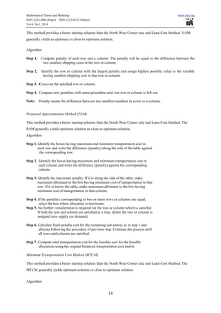
Step 1. Make the table balanced. Compute penalty of each row. The penalty will be equal to the difference
between the two largest shipping costs in the row.
Step 2. Identify the row or column with the maximum penalty and assign possible value to the variable
having smallest shipping cost in that row. If two or more rows corresponding equal penalty then
select the cell with minimum cost of that maximum penalty row.
Step 3. Cross out the satisfied row or column.
Step 4. Write the reduced table and compute new penalties with same procedure until one row or column is left
out. Determine the total minimum cost of occupied cells satisfying m+n-1allocations.
Note: Penalty means the difference between two largest numbers in a row.
Optimal Method
Modified Distribution (MODI) Method
This method always gives the total minimum transportation cost to transport the goods from sources to the
destinations.
Algorithm
1. If the problem is unbalanced, balance it. Setup the transportation tableau
2. Find a basic feasible solution.
3. Set 01 u and determine sui ' and svj ' such that ijji cvu  for all basic variables.
4. If the reduced cost 0 jiij vuc for all non-basic variables (minimization problem), then the
current BFS is optimal. Stop! Else, enter variable with most negative reduced cost and find leaving
variable by looping.
5. Using the new BFS, repeat steps 3 and 4.
4. The Numerical Problem
We have used three methods to find an initial basic feasible solution for the balanced transportation problem [4].
The problem was developed by Hakim [2]. Consider the transportation problem presented in Table 2 - where
there are 4 sources, 6 destinations; the cost is given in the cells, and the supply and demand given in bottom and
right hand end row and column respectively in Table 2.
Table 2: Example problem
Destinations
Sources
1 2 3 4 5 6 Supply
1 1 2 1 4 5 2 30
2 3 3 2 1 4 3 50
3 4 2 5 9 6 2 75
4 3 1 7 3 4 6 20
Demand 20 40 30 10 50 25 175
Solution
Three methods have been used here to find initial basic feasible solution of the above problem and these are
presented in turn.

6. Mathematical Theory and Modeling www.iiste.org
ISSN 2224-5804 (Paper) ISSN 2225-0522 (Online)
Vol.4, No.1, 2014
16
Vogel’s Approximation Method (VAM)
Using VAM the final solution is presented in the Table 3.
Table 3: Solution using VAM
Sources
1 2 3 4 5 6 Supply
1 20 10 30
2 20 10 20 50
3 20 30 25 75
4 20 20
Demand 20 40 30 10 50 25 175
Therefore the total transportation cost determined by the Vogel’s Approximation Method is:
Minimize Z = (20) (1) + (10) (1) + (20) (2) + (10) (1) + (20) (4) +(20) (2) + (30) (6)
+ (25) (2) + (20) (1)
= 20 + 10 + 40 + 10 + 80 + 40 + 180 + 50 + 20
= 450
Solution Proposed Approximation Method (PAM)
The final solution completed using PAM is presented in the Table 4.
Table 4: Solution by PAM
Sources
1 2 3 4 5 6 Supply
1 30 30
2 10 40 50
3 20 20 10 25 75
4 20 20
Demand 20 40 30 10 50 25 175
The total transportation cost by Proposed Approximation Method can be given as:
Minimize Z = (30) (1) + (10) (1) + (40) (4) + (20) (4) + (20) (2) +(10) (6) + (25) (2)
+ (20) (1)
= 30 + 10 + 160 + 80 + 40 + 60 + 50 + 20
= 450
Minimum Transportation Cost Method (MTCM)
The total transportation cost by Minimum Transportation Cost Method is given in Table 5.
Table 5: Solution by MTCM
Sources
1 2 3 4 5 6 Supply
1 20 10 30
2 20 30 50
3 40 10 25 75
4 10 10 20
Demand 20 40 30 10 50 25 175

7. Mathematical Theory and Modeling www.iiste.org
ISSN 2224-5804 (Paper) ISSN 2225-0522 (Online)
Vol.4, No.1, 2014
17
The total transportation Cost by MCTM is given as:
Minimize Z = (20) (1) + (10) (1) + (20) (2) + (30) (4) + (40) (2) +(10) (6) + (25) (2)
+ (10) (3) + (10) (4)
= 20 + 10 + 40 + 120 + 80 + 60 + 50 + 30 +40
= 450
Modified Distribution (MODI) Method
We have found total minimum transportation cost using MODI method by taking initial basic feasible solution
obtained by Minimum Transportation Cost Method (MTCM). The final solution is shown in Table 6.
Table 6: Solution using MODI
Sources
1 2 3 4 5 6 Supply
1 20 10 30
2 20 10 20 50
3 40 10 25 75
4 20 20
Demand 20 40 30 10 50 25 175
The total transportation cost by Modified Distribution Method is given as:
Minimize Z = (20) (1) + (10) (1) + (20) (2) + (10) (1) + (20) (4) + (40) (2) + (10) (6)
+ (25) (2) + (20) (4)
= 20 + 10 + 40 + 10 + 80 + 80 + 60 + 50 +80
= 430
Table 5: A comparison of the methods - VAM, PAM and MTCM and MODI
Initial Basic Feasible
methods
Value of the objective
function
Minimum Value (cost)
VAM 450 Same Result
PAM 450 Same Result
MTCM 450 Same Result
MODI Method 430 Optimal or minimum cost
The cost of transportation shows that the:
(i) Minimum Transportation Cost Method (MTCM), Vogel’s approximation method (VAM), and Proposed
Approximation Method (PAM) provide the same result, not optimal but close to optimal;
(ii) In MTCM, we have used penalty of maximum numbers of each row yet not of each
column;
(iii) In VAM and PAM, the penalty of smallest numbers of each row and column are applied;
(iv) In MTCM, the penalty of each row makes the problem simple, easy and takes a short time in
calculation; and
(v) In VAM and PAM, the penalty of each row and column makes the problem lengthy and the calculation
time is longer.

8. Mathematical Theory and Modeling www.iiste.org
ISSN 2224-5804 (Paper) ISSN 2225-0522 (Online)
Vol.4, No.1, 2014
18
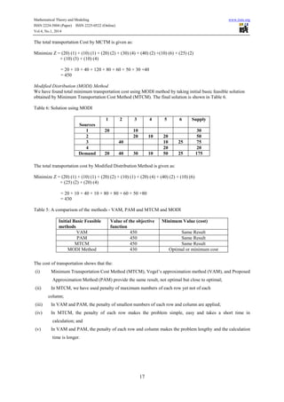
5. Conclusion
As transportation problem is a special linear programming problem having many practical applications in other
areas of operations, including, among others, inventory control, employment scheduling, and personnel
assignment as mentioned earlier. Here in our research work we have used three methods, The Minimum
Transportation Cost Method (MTCM), Vogel’s Approximation Method (VAM) and Proposed Approximation
Method (PAM). These were used to find an initial basic feasible solution for the transportation balanced model.
The results are noted to be the same. It is important to note that we have used only penalty of each row of
maximum numbers that is a simpler option and thus takes much less time in the calculation. In contrast, other
methods using maximum penalty of smallest numbers of each row and column makes the problem lengthy and
the calculation takes longer. Moreover, the method presented here is simpler in comparison of other presented
methods earlier and can be easily applied to find the initial basic feasible solution for the balanced and
unbalanced transportation problems.
REFERENCES
[1] Hamdy A Taha, Prentice Hall 2002. Operations Research: An introduction 7th Edition, p.165
[2] M.A. Hakim, An Alternative Method to Find Initial Basic Feasible Solution of a Transportation
Problem, Annals of Pure and Applied Mathematics, Vol. 1, No. 2, 2012, 203-209.
[3] S. K Goyal, Improving VAM for unbalanced transportation problems, Journal of Operational
Research Society, 35(12) (1984) 1113-1114.
[4] P. K. Gupta and Man Mohan. (1993). Linear Programming and Theory of Games, 7th edition,
Sultan Chand & Sons, New Delhi (1988) 285-318.
[5] Operations Research by Prem Kumar Gupta and D.S. Hira, Page 228-235.
[6] Goyal (1984) improving VAM for the Unbalanced Transportation Problem, Ramakrishnan
(1988) discussed some improvement to Goyal’s Modified Vogel’s Approximation method
for Unbalanced Transportation Problem.
[7] Veena Adlakha, Krzysztof Kowalski (2009), Alternate Solutions Analysis For
Transportation problems, Journal of Business & Economics Research – November,Vol 7.
[8] Sudhakar VJ, Arunnsankar N, Karpagam T (2012). A new approach for find an Optimal
Solution for Trasportation Problems, European Journal of Scientific Research 68 254-257.