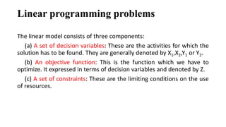
A brief study on linear programming
solving methods
Gituraj Saikia (17-12-082)
Barbie Rajkhowa (17-12-084)
Mayurjyoti Neog (17-12-095)
Group No: 15
IEOR mini-project presentation
End-semester evaluation
Introduction
 In industrial engineering, optimization is one of the most important
process.
 It is a method to determine the most favorable and best conditions for
an industrialist. It may include both maximum or minimum position.
 Linear programming is one of the method of optimizing.
 Linear modelling is one of the deterministic approach of the operation
research models.
 Linear modelling tries to maximize or minimize a linear function,
subjected to set of linear constraints.
Objectives
 To understand what linear programming is.
 To understand about types of linear programming solving systems.
 Study about how to solve linear programming problems.
Applications of Linear programming
Production planning
Distribution
Financial and economic planning
Manpower planning
Blast furnace burdening
Linear programming problems
The linear model consists of three components:
(a) A set of decision variables: These are the activities for which the
solution has to be found. They are generally denoted by X1,X2,Y1 or Y2.
(b) An objective function: This is the function which we have to
optimize. It expressed in terms of decision variables and denoted by Z.
(c) A set of constraints: These are the limiting conditions on the use
of resources.
Conditions to satisfy Linear programming
 There is a unique objective function.
 Whenever a decision variable appears in either the objective function
or in a constraint function, it must appear with a exponential 1,
possibly multiplied by a constant. So, the objective and constraint
functions must be linear.
 No terms contain product of decision variables.
 All the variables must be continuous.
 Coefficients of decision variables are constant.
 Decision variables are allowed to use integral as well as fractional
values.
Types of Linear programming models
 Generally there are two methods of solving linear programming
problems.
 First one is Graphical Method and the second one is Simplex Method.
Graphical method is one of the most basic methods to approach linear
programming problems.
A graphical interpretation proposes a number of valuable problem-solving
methods. For example, finding the greatest value of a nonstop differentiable
function ‘f(x)’ defined in some interval ‘a ≤ x ≤ b’.
We use a graphical method of linear programming for solving the problems
by finding out the maximum or lowermost point of the intersection on a
graph between the objective function line and the feasible region.
In principle, this method works for almost all different types of problems
but gets more and more difficult to solve when the number of decision
variables and the constraints increases.
1) Graphical Method
Step 1: Formulate the LP (Linear programming) problem-:This is the most
crucial step as all the subsequent steps depend on our analysis here.
Step 2: Construction of graph and plotting of the constraint lines-:The graph
must be constructed in ‘n’ dimensions , where ‘n’ is the number of decision
variables. This should give an idea about the complexity of this step if the
number of decision variables increases.
Step 3: Determination of the valid side of each constraint line-:This is used to
determine the domain of the available space, which can result in a feasible
solution.
The graphical method consists of the following steps-:
Step 4: Identification of the feasible solution region-:The feasible solution
region on the graph is the one which is satisfied by all the constraints. It could
be viewed as the intersection of the valid regions of each constraint line as
well. Choosing any point in this area would result in a valid solution for our
objective function.
Step 5: Plotting of the objective function on the graph-: One must be sure to
draw it differently from the constraint lines to avoid confusion. The constant
value in the equation of the objective function should be chosen randomly, just
to make it clearly distinguishable.
The graphical method consists of the following steps-:
Step 6: Finding the optimum point-:An optimum point always lies on one of
the corners of the feasible region.
Step 7: Finding coordinates of the optimum point-:This is the last step of the
process. This can be done by drawing two perpendicular lines from the point
onto the coordinate axes and noting down the coordinates.
The graphical method consists of the following steps-:
2)Simplex Method
• Simplex method can be used for any number of variables.
• Unlike graphical method, simplex method uses algebraic equations.
• This method can solve even those equations which have more number
of unknowns than the equations.
• Simplex procedure requires to make a table.
• Variables and constrains are entered into it and subjected to a regular
algorithm to arrive at the optimal solution.
Simplex Method Procedure
• Express the problem as an equation.
• Express the constrains of the problem as inequalities.
• Convert the inequalities to equalities by adding slack variables.
• Enter the inequalities to the simplex table.
• Complete the simplex table.
• Calculate contribution loss and net contribution and ark them on the
simplex table.
• Locate highest value of net contribution and mark it by an arrow.
• Divide the quantity column values by the corresponding values of the
column marked by an arrow and obtain the respective values.
Simplex Method Procedure
• Select the smallest non negative value amongst these values to
determine the row to be replaced.
• Compute all the values for the next row.
• Compute the values for the rest of the rows.
• Calculate contribution lost and net contribution and mark them on
simplest table.
• Repeat the steps till there is no positive value of net contribution or net
profit.
REFERENCES
1)Class notes
2)https://guides/maths/linear-programming
3)Book-: OP Khanna INDUSTRIAL ENGINEERING.
A brief study on linear programming solving methods

A brief study on linear programming solving methods

  • 1.
    A brief studyon linear programming solving methods Gituraj Saikia (17-12-082) Barbie Rajkhowa (17-12-084) Mayurjyoti Neog (17-12-095) Group No: 15 IEOR mini-project presentation End-semester evaluation
  • 2.
    Introduction  In industrialengineering, optimization is one of the most important process.  It is a method to determine the most favorable and best conditions for an industrialist. It may include both maximum or minimum position.  Linear programming is one of the method of optimizing.  Linear modelling is one of the deterministic approach of the operation research models.  Linear modelling tries to maximize or minimize a linear function, subjected to set of linear constraints.
  • 3.
    Objectives  To understandwhat linear programming is.  To understand about types of linear programming solving systems.  Study about how to solve linear programming problems.
  • 4.
    Applications of Linearprogramming Production planning Distribution Financial and economic planning Manpower planning Blast furnace burdening
  • 5.
    Linear programming problems Thelinear model consists of three components: (a) A set of decision variables: These are the activities for which the solution has to be found. They are generally denoted by X1,X2,Y1 or Y2. (b) An objective function: This is the function which we have to optimize. It expressed in terms of decision variables and denoted by Z. (c) A set of constraints: These are the limiting conditions on the use of resources.
  • 6.
    Conditions to satisfyLinear programming  There is a unique objective function.  Whenever a decision variable appears in either the objective function or in a constraint function, it must appear with a exponential 1, possibly multiplied by a constant. So, the objective and constraint functions must be linear.  No terms contain product of decision variables.  All the variables must be continuous.  Coefficients of decision variables are constant.  Decision variables are allowed to use integral as well as fractional values.
  • 7.
    Types of Linearprogramming models  Generally there are two methods of solving linear programming problems.  First one is Graphical Method and the second one is Simplex Method.
  • 8.
    Graphical method isone of the most basic methods to approach linear programming problems. A graphical interpretation proposes a number of valuable problem-solving methods. For example, finding the greatest value of a nonstop differentiable function ‘f(x)’ defined in some interval ‘a ≤ x ≤ b’. We use a graphical method of linear programming for solving the problems by finding out the maximum or lowermost point of the intersection on a graph between the objective function line and the feasible region. In principle, this method works for almost all different types of problems but gets more and more difficult to solve when the number of decision variables and the constraints increases. 1) Graphical Method
  • 9.
    Step 1: Formulatethe LP (Linear programming) problem-:This is the most crucial step as all the subsequent steps depend on our analysis here. Step 2: Construction of graph and plotting of the constraint lines-:The graph must be constructed in ‘n’ dimensions , where ‘n’ is the number of decision variables. This should give an idea about the complexity of this step if the number of decision variables increases. Step 3: Determination of the valid side of each constraint line-:This is used to determine the domain of the available space, which can result in a feasible solution. The graphical method consists of the following steps-:
  • 10.
    Step 4: Identificationof the feasible solution region-:The feasible solution region on the graph is the one which is satisfied by all the constraints. It could be viewed as the intersection of the valid regions of each constraint line as well. Choosing any point in this area would result in a valid solution for our objective function. Step 5: Plotting of the objective function on the graph-: One must be sure to draw it differently from the constraint lines to avoid confusion. The constant value in the equation of the objective function should be chosen randomly, just to make it clearly distinguishable. The graphical method consists of the following steps-:
  • 11.
    Step 6: Findingthe optimum point-:An optimum point always lies on one of the corners of the feasible region. Step 7: Finding coordinates of the optimum point-:This is the last step of the process. This can be done by drawing two perpendicular lines from the point onto the coordinate axes and noting down the coordinates. The graphical method consists of the following steps-:
  • 12.
    2)Simplex Method • Simplexmethod can be used for any number of variables. • Unlike graphical method, simplex method uses algebraic equations. • This method can solve even those equations which have more number of unknowns than the equations. • Simplex procedure requires to make a table. • Variables and constrains are entered into it and subjected to a regular algorithm to arrive at the optimal solution.
  • 13.
    Simplex Method Procedure •Express the problem as an equation. • Express the constrains of the problem as inequalities. • Convert the inequalities to equalities by adding slack variables. • Enter the inequalities to the simplex table. • Complete the simplex table. • Calculate contribution loss and net contribution and ark them on the simplex table. • Locate highest value of net contribution and mark it by an arrow. • Divide the quantity column values by the corresponding values of the column marked by an arrow and obtain the respective values.
  • 14.
    Simplex Method Procedure •Select the smallest non negative value amongst these values to determine the row to be replaced. • Compute all the values for the next row. • Compute the values for the rest of the rows. • Calculate contribution lost and net contribution and mark them on simplest table. • Repeat the steps till there is no positive value of net contribution or net profit.
  • 15.