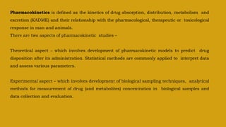
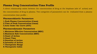
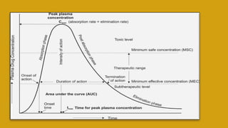
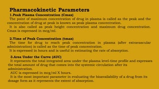
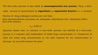
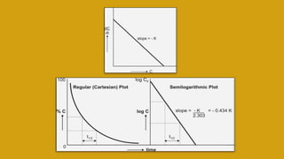
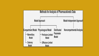
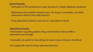
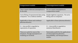
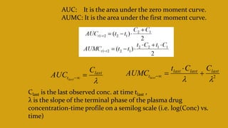
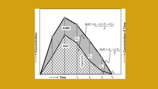
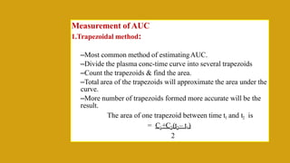
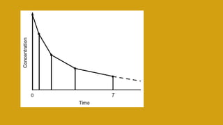
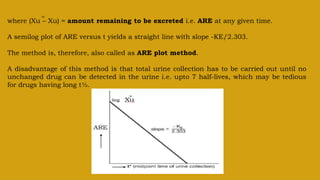
P.N.Mallikarjun
Associate Professor
Vignan Institute of Pharmaceutical Technology
PHARMACOKINETICS
Pharmacokinetics is defined as the kinetics of drug absorption, distribution, metabolism and
excretion (KADME) and their relationship with the pharmacological, therapeutic or toxicological
response in man and animals.
There are two aspects of pharmacokinetic studies –
Theoretical aspect – which involves development of pharmacokinetic models to predict drug
disposition after its administration. Statistical methods are commonly applied to interpret data
and assess various parameters.
Experimental aspect – which involves development of biological sampling techniques, analytical
methods for measurement of drug (and metabolites) concentration in biological samples and
data collection and evaluation.
Plasma Drug Concentration-Time Profile
A direct relationship exists between the concentration of drug at the biophase (site of action) and
the concentration of drug in plasma. Two categories of parameters can be evaluated from a plasma
concentration time profile –
Pharmacokinetic Parameters
1.Peak Plasma Concentration (Cmax)
2.Time of Peak Concentration (tmax)
3.Area Under the Curve (AUC)
Pharmacodynamic Parameters
1.Minimum Effective Concentration (MEC)
2.Maximum Safe Concentration (MSC)
3.Onset of Action
4.Onset Time
5.Duration of Action
6.Intensity of Action
7.Therapeutic Range
8.Therapeutic Index
Pharmacokinetic Parameters
1.Peak Plasma Concentration (Cmax)
The point of maximum concentration of drug in plasma is called as the peak and the
concentration of drug at peak is known as peak plasma concentration.
It is also called as peak height concentration and maximum drug concentration.
Cmax is expressed in mcg/ml.
2.Time of Peak Concentration (tmax)
The time for drug to reach peak concentration in plasma (after extravascular
administration) is called as the time of peak concentration.
It is expressed in hours and is useful in estimating the rate of absorption.
3.Area Under the Curve (AUC)
It represents the total integrated area under the plasma level-time profile and expresses
the total amount of drug that comes into the systemic circulation after its
administration.
AUC is expressed in mcg/ml X hours.
It is the most important parameter in evaluating the bioavailability of a drug from its
dosage form as it represents the extent of absorption.
Pharmacodynamic Parameters
1.Minimum Effective Concentration (MEC)
It is defined as the minimum concentration of drug in plasma required to produce the
therapeutic effect. It reflects the minimum concentration of drug at the receptor site to
elicit the desired pharmacological response. In case of antibiotics, the term minimum
inhibitory concentration (MIC)
2.MaximumSafeConcentration(MSC)
Also called as minimum toxic concentration (MTC), it is the concentration of drug in
plasma above which adverse or unwanted effects are precipitated.
3.Onset of Action
The beginning of pharmacological response is called as onset of action. It occurs when
the plasma drug concentration just exceeds the required MEC.
4. Onset Time
It is the time required for the drug to start producing pharmacological response. It
corresponds to the time for the plasma concentration to reach MEC after administration
of drug.
5.Duration of Action
The time period for which the plasma concentration of drug remains above the MEC
level is called as duration of drug action.
It is also defined as the difference between onset time and time for the drug to decline
back to MEC.
6.Intensity of Action
It is the maximum pharmacological response produced by the peak plasma
concentration of drug.
It is also called as peak response.
7.Therapeutic Range
The drug concentration between MEC and MSC represents the therapeutic range.
It is also known as therapeutic window.
8.Therapeutic Index
The ratio of MSC to MEC is called as therapeutic index. It is also defined as the ratio of
dose required to produce toxic or lethal effects to dose required to produce therapeutic
effect.
BASICS OF KINETICS
Rate: The velocity with which a reaction or a process occurs is called as its rate.
Order of reaction:The manner in which the concentration of drug (or reactants) influences
the rate of reaction or process is called as the order of reaction or order of process.
Consider the following chemical reaction:
Drug A Drug B
The rate of forward reaction is expressed as
-dA/dt
Negative sign indicates that the concentration of drug A decreases with time t.
As the reaction proceeds, the concentration of drug B increases and the rate of reaction can
also be expressed as: dB/dt
dC/dt = -KCn
K=Rate constant n =Order of reaction
Zero-Order Kinetics (Constant Rate Processes)
If n = 0, equation becomes:
dC/dt = -Ko Co
Where Ko = zero-order rate constant (in mg/min)
Zero-order process can be defined as the one whose rate is independent of the concentration of
drug undergoing reaction i.e. the rate of reaction cannot be increased further by increasing the
concentration of reactants.
Finally C = Co – Ko t
Zero-Order Half-Life
Half-life (t½) or half-time is defined as the time period required for the concentration of drug to
decrease by one-half.
t1/2 = Co / 2 Ko
Examples of zero-order processes are –
Administration of a drug as a constant rate i.v. infusion.
Controlled drug delivery such as that from i.m. implants or osmotic
First-Order Kinetics (Linear Kinetics)
If n = 1, equation becomes:
dC/dt = - K C
whereK = first-order rate constant (in time–1 or per hour)
first-order process is the one whose rate is directly proportional to the concentration of drug
undergoing reaction i.e. greater the concentration, faster the reaction. It is because of such
proportionality between rate of reaction and the concentration of drug that a first-order process is
said to follow linear kinetics.
ln C = ln Co - K t
Exponential form: C = C o e –Kt
log C = log Co – Kt/2.303
log C = log Co – 0.434Kt
The first-order process is also called as monoexponential rate process. Thus, a first-
order process is characterized by logarithmic or exponential kinetics i.e. a constant
fraction of drug undergoes reaction per unit time.
Most pharmacokinetic processes viz. absorption, distribution and elimination follow
first-order kinetics
t1/2 = 0.693 / K
Equation shows that, in contrast to zero-order process, the half-life of a first-order
process is a constant and independent of initial drug concentration i.e. irrespective of
what the initial drug concentration is, the time required for the concentration to
decrease by one-half remains the same.
ANALYSIS OF PHARMACOKINETIC PARAMETERS
Drug movement within the body is a complex process. The major objective is
therefore to develop a generalized and simple approach to describe, analyse and interpret
the data obtained during in vivo drug disposition studies. The two major approaches in the
quantitative study of various kinetic processes of drug disposition in the body are
1.Model approach, and
2.Model-independent approach (also called as non-compartmental analysis).
Pharmacokinetic Model Approach
A model is a hypothesis that employs mathematical terms to concisely describe
quantitative relationships. Pharmacokinetic models provide concise means of
expressing mathematically or quantitatively, the time course of drug(s) throughout the
body and compute meaningful pharmacokinetic parameters.
Types of Pharmacokinetic Models
Pharmacokinetic models are of three different types –
Compartment models – are also called as empirical models,
Physiological models – are realistic models.
Distributed parameter models – are also realistic models.
Applications of Pharmacokinetic Models –
1.Characterizing the behaviour of drugs in patients.
2.Predicting the concentration of drug in various body fluids with any dosage regimen.
3.Predicting the multiple-dose concentration curves from single dose experiments.
4.Calculating the optimum dosage regimen for individual patients.
5.Evaluating the risk of toxicity with certain dosage regimens.
6.Correlating plasma drug concentration with pharmacological response.
7.Evaluating the bioequivalence between different formulations of the same drug.
8.Estimating the possibility of drug and/or metabolite(s) accumulation in the body.
9.Determining the influence of altered physiology/disease state on drug ADME.
10.Explaining drug interactions.
Compartment Models
Compartmental analysis is the traditional and most commonly
used approach to pharmacokinetic characterization of a drug.
These models simply interpolate the experimental data and allow an
empirical formula to estimate the drug concentration with time.
Compartment is an homogeneous kinetic unit consists of all the tissues
which have similar blood flow and drug affinity.
Depending upon whether the compartments are arranged parallel or in
a series. compartment models are divided into two categories —
1.Mammillary model
2.Catenary model.
Since compartments are hypothetical in nature, compartment models are based on certain
ASSUMPTIONS –
1.The body is represented as a series of compartments arranged either in series or
parallel to each other, that communicate reversibly with each other.
2.Each compartment is not a real physiologic or anatomic region but a fictitious or
virtual one and considered as a tissue or group of tissues that have similar drug
distribution characteristics (similar blood flow and affinity).
3.Within each compartment, the drug is considered to be rapidly and uniformly
distributed i.e. the compartment is well-stirred.
4.The rate of drug movement between compartments (i.e. entry and exit) is described by
first-order kinetics.
5.Rate constants are used to represent rate of entry into and exit from the compartment.
Mammillary Model
This model is the most common compartment model used in pharmacokinetics.
The number of rate constants which will appear in a particular compartment
model is given by R.
For intravenous administration,
For extravascular administration,
where n = number of compartments.
R = 2n – 1
R = 2n
Catenary Model
Classification of compartment models
One compartment Model:
Whole body considered as one compartment. compartment is kinetically homogeneous
unit.
Two compartment Model: Body tissues are classified into 2 categories:
1.Central compartment/Compartment 1:Consist of blood and highly perfused
tissues/organs like liver, lungs,kidneys,heart etc.
2.Peripheral or Tissue compartment/Compartment 2:Consists of poorly perfused and
slow equilibrating tissues like muscles, skin, adipose tissue.
Three compartment Model :Body tissues are classified into 3 categories:
1.Central compartment/Compartment 1:Consist of blood and highly perfused
tissues/organs like liver, lungs,kidneys,heart etc.
2.Peripheral or Tissue compartment/Compartment 2: Consists of poorly perfused and
slow equilibrating tissues like muscles,skin,adipose tissue.
3.Peripheral or Tissue compartment/Compartment 3: Consists of poorly/ no perfused
tissues like bones, tissue.
ADVANTAGES:
It is a simple and flexible approach and thus widely used.
•It gives a visual representation of various rate processes
•It shows how many rate constants are necessary to describe these processes.
•It enables monitoring of drug concentration change with time with a limited amount of
data. Only plasma concentration data or urinary excretion data is sufficient.
•It is useful in predicting drug concentration-time profile in both normal physiological and
in pathological conditions.
•It is important in the development of dosage regimens.
•It is useful in relating plasma drug levels to therapeutic and toxic effects in the body.
•It is particularly useful when several therapeutic agents are compared. Clinically, drug
data comparisons are based on compartment models.
•Its simplicity allows for easy tabulation of parameters.
DISADVANTAGES:
The compartments and parameters bear no relationship with the physiological functions or
the anatomic structure of the species
•Extensive efforts are required in the development of an exact model
•The model is based on curve fitting of plasma concentration with complex multiexponential
mathematical equations.
•The model may vary within a study population.
•The approach can be applied only to a specific drug under study.
•The drug behaviour within the body may fit different compartmental models depending upon
the route of administration.
•Difficulties generally arise when using models to interpret the differences between results from
human and animal experiments.
•Owing to their simplicity, compartmental models are often misunderstood, overstretched or
even abused.
Physiological Models
These models are also known as physiologically-based pharmacokinetic models (PB-PK
models) They are drawn on the basis of known anatomic and physiological data and
thus present a more realistic picture of drug disposition in various organs and
tissues. The number of compartment to be included in the model depends upon the
disposition characteristics of the drug. Organs o tissues such as bones that have no
drug penetration are excluded.
The physiological models are further categorized into two types –
Blood flow rate-limited models – These models are more popular and commonly used
than the second type, and are based on the assumption that the drug movement within a
body region is much more rapid than its rate of delivery to that region by the perfusing
blood. These models are therefore also called as perfusion rate-limited models. This
assumption is however applicable only to the highly membrane permeable drugs i.e. low
molecular weight, poorly ionised and highly lipophilic drugs, for example, thiopental,
lidocaine, etc.
Membrane permeation rate-limited models – These models are more complex and
applicable to highly polar, ionised and charged drugs, in which case the cell membrane
acts as a barrier for the drug that gradually permeates by diffusion. These models are
therefore also called as diffusion-limited models. Owing to the time lag in equilibration
between the blood and the tissue, equations for these models are very complicated.
ADVANTAGES:Mathematical treatment is straightforward.
Data fitting is not required since drug concentration in various body regions can be predicted on
the basis of organ or tissue size, perfusion rate
The model gives exact description of drug concentration-time profile in any organ or tissue and
thus better picture of drug distribution characteristics in the body.
The influence of altered physiology or pathology on drug disposition can be easily predicted from
changes in the various pharmacokinetic parameters since the parameters correspond to actual
physiological and anatomic measures.
The method is frequently used in animals because invasive methods can be used to collect tissue
samples.
Correlation of data in several animal species is possible and with some drugs, can be extrapolated
to humans since tissue concentration of drugs is known.
Mechanism of ADME of drug can be easily explained by this model.
DISADVANTAGES: Obtaining the experimental data is a very exhaustive process.
Most physiological models assume an average blood flow for individual subjects and hence
prediction of individualized dosing is difficult.
The number of data points is less than the pharmacokinetic parameters to be assessed.
Monitoring of drug concentration in body is difficult since exhaustive data is required
Compartment Modelling Physiological Modelling
1. Hypothetical/empirical approach – no relation with
real physiology oranatomy Realistic approach since it is based on physiological
and anatomic information.
2. Experimentally simple and flexibleapproach as far
as data collection is concerned
Difficult experimentally since exhaustivedata
collection is required.
3. Owing to its simplicity, it is widely used and is often
the ―first model‖.
Less commonly used owing to complexity.
4. Complex multiexponential mathematical treatment is
necessary for curve fitting.
Mathematical treatment isstraightforward.
5. Data fitting is required for predictingdrug
concentration in a particular compartment.
Data fitting is not necessary since drugconcentration
in various tissues is practically determined.
6. Used when there is little information about the tissues. Used where tissue drug concentration and binding are
known.
7. Easy to monitor time course of drug in body with
limited data.
Exhaustive data is required to monitor time course of
drug in body.
8. Extrapolation from data to humans andvice versa is
not possible.
Extrapolation of animal data to humansis easy on the
basis of tissue concentration of drugs.
9. Mechanism of drug’s ADME cannot be explained. Easy to explain drug’s ADME mechanisms.
10. Effect of pathological condition on drug ADME
cannot be determined.
Effect of pathology on drug ADME can be easily
determined.
MODEL INDEPENDENT METHOD-
NON COMPARTMENTAL ANALYSIS:
The noncompartmental approach is a new approach devised to study the time
course of drug in the body with out assuming any compartment model.
The noncompartmental approach for data analysis does not require any
specific compartmental model for the system (body) and can be applied to virtually
any pharmacokinetic data.
NonCompartmental Analysis(NCA) is a Model independent method.
NCA Overcomes some of the drawbacks associated with classical
compartment modeling.
Basic assumption is that drug or metabolite follows first-order kinetics.
Based on the statistical moment theory.
APPLICATIONS:
•The main purpose of the noncompartmental approach is to estimate various
pharmacokinetic parameters, such as systemic clearance, volume of distribution
at steady state, mean residence time, and bioavailability without assuming or
understanding any structural or mechanistic properties of the pharmacokinetic
behavior of a drug in the body
•In addition, many noncompartmental methods allow the estimation of those
pharmacokinetic parameters from drug concentration profiles without the
complicated, and often subjective, nonlinear regression processes required for
the compartmental models
•Owing to this versatility and ruggedness, the noncompartmental approach is a
primary pharmacokinetic data analysis method for the pharmaceutical industry.
ADVANTAGES:
 Derivation of PK parameters is easy, because of simple algebraic equations
 Mathematical treatment remains same, for drug or metabolite, provided
elimination follows first order kinetics
 Drug disposition kinetics need not be described in detail
DISADVANTAGES:
•Information regarding plasma drug concentration-time profile is
expressed as an average
•Generally not useful for describing the time course of drug in the blood
•It is applicable only for linear pharmacokinetics
Compartment models Noncompartment models
These require elaborate assumptions to
fit the data
Do not require assumptions to
compartment model.
Curve fitting of experimental data using
computers. It is a tedious method.
Simple algebraic equations. No curve
fitting and no computers
Applicable to linear and nonlinear
pharmacokinetics
Applicable to linear pharmacokinetics.
C1 - time profile is regarded as
expressions of exponents
C1 – time profile is regarded as
statistical distribution.
These are useful for most of the
situations, though assumptions of
modeling are involved.
Particularly useful for the applications
of clinical pharmacokinetics,
bioavailability, and bioequivalence
studies.
statistical moment theory: Suppose one could observe a single molecule,
from the time it is administered into the body ( t = 0) until it is eventually
eliminated ( t = tel ). Clearly, tel is not predictable
This individual molecule could be eliminated during the first minute or could
reside in the body for weeks.If, however, one looks at a large number of
molecules collectively, their behavior appears much more regular
The collective, or mean time of residence, of all the molecules in the dose, is
called the mean residence time (MRT).
number of molecules ,n1 and spending a different residence time , t1 .
The mean residence time (MRT) is the average time the total number of
molecules introduced (N) reside in the body.
MRT=
MRT=
MRT=







0
0
).
(
).
(
dt
t
C
dt
t
C
t
AUC
AUMC
MRT
MRT is a mean time interval during which a drug molecule resides in the
body before being excreted
AUC: It is the area under the zero moment curve.
AUMC: It is the area under the first moment curve.

last
t
C
AUClast


 2


last
last
last
t
C
C
t
AUMClast





Clast is the last observed conc. at time tlast ,
λ is the slope of the terminal phase of the plasma drug
concentration-time profile on a semilog scale (i.e. log(Conc) vs.
time)
Measurement of AUC
1.Trapezoidal method:
–Most common method of estimatingAUC.
–Divide the plasma conc-time curve into several trapezoids
–Count the trapezoids & find the area.
–Total area of the trapezoids will approximate the area under the
curve.
–More number of trapezoids formed more accurate will be the
result.
The area of one trapezoid between time t1 and t2 is
= C1+C2(t2– t1)
2
• Preparing calibrated Plasma level time profile curve on a equal
density paper and is cut and weigh the curve.
• Sample curve is cut & weight is recorded.
• By interpolation method area of sample graph is found.
Instrument for mechanically measuring the
area under the curve
Measures area by tracing outline of curve.
Disadvantage:
Degree of error is high due to
instrumental& human error.
2.CUT & WEIGH METHOD:
3.PLANIMETER:
Total no. of squares enclosed in the curve is counted.
Area of each square determined using relationship:
AREA=(height) (width)
4.COUNTING THE SQUARE :
NON INVASIVE METHODS OF ANALYSIS:
URINE EXCRETION DATA
In the absence of plasma level-time data, useful information can still be
obtained from urine/saliva data regarding elimination kinetics of a drug.
The method has several advantages in the analysis of a pharmacokinetic
system:
1.The method is useful when there is lack of sufficiently sensitive analytical
techniques to measure concentration of drugs in plasma with accuracy.
2.The method is non-invasive and therefore better subject compliance is
assured.
3.A less sensitive analytical method is required for determining
urine drug concentration as compared to plasma concentrations.
If urine drug concentrations are low, assaying of larger sample
volumes is relatively easy.
4.First-order elimination, excretion and absorption rate constants
and fraction excreted unchanged can be computed from such
data. First-order metabolism or extra-renal excretion rate constant
can also be calculated subsequently from the difference (KE – Ke)
= Km.
5.Direct measurement of bioavailability, both absolute and
relative, is possible without the necessity of fitting the data to a
mathematical model.
Criteria for Obtaining Valid Urinary Excretion Data
1.A significant amount of drug must be excreted unchanged in the
urine (at least 10%).
2.The analytical method must be specific for the unchanged drug;
metabolites should not interfere.
3.Water-loading should be done by taking 400 ml of water after
fasting overnight, to promote diuresis and enable collection of
sufficient urine samples.
4.Before administration of drug, the bladder must be emptied
completely after 1 hour from water-loading and the urine sample
taken as blank. The drug should then be administered with 200 ml
of water and should be followed by 200 ml given at hourly intervals
for the next 4 hours.
5.Volunteers must be instructed to completely empty their bladder
while collecting urine samples.
6.Frequent sampling should be done in order to obtain a good curve.
7.During sampling, the exact time and volume of urine excreted should
be noted.
8.An individual collection period should not exceed one biological half-
life of the drug and ideally should be considerably less.
9.Urine samples must be collected for at least 7 biological half-lives in
order to ensure collection of more than 99% of excreted drug.
10.Changes in urine pH and urine volume may alter the urinary
excretion rate.
dXu
dt
 K e X
Determination of KE & Ke from Urinary Excretion Data
The first-order elimination (and excretion) rate constants can be computed from
urine data by two methods:
• Rate of excretion method, and
• Sigma-minus method.
Rate of Excretion Method: The rate of urinary drug excretion dXu/dt is proportional to
the amount of drug in the body X and written as:
According to first-order disposition kinetics, X = Xo e–KEt
dXu
dt
 K e Xo e–KEt
log Ke X0 -
dXu
dt
KEt
2.303
log
Sigma-Minus Method:
A disadvantage of rate of excretion method in estimating KE is that fluctuations in the rate of drug
elimination are observed to a high degree and in most instances, the data are so scattered that an estimate
of half-life is difficult. These problems can be minimized by using the alternative approach called as
sigma-minus method.
dXu
dt
Xo e–KEt
 K e
Xu 
Ke X0
KE
(1 - e-K E t
)
Xu = cumulative amount of drug excreted unchanged in urine at any time t. As time approaches
infinity i.e. after 6 to 7 half-lives, the value e–KE∞ becomes zero and therefore the cumulative
amount excreted at infinite time Xu ∞ can be given by equation
X u - X u  X u e–KEt
X u

 

Ke X0
KE
l o g ( X u – X u )  logX u -

2.303
KEt

where (Xu – Xu) = amount remaining to be excreted i.e. ARE at any given time.
A semilog plot of ARE versus t yields a straight line with slope -KE/2.303.
The method is, therefore, also called as ARE plot method.
A disadvantage of this method is that total urine collection has to be carried out until no
unchanged drug can be detected in the urine i.e. upto 7 half-lives, which may be tedious
for drugs having long t½.
ARE
Xu


1.pharmacokinetics

  • 1.
    P.N.Mallikarjun Associate Professor Vignan Instituteof Pharmaceutical Technology PHARMACOKINETICS
  • 3.
    Pharmacokinetics is definedas the kinetics of drug absorption, distribution, metabolism and excretion (KADME) and their relationship with the pharmacological, therapeutic or toxicological response in man and animals. There are two aspects of pharmacokinetic studies – Theoretical aspect – which involves development of pharmacokinetic models to predict drug disposition after its administration. Statistical methods are commonly applied to interpret data and assess various parameters. Experimental aspect – which involves development of biological sampling techniques, analytical methods for measurement of drug (and metabolites) concentration in biological samples and data collection and evaluation.
  • 4.
    Plasma Drug Concentration-TimeProfile A direct relationship exists between the concentration of drug at the biophase (site of action) and the concentration of drug in plasma. Two categories of parameters can be evaluated from a plasma concentration time profile – Pharmacokinetic Parameters 1.Peak Plasma Concentration (Cmax) 2.Time of Peak Concentration (tmax) 3.Area Under the Curve (AUC) Pharmacodynamic Parameters 1.Minimum Effective Concentration (MEC) 2.Maximum Safe Concentration (MSC) 3.Onset of Action 4.Onset Time 5.Duration of Action 6.Intensity of Action 7.Therapeutic Range 8.Therapeutic Index
  • 6.
    Pharmacokinetic Parameters 1.Peak PlasmaConcentration (Cmax) The point of maximum concentration of drug in plasma is called as the peak and the concentration of drug at peak is known as peak plasma concentration. It is also called as peak height concentration and maximum drug concentration. Cmax is expressed in mcg/ml. 2.Time of Peak Concentration (tmax) The time for drug to reach peak concentration in plasma (after extravascular administration) is called as the time of peak concentration. It is expressed in hours and is useful in estimating the rate of absorption. 3.Area Under the Curve (AUC) It represents the total integrated area under the plasma level-time profile and expresses the total amount of drug that comes into the systemic circulation after its administration. AUC is expressed in mcg/ml X hours. It is the most important parameter in evaluating the bioavailability of a drug from its dosage form as it represents the extent of absorption.
  • 7.
    Pharmacodynamic Parameters 1.Minimum EffectiveConcentration (MEC) It is defined as the minimum concentration of drug in plasma required to produce the therapeutic effect. It reflects the minimum concentration of drug at the receptor site to elicit the desired pharmacological response. In case of antibiotics, the term minimum inhibitory concentration (MIC) 2.MaximumSafeConcentration(MSC) Also called as minimum toxic concentration (MTC), it is the concentration of drug in plasma above which adverse or unwanted effects are precipitated. 3.Onset of Action The beginning of pharmacological response is called as onset of action. It occurs when the plasma drug concentration just exceeds the required MEC. 4. Onset Time It is the time required for the drug to start producing pharmacological response. It corresponds to the time for the plasma concentration to reach MEC after administration of drug.
  • 8.
    5.Duration of Action Thetime period for which the plasma concentration of drug remains above the MEC level is called as duration of drug action. It is also defined as the difference between onset time and time for the drug to decline back to MEC. 6.Intensity of Action It is the maximum pharmacological response produced by the peak plasma concentration of drug. It is also called as peak response. 7.Therapeutic Range The drug concentration between MEC and MSC represents the therapeutic range. It is also known as therapeutic window. 8.Therapeutic Index The ratio of MSC to MEC is called as therapeutic index. It is also defined as the ratio of dose required to produce toxic or lethal effects to dose required to produce therapeutic effect.
  • 9.
    BASICS OF KINETICS Rate:The velocity with which a reaction or a process occurs is called as its rate. Order of reaction:The manner in which the concentration of drug (or reactants) influences the rate of reaction or process is called as the order of reaction or order of process. Consider the following chemical reaction: Drug A Drug B The rate of forward reaction is expressed as -dA/dt Negative sign indicates that the concentration of drug A decreases with time t. As the reaction proceeds, the concentration of drug B increases and the rate of reaction can also be expressed as: dB/dt dC/dt = -KCn K=Rate constant n =Order of reaction
  • 10.
    Zero-Order Kinetics (ConstantRate Processes) If n = 0, equation becomes: dC/dt = -Ko Co Where Ko = zero-order rate constant (in mg/min) Zero-order process can be defined as the one whose rate is independent of the concentration of drug undergoing reaction i.e. the rate of reaction cannot be increased further by increasing the concentration of reactants. Finally C = Co – Ko t Zero-Order Half-Life Half-life (t½) or half-time is defined as the time period required for the concentration of drug to decrease by one-half. t1/2 = Co / 2 Ko Examples of zero-order processes are – Administration of a drug as a constant rate i.v. infusion. Controlled drug delivery such as that from i.m. implants or osmotic
  • 12.
    First-Order Kinetics (LinearKinetics) If n = 1, equation becomes: dC/dt = - K C whereK = first-order rate constant (in time–1 or per hour) first-order process is the one whose rate is directly proportional to the concentration of drug undergoing reaction i.e. greater the concentration, faster the reaction. It is because of such proportionality between rate of reaction and the concentration of drug that a first-order process is said to follow linear kinetics. ln C = ln Co - K t Exponential form: C = C o e –Kt log C = log Co – Kt/2.303 log C = log Co – 0.434Kt
  • 13.
    The first-order processis also called as monoexponential rate process. Thus, a first- order process is characterized by logarithmic or exponential kinetics i.e. a constant fraction of drug undergoes reaction per unit time. Most pharmacokinetic processes viz. absorption, distribution and elimination follow first-order kinetics t1/2 = 0.693 / K Equation shows that, in contrast to zero-order process, the half-life of a first-order process is a constant and independent of initial drug concentration i.e. irrespective of what the initial drug concentration is, the time required for the concentration to decrease by one-half remains the same.
  • 15.
    ANALYSIS OF PHARMACOKINETICPARAMETERS Drug movement within the body is a complex process. The major objective is therefore to develop a generalized and simple approach to describe, analyse and interpret the data obtained during in vivo drug disposition studies. The two major approaches in the quantitative study of various kinetic processes of drug disposition in the body are 1.Model approach, and 2.Model-independent approach (also called as non-compartmental analysis).
  • 17.
    Pharmacokinetic Model Approach Amodel is a hypothesis that employs mathematical terms to concisely describe quantitative relationships. Pharmacokinetic models provide concise means of expressing mathematically or quantitatively, the time course of drug(s) throughout the body and compute meaningful pharmacokinetic parameters. Types of Pharmacokinetic Models Pharmacokinetic models are of three different types – Compartment models – are also called as empirical models, Physiological models – are realistic models. Distributed parameter models – are also realistic models.
  • 18.
    Applications of PharmacokineticModels – 1.Characterizing the behaviour of drugs in patients. 2.Predicting the concentration of drug in various body fluids with any dosage regimen. 3.Predicting the multiple-dose concentration curves from single dose experiments. 4.Calculating the optimum dosage regimen for individual patients. 5.Evaluating the risk of toxicity with certain dosage regimens. 6.Correlating plasma drug concentration with pharmacological response. 7.Evaluating the bioequivalence between different formulations of the same drug. 8.Estimating the possibility of drug and/or metabolite(s) accumulation in the body. 9.Determining the influence of altered physiology/disease state on drug ADME. 10.Explaining drug interactions.
  • 19.
    Compartment Models Compartmental analysisis the traditional and most commonly used approach to pharmacokinetic characterization of a drug. These models simply interpolate the experimental data and allow an empirical formula to estimate the drug concentration with time. Compartment is an homogeneous kinetic unit consists of all the tissues which have similar blood flow and drug affinity. Depending upon whether the compartments are arranged parallel or in a series. compartment models are divided into two categories — 1.Mammillary model 2.Catenary model.
  • 20.
    Since compartments arehypothetical in nature, compartment models are based on certain ASSUMPTIONS – 1.The body is represented as a series of compartments arranged either in series or parallel to each other, that communicate reversibly with each other. 2.Each compartment is not a real physiologic or anatomic region but a fictitious or virtual one and considered as a tissue or group of tissues that have similar drug distribution characteristics (similar blood flow and affinity). 3.Within each compartment, the drug is considered to be rapidly and uniformly distributed i.e. the compartment is well-stirred. 4.The rate of drug movement between compartments (i.e. entry and exit) is described by first-order kinetics. 5.Rate constants are used to represent rate of entry into and exit from the compartment.
  • 21.
    Mammillary Model This modelis the most common compartment model used in pharmacokinetics.
  • 22.
    The number ofrate constants which will appear in a particular compartment model is given by R. For intravenous administration, For extravascular administration, where n = number of compartments. R = 2n – 1 R = 2n Catenary Model
  • 23.
    Classification of compartmentmodels One compartment Model: Whole body considered as one compartment. compartment is kinetically homogeneous unit. Two compartment Model: Body tissues are classified into 2 categories: 1.Central compartment/Compartment 1:Consist of blood and highly perfused tissues/organs like liver, lungs,kidneys,heart etc. 2.Peripheral or Tissue compartment/Compartment 2:Consists of poorly perfused and slow equilibrating tissues like muscles, skin, adipose tissue. Three compartment Model :Body tissues are classified into 3 categories: 1.Central compartment/Compartment 1:Consist of blood and highly perfused tissues/organs like liver, lungs,kidneys,heart etc. 2.Peripheral or Tissue compartment/Compartment 2: Consists of poorly perfused and slow equilibrating tissues like muscles,skin,adipose tissue. 3.Peripheral or Tissue compartment/Compartment 3: Consists of poorly/ no perfused tissues like bones, tissue.
  • 24.
    ADVANTAGES: It is asimple and flexible approach and thus widely used. •It gives a visual representation of various rate processes •It shows how many rate constants are necessary to describe these processes. •It enables monitoring of drug concentration change with time with a limited amount of data. Only plasma concentration data or urinary excretion data is sufficient. •It is useful in predicting drug concentration-time profile in both normal physiological and in pathological conditions. •It is important in the development of dosage regimens. •It is useful in relating plasma drug levels to therapeutic and toxic effects in the body. •It is particularly useful when several therapeutic agents are compared. Clinically, drug data comparisons are based on compartment models. •Its simplicity allows for easy tabulation of parameters.
  • 25.
    DISADVANTAGES: The compartments andparameters bear no relationship with the physiological functions or the anatomic structure of the species •Extensive efforts are required in the development of an exact model •The model is based on curve fitting of plasma concentration with complex multiexponential mathematical equations. •The model may vary within a study population. •The approach can be applied only to a specific drug under study. •The drug behaviour within the body may fit different compartmental models depending upon the route of administration. •Difficulties generally arise when using models to interpret the differences between results from human and animal experiments. •Owing to their simplicity, compartmental models are often misunderstood, overstretched or even abused.
  • 26.
    Physiological Models These modelsare also known as physiologically-based pharmacokinetic models (PB-PK models) They are drawn on the basis of known anatomic and physiological data and thus present a more realistic picture of drug disposition in various organs and tissues. The number of compartment to be included in the model depends upon the disposition characteristics of the drug. Organs o tissues such as bones that have no drug penetration are excluded.
  • 28.
    The physiological modelsare further categorized into two types – Blood flow rate-limited models – These models are more popular and commonly used than the second type, and are based on the assumption that the drug movement within a body region is much more rapid than its rate of delivery to that region by the perfusing blood. These models are therefore also called as perfusion rate-limited models. This assumption is however applicable only to the highly membrane permeable drugs i.e. low molecular weight, poorly ionised and highly lipophilic drugs, for example, thiopental, lidocaine, etc. Membrane permeation rate-limited models – These models are more complex and applicable to highly polar, ionised and charged drugs, in which case the cell membrane acts as a barrier for the drug that gradually permeates by diffusion. These models are therefore also called as diffusion-limited models. Owing to the time lag in equilibration between the blood and the tissue, equations for these models are very complicated.
  • 29.
    ADVANTAGES:Mathematical treatment isstraightforward. Data fitting is not required since drug concentration in various body regions can be predicted on the basis of organ or tissue size, perfusion rate The model gives exact description of drug concentration-time profile in any organ or tissue and thus better picture of drug distribution characteristics in the body. The influence of altered physiology or pathology on drug disposition can be easily predicted from changes in the various pharmacokinetic parameters since the parameters correspond to actual physiological and anatomic measures. The method is frequently used in animals because invasive methods can be used to collect tissue samples. Correlation of data in several animal species is possible and with some drugs, can be extrapolated to humans since tissue concentration of drugs is known. Mechanism of ADME of drug can be easily explained by this model. DISADVANTAGES: Obtaining the experimental data is a very exhaustive process. Most physiological models assume an average blood flow for individual subjects and hence prediction of individualized dosing is difficult. The number of data points is less than the pharmacokinetic parameters to be assessed. Monitoring of drug concentration in body is difficult since exhaustive data is required
  • 30.
    Compartment Modelling PhysiologicalModelling 1. Hypothetical/empirical approach – no relation with real physiology oranatomy Realistic approach since it is based on physiological and anatomic information. 2. Experimentally simple and flexibleapproach as far as data collection is concerned Difficult experimentally since exhaustivedata collection is required. 3. Owing to its simplicity, it is widely used and is often the ―first model‖. Less commonly used owing to complexity. 4. Complex multiexponential mathematical treatment is necessary for curve fitting. Mathematical treatment isstraightforward. 5. Data fitting is required for predictingdrug concentration in a particular compartment. Data fitting is not necessary since drugconcentration in various tissues is practically determined. 6. Used when there is little information about the tissues. Used where tissue drug concentration and binding are known. 7. Easy to monitor time course of drug in body with limited data. Exhaustive data is required to monitor time course of drug in body. 8. Extrapolation from data to humans andvice versa is not possible. Extrapolation of animal data to humansis easy on the basis of tissue concentration of drugs. 9. Mechanism of drug’s ADME cannot be explained. Easy to explain drug’s ADME mechanisms. 10. Effect of pathological condition on drug ADME cannot be determined. Effect of pathology on drug ADME can be easily determined.
  • 31.
    MODEL INDEPENDENT METHOD- NONCOMPARTMENTAL ANALYSIS: The noncompartmental approach is a new approach devised to study the time course of drug in the body with out assuming any compartment model. The noncompartmental approach for data analysis does not require any specific compartmental model for the system (body) and can be applied to virtually any pharmacokinetic data. NonCompartmental Analysis(NCA) is a Model independent method. NCA Overcomes some of the drawbacks associated with classical compartment modeling. Basic assumption is that drug or metabolite follows first-order kinetics. Based on the statistical moment theory.
  • 32.
    APPLICATIONS: •The main purposeof the noncompartmental approach is to estimate various pharmacokinetic parameters, such as systemic clearance, volume of distribution at steady state, mean residence time, and bioavailability without assuming or understanding any structural or mechanistic properties of the pharmacokinetic behavior of a drug in the body •In addition, many noncompartmental methods allow the estimation of those pharmacokinetic parameters from drug concentration profiles without the complicated, and often subjective, nonlinear regression processes required for the compartmental models •Owing to this versatility and ruggedness, the noncompartmental approach is a primary pharmacokinetic data analysis method for the pharmaceutical industry.
  • 33.
    ADVANTAGES:  Derivation ofPK parameters is easy, because of simple algebraic equations  Mathematical treatment remains same, for drug or metabolite, provided elimination follows first order kinetics  Drug disposition kinetics need not be described in detail DISADVANTAGES: •Information regarding plasma drug concentration-time profile is expressed as an average •Generally not useful for describing the time course of drug in the blood •It is applicable only for linear pharmacokinetics
  • 34.
    Compartment models Noncompartmentmodels These require elaborate assumptions to fit the data Do not require assumptions to compartment model. Curve fitting of experimental data using computers. It is a tedious method. Simple algebraic equations. No curve fitting and no computers Applicable to linear and nonlinear pharmacokinetics Applicable to linear pharmacokinetics. C1 - time profile is regarded as expressions of exponents C1 – time profile is regarded as statistical distribution. These are useful for most of the situations, though assumptions of modeling are involved. Particularly useful for the applications of clinical pharmacokinetics, bioavailability, and bioequivalence studies.
  • 35.
    statistical moment theory:Suppose one could observe a single molecule, from the time it is administered into the body ( t = 0) until it is eventually eliminated ( t = tel ). Clearly, tel is not predictable This individual molecule could be eliminated during the first minute or could reside in the body for weeks.If, however, one looks at a large number of molecules collectively, their behavior appears much more regular The collective, or mean time of residence, of all the molecules in the dose, is called the mean residence time (MRT). number of molecules ,n1 and spending a different residence time , t1 . The mean residence time (MRT) is the average time the total number of molecules introduced (N) reside in the body. MRT=
  • 36.
    MRT= MRT=        0 0 ). ( ). ( dt t C dt t C t AUC AUMC MRT MRT is amean time interval during which a drug molecule resides in the body before being excreted
  • 37.
    AUC: It isthe area under the zero moment curve. AUMC: It is the area under the first moment curve.  last t C AUClast    2   last last last t C C t AUMClast      Clast is the last observed conc. at time tlast , λ is the slope of the terminal phase of the plasma drug concentration-time profile on a semilog scale (i.e. log(Conc) vs. time)
  • 39.
    Measurement of AUC 1.Trapezoidalmethod: –Most common method of estimatingAUC. –Divide the plasma conc-time curve into several trapezoids –Count the trapezoids & find the area. –Total area of the trapezoids will approximate the area under the curve. –More number of trapezoids formed more accurate will be the result. The area of one trapezoid between time t1 and t2 is = C1+C2(t2– t1) 2
  • 41.
    • Preparing calibratedPlasma level time profile curve on a equal density paper and is cut and weigh the curve. • Sample curve is cut & weight is recorded. • By interpolation method area of sample graph is found. Instrument for mechanically measuring the area under the curve Measures area by tracing outline of curve. Disadvantage: Degree of error is high due to instrumental& human error. 2.CUT & WEIGH METHOD: 3.PLANIMETER:
  • 42.
    Total no. ofsquares enclosed in the curve is counted. Area of each square determined using relationship: AREA=(height) (width) 4.COUNTING THE SQUARE :
  • 43.
    NON INVASIVE METHODSOF ANALYSIS: URINE EXCRETION DATA In the absence of plasma level-time data, useful information can still be obtained from urine/saliva data regarding elimination kinetics of a drug. The method has several advantages in the analysis of a pharmacokinetic system: 1.The method is useful when there is lack of sufficiently sensitive analytical techniques to measure concentration of drugs in plasma with accuracy. 2.The method is non-invasive and therefore better subject compliance is assured.
  • 44.
    3.A less sensitiveanalytical method is required for determining urine drug concentration as compared to plasma concentrations. If urine drug concentrations are low, assaying of larger sample volumes is relatively easy. 4.First-order elimination, excretion and absorption rate constants and fraction excreted unchanged can be computed from such data. First-order metabolism or extra-renal excretion rate constant can also be calculated subsequently from the difference (KE – Ke) = Km. 5.Direct measurement of bioavailability, both absolute and relative, is possible without the necessity of fitting the data to a mathematical model.
  • 45.
    Criteria for ObtainingValid Urinary Excretion Data 1.A significant amount of drug must be excreted unchanged in the urine (at least 10%). 2.The analytical method must be specific for the unchanged drug; metabolites should not interfere. 3.Water-loading should be done by taking 400 ml of water after fasting overnight, to promote diuresis and enable collection of sufficient urine samples. 4.Before administration of drug, the bladder must be emptied completely after 1 hour from water-loading and the urine sample taken as blank. The drug should then be administered with 200 ml of water and should be followed by 200 ml given at hourly intervals for the next 4 hours.
  • 46.
    5.Volunteers must beinstructed to completely empty their bladder while collecting urine samples. 6.Frequent sampling should be done in order to obtain a good curve. 7.During sampling, the exact time and volume of urine excreted should be noted. 8.An individual collection period should not exceed one biological half- life of the drug and ideally should be considerably less. 9.Urine samples must be collected for at least 7 biological half-lives in order to ensure collection of more than 99% of excreted drug. 10.Changes in urine pH and urine volume may alter the urinary excretion rate.
  • 47.
    dXu dt  K eX Determination of KE & Ke from Urinary Excretion Data The first-order elimination (and excretion) rate constants can be computed from urine data by two methods: • Rate of excretion method, and • Sigma-minus method. Rate of Excretion Method: The rate of urinary drug excretion dXu/dt is proportional to the amount of drug in the body X and written as: According to first-order disposition kinetics, X = Xo e–KEt dXu dt  K e Xo e–KEt log Ke X0 - dXu dt KEt 2.303 log
  • 48.
    Sigma-Minus Method: A disadvantageof rate of excretion method in estimating KE is that fluctuations in the rate of drug elimination are observed to a high degree and in most instances, the data are so scattered that an estimate of half-life is difficult. These problems can be minimized by using the alternative approach called as sigma-minus method. dXu dt Xo e–KEt  K e Xu  Ke X0 KE (1 - e-K E t ) Xu = cumulative amount of drug excreted unchanged in urine at any time t. As time approaches infinity i.e. after 6 to 7 half-lives, the value e–KE∞ becomes zero and therefore the cumulative amount excreted at infinite time Xu ∞ can be given by equation X u - X u  X u e–KEt X u     Ke X0 KE l o g ( X u – X u )  logX u -  2.303 KEt 
  • 49.
    where (Xu –Xu) = amount remaining to be excreted i.e. ARE at any given time. A semilog plot of ARE versus t yields a straight line with slope -KE/2.303. The method is, therefore, also called as ARE plot method. A disadvantage of this method is that total urine collection has to be carried out until no unchanged drug can be detected in the urine i.e. upto 7 half-lives, which may be tedious for drugs having long t½. ARE Xu 