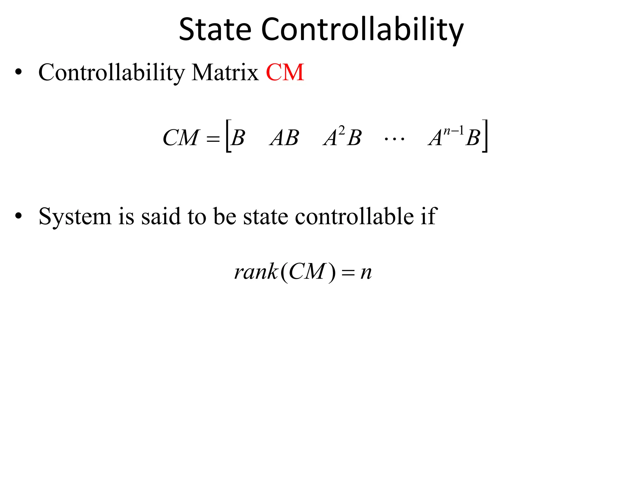
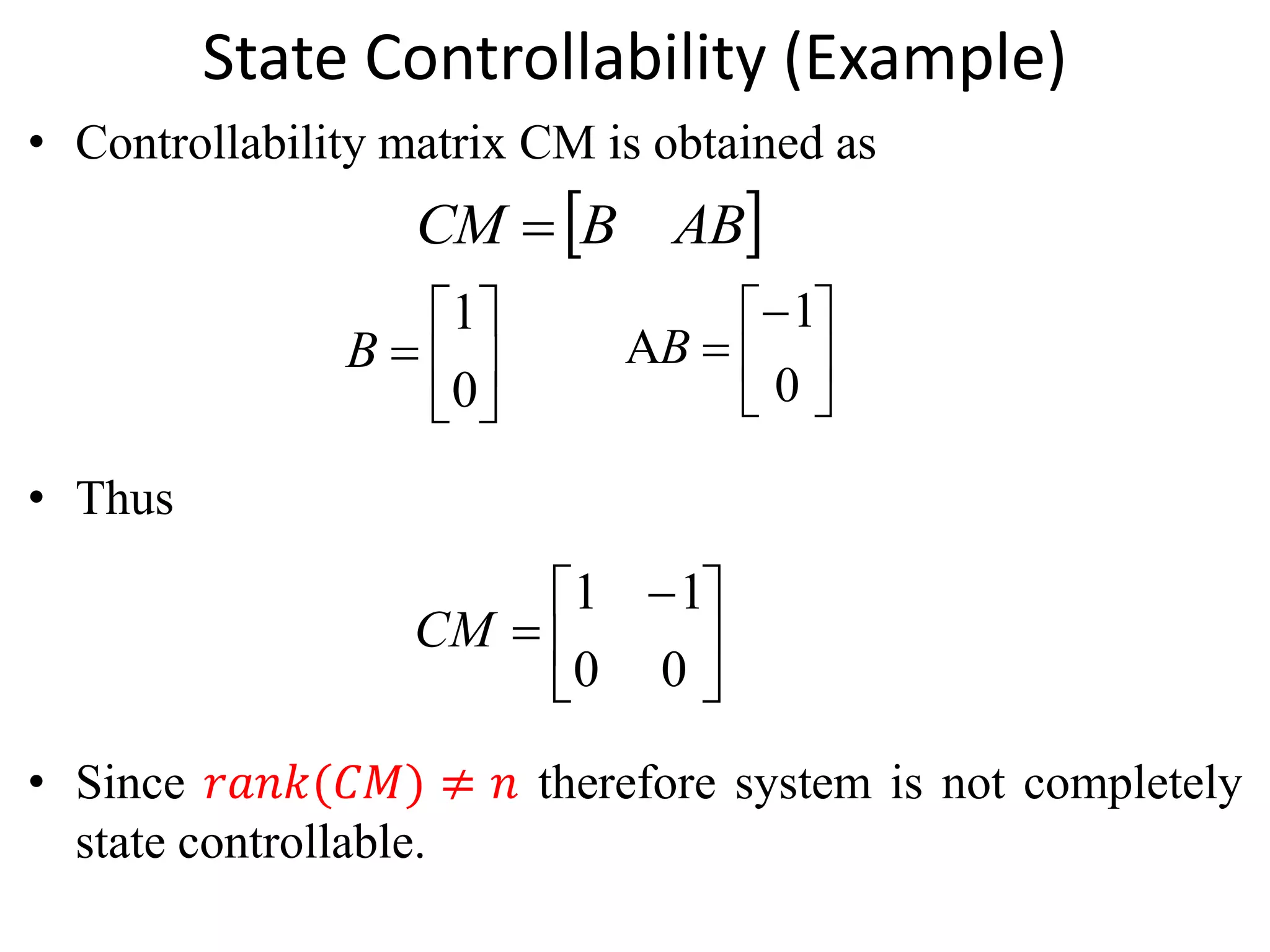
Modern Control Systems (MCS)
Dr. Imtiaz Hussain
email: imtiaz.hussain@faculty.muet.edu.pk
URL :http://imtiazhussainkalwar.weebly.com/
Lecture-13
Introduction to State Space Modeling & Analysis
Lecture Outline
• Introduction to state space
– Basic Definitions
– State Equations
– State Diagram
– State Controllability
– State Observability
– Output Controllability
Introduction
• Modern control theory is contrasted with conventional
control theory in that the former is applicable to
multiple-input, multiple-output systems, which may be
linear or nonlinear, time invariant or time varying, while
the latter is applicable only to linear time invariant single-
input, single-output systems.
Definitions
• State of a system: We define the state of a system at time t0 as
the amount of information that must be provided at time t0,
which, together with the input signal u(t) for t  t0, uniquely
determine the output of the system for all t  t0.
• State Variable: The state variables of a dynamic system are the
smallest set of variables that determine the state of the
dynamic system.
• State Vector: If n variables are needed to completely describe
the behaviour of the dynamic system then n variables can be
considered as n components of a vector x, such a vector is called
state vector.
• State Space: The state space is defined as the n-dimensional
space in which the components of the state vector represents
its coordinate axes.
Definitions
• Let x1 and x2 are two states variables that define the state
of the system completely .
5
1
x
2
x
Two Dimensional State space
State (t=t1)
State
Vector
x
dt
dx
State space of a Vehicle
Velocity
Position
State (t=t1)
State Space Equations
• In state-space analysis we are concerned with three types of
variables that are involved in the modeling of dynamic systems:
input variables, output variables, and state variables.
• The dynamic system must involve elements that memorize the
values of the input for t> t1 .
• Since integrators in a continuous-time control system serve as
memory devices, the outputs of such integrators can be
considered as the variables that define the internal state of the
dynamic system.
• Thus the outputs of integrators serve as state variables.
• The number of state variables to completely define the dynamics
of the system is equal to the number of integrators involved in the
system.
State Space Equations
• Assume that a multiple-input, multiple-output system involves 𝑛
integrators.
• Assume also that there are 𝑟 inputs 𝑢1 𝑡 , 𝑢2 𝑡 , ⋯ , 𝑢𝑟 𝑡 and 𝑚
outputs 𝑦1 𝑡 , 𝑦2 𝑡 , ⋯ , 𝑦𝑚 𝑡 .
• Define 𝑛 outputs of the integrators as state variables:
𝑥1 𝑡 , 𝑥2 𝑡 , ⋯ , 𝑥𝑛 𝑡 .
• Then the system may be described by
𝑥1 𝑡 = 𝑓1(𝑥1, 𝑥2, ⋯ , 𝑥𝑛; 𝑢1, 𝑢2, ⋯ , 𝑢𝑟; 𝑡)
𝑥2 𝑡 = 𝑓2(𝑥1, 𝑥2, ⋯ , 𝑥𝑛; 𝑢1, 𝑢2, ⋯ , 𝑢𝑟; 𝑡)
𝑥𝑛 𝑡 = 𝑓𝑛(𝑥1, 𝑥2, ⋯ , 𝑥𝑛; 𝑢1, 𝑢2, ⋯ , 𝑢𝑟; 𝑡)
State Space Equations
• The outputs 𝑦1 𝑡 , 𝑦2 𝑡 , ⋯ , 𝑦𝑚 𝑡 of the system may be given as.
• If we define
𝑦1 𝑡 = 𝑔1(𝑥1, 𝑥2, ⋯ , 𝑥𝑛; 𝑢1, 𝑢2, ⋯ , 𝑢𝑟; 𝑡)
𝑦2 𝑡 = 𝑔2(𝑥1, 𝑥2, ⋯ , 𝑥𝑛; 𝑢1, 𝑢2, ⋯ , 𝑢𝑟; 𝑡)
𝑦𝑚 𝑡 = 𝑔𝑚(𝑥1, 𝑥2, ⋯ , 𝑥𝑛; 𝑢1, 𝑢2, ⋯ , 𝑢𝑟; 𝑡)
𝒙 𝑡 =
𝑥1
𝑥2
⋮
𝑥𝑛
𝒇 𝒙, 𝒖, 𝑡 =
𝑓1(𝑥1, 𝑥2, ⋯ , 𝑥𝑛; 𝑢1, 𝑢2, ⋯ , 𝑢𝑟; 𝑡)
𝑓2(𝑥1, 𝑥2, ⋯ , 𝑥𝑛; 𝑢1, 𝑢2, ⋯ , 𝑢𝑟; 𝑡)
⋮
𝑓𝑛(𝑥1, 𝑥2, ⋯ , 𝑥𝑛; 𝑢1, 𝑢2, ⋯ , 𝑢𝑟; 𝑡)
𝒚 𝑡 =
𝑦1
𝑦2
⋮
𝑦𝑚
𝒈 𝒙, 𝒖, 𝑡 =
𝑔1(𝑥1, 𝑥2, ⋯ , 𝑥𝑛; 𝑢1, 𝑢2, ⋯ , 𝑢𝑟; 𝑡)
𝑔2(𝑥1, 𝑥2, ⋯ , 𝑥𝑛; 𝑢1, 𝑢2, ⋯ , 𝑢𝑟; 𝑡)
⋮
𝑔𝑚(𝑥1, 𝑥2, ⋯ , 𝑥𝑛; 𝑢1, 𝑢2, ⋯ , 𝑢𝑟; 𝑡)
𝒖 𝑡 =
𝑢1
𝑢2
⋮
𝑢𝑟
State Space Modelling
• State space equations can then be written as
• If vector functions f and/or g involve time t explicitly, then
the system is called a time varying system.
𝒙 𝑡 = 𝒇(𝒙, 𝒖, 𝑡)
𝒚 𝑡 = 𝒈(𝒙, 𝒖, 𝑡)
State Equation
Output Equation
State Space Modelling
• If above equations are linearised about the operating
state, then we have the following linearised state
equation and output equation:
)
(
)
(
)
(
)
(
)
( t
u
t
B
t
x
t
A
t
x 

 )
(
)
(
)
(
)
(
)
( t
u
t
D
t
x
t
C
t
y 

State Space Modelling
• If vector functions f and g do not involve time t explicitly then
the system is called a time-invariant system.
• In this case, state and output equations can be simplified to
)
(
)
(
)
( t
Bu
t
Ax
t
x 

 )
(
)
(
)
( t
Du
t
Cx
t
y 

B
D
A
C
Example-1
• Consider the mechanical system shown in figure. We assume that
the system is linear. The external force u(t) is the input to the
system, and the displacement y(t) of the mass is the output. The
displacement y(t) is measured from the equilibrium position in the
absence of the external force. This system is a single-input, single-
output system.
• From the diagram, the system equation is
𝑚𝑦(𝑡) + 𝑏𝑦(𝑡) + 𝑘𝑦(𝑡) = 𝑢(𝑡)
• This system is of second order. This means that
the system involves two integrators. Let us
define state variables 𝑥1(𝑡) and 𝑥2(𝑡) as
𝑥1 𝑡 = 𝑦(𝑡)
𝑥2 𝑡 = 𝑦(𝑡)
Example-1
𝑚𝑦(𝑡) + 𝑏𝑦(𝑡) + 𝑘𝑦(𝑡) = 𝑢(𝑡)
• Then we obtain
• Or
• The output equation is
𝑥1 𝑡 = 𝑦(𝑡) 𝑥2 𝑡 = 𝑦(𝑡)
𝑥1 𝑡 = 𝑥2(𝑡)
𝑥2 𝑡 = −
𝑏
𝑚
𝑦 𝑡 −
𝑘
𝑚
𝑦 𝑡 +
1
𝑚
𝑢 (𝑡)
𝑥1 𝑡 = 𝑥2(𝑡)
𝑥2 𝑡 = −
𝑏
𝑚
𝑥2 𝑡 −
𝑘
𝑚
𝑥1 𝑡 +
1
𝑚
𝑢 (𝑡)
𝑦 𝑡 = 𝑥1 𝑡
Example-1
)
(
1
0
)
(
)
(
1
0
)
(
)
(
2
1
2
1
t
u
m
t
x
t
x
m
b
m
k
t
x
t
x


































  






)
(
)
(
0
1
)
(
2
1
t
x
t
x
t
y
• In a vector-matrix form,
𝑥1 𝑡 = 𝑥2(𝑡) 𝑥2 𝑡 = −
𝑏
𝑚
𝑥2 𝑡 −
𝑘
𝑚
𝑥1 𝑡 +
1
𝑚
𝑢 (𝑡) 𝑦 𝑡 = 𝑥1 𝑡
Example-1
• State diagram of the system is
𝑥1 𝑡 = 𝑥2(𝑡)
𝑥2 𝑡 = −
𝑏
𝑚
𝑥2 𝑡 −
𝑘
𝑚
𝑥1 𝑡 +
1
𝑚
𝑢 (𝑡)
𝑦 𝑡 = 𝑥1 𝑡
1/s 1/s
𝑢(𝑡) 𝑦(𝑡)
-k/m
-b/m
𝑥2
1/m
𝑥2 = 𝑥1
𝑥1
Example-1
• State diagram in signal flow and block diagram format
1/s 1/s
𝑢(𝑡) 𝑦(𝑡)
-k/m
-b/m
𝑥2
1/m
𝑥2 = 𝑥1
𝑥1
Example-2
• State space representation of armature Controlled D.C Motor.
• ea is armature voltage (i.e. input) and  is output.
ea
ia
T
Ra La
J

B
eb

b
a
a
a
a
a e
dt
di
L
i
R
e 



 

 B
J
T 

a
ti
K
T  
b
b K
e 
a
b
a
a
a
a
a
t
e
K
i
R
dt
di
L
i
-K
B
J











 0
Example-2
• Choosing 𝜃, 𝜃 𝑎𝑛𝑑 𝑖𝑎 as state variables
• Since 𝜃 is output of the system therefore output equation is given as
𝑑
𝑑𝑡
𝜃
𝜃
𝑖𝑎
=
0 1 0
0 −
𝐵
𝐽
𝐾𝑡
𝐽
0 −
𝐾𝑏
𝐿𝑎
−
𝑅𝑎
𝐿𝑎
𝜃
𝜃
𝑖𝑎
+
0
0
1
𝐿𝑎
𝑒𝑎
𝑦 𝑡 = 1 0 0
𝜃
𝜃
𝑖𝑎
State Controllability
• A system is completely controllable if there exists an
unconstrained control u(t) that can transfer any initial
state x(to) to any other desired location x(t) in a finite
time, to ≤ t ≤ T.
controllable
uncontrollable
State Controllability
• Controllability Matrix CM
• System is said to be state controllable if
 
B
A
B
A
AB
B
CM n 1
2 
 
)
( n
CM
rank 
State Controllability (Example)
• Consider the system given below
• State diagram of the system is
 x
y
u
x
x
2
1
0
1
3
0
0
1


















1
1
)
(s
U
)
(s
Y
1

-1
s
3

-1
s
2
1
x
2
x
State Controllability (Example)
• Controllability matrix CM is obtained as
• Thus
• Since 𝑟𝑎𝑛𝑘(𝐶𝑀) ≠ 𝑛 therefore system is not completely
state controllable.
 
AB
B
CM 





 

0
0
1
1
CM







0
1
B 






0
1
AB
State Observability
• A system is completely observable if and only if there exists a finite
time T such that the initial state x(0) can be determined from the
observation history y(t) given the control u(t), 0≤ t ≤ T.
observable
unobservable
State Observability
• Observable Matrix (OM)
• The system is said to be completely state observable if

















1
2
M
Matrix
ity
Observabil
n
CA
CA
CA
C
O

n
OM
rank 
)
(
State Observability (Example)
• Consider the system given below
• OM is obtained as
• Where
 x
y
u
x
x
4
0
1
0
2
0
1
0
























CA
C
OM
 
4
0

C
   
12
0
2
0
1
0
4
0 









CA
State Observability (Example)
• Therefore OM is given as
• Since 𝑟𝑎𝑛𝑘(𝑂𝑀) ≠ 𝑛 therefore system is not completely state
observable.








12
0
4
0
M
O
1
)
(s
U -1
s
-1
s 1
x
2
x
2

4
)
(s
Y
Output Controllability
• Output controllability describes the ability of an external
input to move the output from any initial condition to any
final condition in a finite time interval.
• Output controllability matrix (OCM) is given as
 
B
CA
B
CA
CAB
CB
CM n 1
2
O 
 
Home Work
• Check the state controllability, state observability
and output controllability of the following system
 
1
0
,
1
0
,
0
1
1
0














 C
B
A
END OF LECTURES-13
To download this lecture visit
http://imtiazhussainkalwar.weebly.com/

14599404.ppt

  • 1.
    Modern Control Systems(MCS) Dr. Imtiaz Hussain email: imtiaz.hussain@faculty.muet.edu.pk URL :http://imtiazhussainkalwar.weebly.com/ Lecture-13 Introduction to State Space Modeling & Analysis
  • 2.
    Lecture Outline • Introductionto state space – Basic Definitions – State Equations – State Diagram – State Controllability – State Observability – Output Controllability
  • 3.
    Introduction • Modern controltheory is contrasted with conventional control theory in that the former is applicable to multiple-input, multiple-output systems, which may be linear or nonlinear, time invariant or time varying, while the latter is applicable only to linear time invariant single- input, single-output systems.
  • 4.
    Definitions • State ofa system: We define the state of a system at time t0 as the amount of information that must be provided at time t0, which, together with the input signal u(t) for t  t0, uniquely determine the output of the system for all t  t0. • State Variable: The state variables of a dynamic system are the smallest set of variables that determine the state of the dynamic system. • State Vector: If n variables are needed to completely describe the behaviour of the dynamic system then n variables can be considered as n components of a vector x, such a vector is called state vector. • State Space: The state space is defined as the n-dimensional space in which the components of the state vector represents its coordinate axes.
  • 5.
    Definitions • Let x1and x2 are two states variables that define the state of the system completely . 5 1 x 2 x Two Dimensional State space State (t=t1) State Vector x dt dx State space of a Vehicle Velocity Position State (t=t1)
  • 6.
    State Space Equations •In state-space analysis we are concerned with three types of variables that are involved in the modeling of dynamic systems: input variables, output variables, and state variables. • The dynamic system must involve elements that memorize the values of the input for t> t1 . • Since integrators in a continuous-time control system serve as memory devices, the outputs of such integrators can be considered as the variables that define the internal state of the dynamic system. • Thus the outputs of integrators serve as state variables. • The number of state variables to completely define the dynamics of the system is equal to the number of integrators involved in the system.
  • 7.
    State Space Equations •Assume that a multiple-input, multiple-output system involves 𝑛 integrators. • Assume also that there are 𝑟 inputs 𝑢1 𝑡 , 𝑢2 𝑡 , ⋯ , 𝑢𝑟 𝑡 and 𝑚 outputs 𝑦1 𝑡 , 𝑦2 𝑡 , ⋯ , 𝑦𝑚 𝑡 . • Define 𝑛 outputs of the integrators as state variables: 𝑥1 𝑡 , 𝑥2 𝑡 , ⋯ , 𝑥𝑛 𝑡 . • Then the system may be described by 𝑥1 𝑡 = 𝑓1(𝑥1, 𝑥2, ⋯ , 𝑥𝑛; 𝑢1, 𝑢2, ⋯ , 𝑢𝑟; 𝑡) 𝑥2 𝑡 = 𝑓2(𝑥1, 𝑥2, ⋯ , 𝑥𝑛; 𝑢1, 𝑢2, ⋯ , 𝑢𝑟; 𝑡) 𝑥𝑛 𝑡 = 𝑓𝑛(𝑥1, 𝑥2, ⋯ , 𝑥𝑛; 𝑢1, 𝑢2, ⋯ , 𝑢𝑟; 𝑡)
  • 8.
    State Space Equations •The outputs 𝑦1 𝑡 , 𝑦2 𝑡 , ⋯ , 𝑦𝑚 𝑡 of the system may be given as. • If we define 𝑦1 𝑡 = 𝑔1(𝑥1, 𝑥2, ⋯ , 𝑥𝑛; 𝑢1, 𝑢2, ⋯ , 𝑢𝑟; 𝑡) 𝑦2 𝑡 = 𝑔2(𝑥1, 𝑥2, ⋯ , 𝑥𝑛; 𝑢1, 𝑢2, ⋯ , 𝑢𝑟; 𝑡) 𝑦𝑚 𝑡 = 𝑔𝑚(𝑥1, 𝑥2, ⋯ , 𝑥𝑛; 𝑢1, 𝑢2, ⋯ , 𝑢𝑟; 𝑡) 𝒙 𝑡 = 𝑥1 𝑥2 ⋮ 𝑥𝑛 𝒇 𝒙, 𝒖, 𝑡 = 𝑓1(𝑥1, 𝑥2, ⋯ , 𝑥𝑛; 𝑢1, 𝑢2, ⋯ , 𝑢𝑟; 𝑡) 𝑓2(𝑥1, 𝑥2, ⋯ , 𝑥𝑛; 𝑢1, 𝑢2, ⋯ , 𝑢𝑟; 𝑡) ⋮ 𝑓𝑛(𝑥1, 𝑥2, ⋯ , 𝑥𝑛; 𝑢1, 𝑢2, ⋯ , 𝑢𝑟; 𝑡) 𝒚 𝑡 = 𝑦1 𝑦2 ⋮ 𝑦𝑚 𝒈 𝒙, 𝒖, 𝑡 = 𝑔1(𝑥1, 𝑥2, ⋯ , 𝑥𝑛; 𝑢1, 𝑢2, ⋯ , 𝑢𝑟; 𝑡) 𝑔2(𝑥1, 𝑥2, ⋯ , 𝑥𝑛; 𝑢1, 𝑢2, ⋯ , 𝑢𝑟; 𝑡) ⋮ 𝑔𝑚(𝑥1, 𝑥2, ⋯ , 𝑥𝑛; 𝑢1, 𝑢2, ⋯ , 𝑢𝑟; 𝑡) 𝒖 𝑡 = 𝑢1 𝑢2 ⋮ 𝑢𝑟
  • 9.
    State Space Modelling •State space equations can then be written as • If vector functions f and/or g involve time t explicitly, then the system is called a time varying system. 𝒙 𝑡 = 𝒇(𝒙, 𝒖, 𝑡) 𝒚 𝑡 = 𝒈(𝒙, 𝒖, 𝑡) State Equation Output Equation
  • 10.
    State Space Modelling •If above equations are linearised about the operating state, then we have the following linearised state equation and output equation: ) ( ) ( ) ( ) ( ) ( t u t B t x t A t x    ) ( ) ( ) ( ) ( ) ( t u t D t x t C t y  
  • 11.
    State Space Modelling •If vector functions f and g do not involve time t explicitly then the system is called a time-invariant system. • In this case, state and output equations can be simplified to ) ( ) ( ) ( t Bu t Ax t x    ) ( ) ( ) ( t Du t Cx t y   B D A C
  • 12.
    Example-1 • Consider themechanical system shown in figure. We assume that the system is linear. The external force u(t) is the input to the system, and the displacement y(t) of the mass is the output. The displacement y(t) is measured from the equilibrium position in the absence of the external force. This system is a single-input, single- output system. • From the diagram, the system equation is 𝑚𝑦(𝑡) + 𝑏𝑦(𝑡) + 𝑘𝑦(𝑡) = 𝑢(𝑡) • This system is of second order. This means that the system involves two integrators. Let us define state variables 𝑥1(𝑡) and 𝑥2(𝑡) as 𝑥1 𝑡 = 𝑦(𝑡) 𝑥2 𝑡 = 𝑦(𝑡)
  • 13.
    Example-1 𝑚𝑦(𝑡) + 𝑏𝑦(𝑡)+ 𝑘𝑦(𝑡) = 𝑢(𝑡) • Then we obtain • Or • The output equation is 𝑥1 𝑡 = 𝑦(𝑡) 𝑥2 𝑡 = 𝑦(𝑡) 𝑥1 𝑡 = 𝑥2(𝑡) 𝑥2 𝑡 = − 𝑏 𝑚 𝑦 𝑡 − 𝑘 𝑚 𝑦 𝑡 + 1 𝑚 𝑢 (𝑡) 𝑥1 𝑡 = 𝑥2(𝑡) 𝑥2 𝑡 = − 𝑏 𝑚 𝑥2 𝑡 − 𝑘 𝑚 𝑥1 𝑡 + 1 𝑚 𝑢 (𝑡) 𝑦 𝑡 = 𝑥1 𝑡
  • 14.
  • 15.
    Example-1 • State diagramof the system is 𝑥1 𝑡 = 𝑥2(𝑡) 𝑥2 𝑡 = − 𝑏 𝑚 𝑥2 𝑡 − 𝑘 𝑚 𝑥1 𝑡 + 1 𝑚 𝑢 (𝑡) 𝑦 𝑡 = 𝑥1 𝑡 1/s 1/s 𝑢(𝑡) 𝑦(𝑡) -k/m -b/m 𝑥2 1/m 𝑥2 = 𝑥1 𝑥1
  • 16.
    Example-1 • State diagramin signal flow and block diagram format 1/s 1/s 𝑢(𝑡) 𝑦(𝑡) -k/m -b/m 𝑥2 1/m 𝑥2 = 𝑥1 𝑥1
  • 17.
    Example-2 • State spacerepresentation of armature Controlled D.C Motor. • ea is armature voltage (i.e. input) and  is output. ea ia T Ra La J  B eb  b a a a a a e dt di L i R e         B J T  
  • 18.
    a ti K T   b bK e  a b a a a a a t e K i R dt di L i -K B J             0 Example-2 • Choosing 𝜃, 𝜃 𝑎𝑛𝑑 𝑖𝑎 as state variables • Since 𝜃 is output of the system therefore output equation is given as 𝑑 𝑑𝑡 𝜃 𝜃 𝑖𝑎 = 0 1 0 0 − 𝐵 𝐽 𝐾𝑡 𝐽 0 − 𝐾𝑏 𝐿𝑎 − 𝑅𝑎 𝐿𝑎 𝜃 𝜃 𝑖𝑎 + 0 0 1 𝐿𝑎 𝑒𝑎 𝑦 𝑡 = 1 0 0 𝜃 𝜃 𝑖𝑎
  • 19.
    State Controllability • Asystem is completely controllable if there exists an unconstrained control u(t) that can transfer any initial state x(to) to any other desired location x(t) in a finite time, to ≤ t ≤ T. controllable uncontrollable
  • 20.
    State Controllability • ControllabilityMatrix CM • System is said to be state controllable if   B A B A AB B CM n 1 2    ) ( n CM rank 
  • 21.
    State Controllability (Example) •Consider the system given below • State diagram of the system is  x y u x x 2 1 0 1 3 0 0 1                   1 1 ) (s U ) (s Y 1  -1 s 3  -1 s 2 1 x 2 x
  • 22.
    State Controllability (Example) •Controllability matrix CM is obtained as • Thus • Since 𝑟𝑎𝑛𝑘(𝐶𝑀) ≠ 𝑛 therefore system is not completely state controllable.   AB B CM          0 0 1 1 CM        0 1 B        0 1 AB
  • 23.
    State Observability • Asystem is completely observable if and only if there exists a finite time T such that the initial state x(0) can be determined from the observation history y(t) given the control u(t), 0≤ t ≤ T. observable unobservable
  • 24.
    State Observability • ObservableMatrix (OM) • The system is said to be completely state observable if                  1 2 M Matrix ity Observabil n CA CA CA C O  n OM rank  ) (
  • 25.
    State Observability (Example) •Consider the system given below • OM is obtained as • Where  x y u x x 4 0 1 0 2 0 1 0                         CA C OM   4 0  C     12 0 2 0 1 0 4 0           CA
  • 26.
    State Observability (Example) •Therefore OM is given as • Since 𝑟𝑎𝑛𝑘(𝑂𝑀) ≠ 𝑛 therefore system is not completely state observable.         12 0 4 0 M O 1 ) (s U -1 s -1 s 1 x 2 x 2  4 ) (s Y
  • 28.
    Output Controllability • Outputcontrollability describes the ability of an external input to move the output from any initial condition to any final condition in a finite time interval. • Output controllability matrix (OCM) is given as   B CA B CA CAB CB CM n 1 2 O   
  • 29.
    Home Work • Checkthe state controllability, state observability and output controllability of the following system   1 0 , 1 0 , 0 1 1 0                C B A
  • 30.
    END OF LECTURES-13 Todownload this lecture visit http://imtiazhussainkalwar.weebly.com/