summarizing data

1. CHAPTER THREE
Summarizing Data

2. Introduction
The basic problem of statistics can be stated as follows:
 Consider a sample of data X1, …….. Xn, where X1
corresponds to the first sample point and Xn corresponds
to the nth sample point
Notations: ∑ is read as Sigma (the Greek Capital letter
for S) means the sum of
Suppose n values of a variable are denoted as x1, x2,
x3…., xn .

3. Cont’d..
 ∑xi = x1+ x2 + x3 +…xn
 ∑xi
2
= x1
2
+x2
2
+ x3
2
+…xn
2
 (∑xi) 2
=( x1+ x2 + x3 +…xn)2,
where the subscript i
range from 1 up to n
Example: Let x1=2, x2 = 5, x3=1, x4 =4, x5=10, x6= −5, x7 = 8
Since there are 7 observations, i range from 1 up to 7

4. Introduction…
i) ∑xi = 2+5+1+4+10-5+8 = 25
ii) (∑xi)2
= (25)2
= 625
iii) ∑xi
2
= 4 + 25 + 1 + 16 + 100 + 25 + 64 = 235
Example 2. 21 12 15 12 15 13 10 11
8 7 6 4
Compute a) ∑xi
b) (∑xi)2
c) ∑xi
2

5. Summarizing Data
There are two methods , which are commonly
used
i. Measuring Central Tendency (MCT)
ii. Measuring Variability/Dispersion

6. I. Measuring Central Tendency (MCT)
The tendency of statistical data to get concentrated
at certain values is called “Central Tendency”
The various methods of determining the actual value
at which the data tend to concentrate are called
measures of central tendency or average
The most important objective of calculating MCT is to
determine a single figure which may be used to
represent a whole series involving magnitude of the
variable
Since a MCT represents the entire data, it facilitates
comparison with in one group or b/n groups of data

7. Characteristics of a good MCT
It should be based on all observations
It should not be affected by extreme values
It should have a definite value
It should not be subjected to complicated computation
It should be capable of further algebraic treatment
It should be close to the location were majority of the
observations are located

8. Commonly used MCT
1. The Arithmetic Mean or simple Mean
2. Median
3. Mode
4. Geometric mean
5. The Harmonic Mean (HM)
Average: a figure that best represents the location of
the distribution

9. 1. The Arithmetic Mean or Mean
 Is the sum of all observations divided by the number
of observations, or
 Sum of the values divided by the number of cases
 Is called an average
 Usually abbreviated to ‘mean’
 Most familiar measure of central tendency

10. A. Mean for Ungrouped Data:
If x x ..., x are n observed values, then
x =
x
n
1 2 n
i
i=1
n
, ,
.

n
x
f
x
k
1
i
i
i




11. Mean for Ungrouped Data…
Example:
• We use the following data set of 10 numbers to
illustrate the computations:
19 21 20 20 34 22 24 27
27 27
• Then, mean = (19 + 21 + … +27) = 24.1
10

12. B. Mean for Grouped Data
n
f
m
Mean
K
i
i
i


Assume all values in the interval are located at the mid point of
the interval.
The formula is given as:
Where:
k is the number of class intervals
mi is the mid point of the ith
class interval
fi is the frequency of the ith
class interval
n is total number of observations
NB: Each value within the interval is represented by the
midpoint of the true class interval

13. Mean…
the arithmetic mean is a very natural measure of central
location
 however one of its principal limitations is that it is
overly sensitive to extreme values

14. Characteristics of Mean
The value of the arithmetic mean is determined by
every item in the series
It is greatly affected by extreme values
The sum of the deviations about it is zero
The sum of the squares of deviations from the
arithmetic mean is less than of those computed from
any other point

15. Advantages & Disadvantages of mean
Advantages
1) It is based on all values given in the distribution
2) It is most early understood
3) It is most amenable to algebraic treatment
Disadvantages
1) It may be greatly affected by extreme items and its
usefulness as a “Summary of the whole” may
be considerably reduced
2) When the distribution has open-end classes, its
computation would be based assumption, and
therefore may not be valid

16. 2. Median
 is the value which divides the data into two equal
halves, with half of the values being lower than the
median and half higher than the median
 the median represents the middle of the ordered
sample data
 when the sample size is odd, the median is the middle
value
 when the sample size is even, the median is the
midpoint/mean of the two middle values.

17. Median…
o When n is the number of observation in a dataset, the
median is calculated in such a way:
Sort the values into ascending order.
If you have an odd number of observations, the
median is the middle observation
If you have an even number of observations, the
median is the arithmetic mean of the two middle
observations

18. Median…
If the number of observations is odd:-
Median = (n+1)th
observation.
2
If the number of observations is even:- the
median is the average of the two middle:
Median =( n )th
and ( n + 1)th
observations
2 2

19. Median…
Example 1: Compute the median for {1, 2, 3, 4, 5}
 The numbers are already sorted, so that it is easy to see
that the median is 3 (two numbers are less than 3 and
two are bigger)
Example 2: Compute the median for {1, 2, 3, 4, 5, 6}
 The median would be 3.5 since that is the middle
between 3 and 4, computed as (3 + 4)/ 2
Note that three numbers are less than 3.5, and three are
bigger, as the definition of the median requires

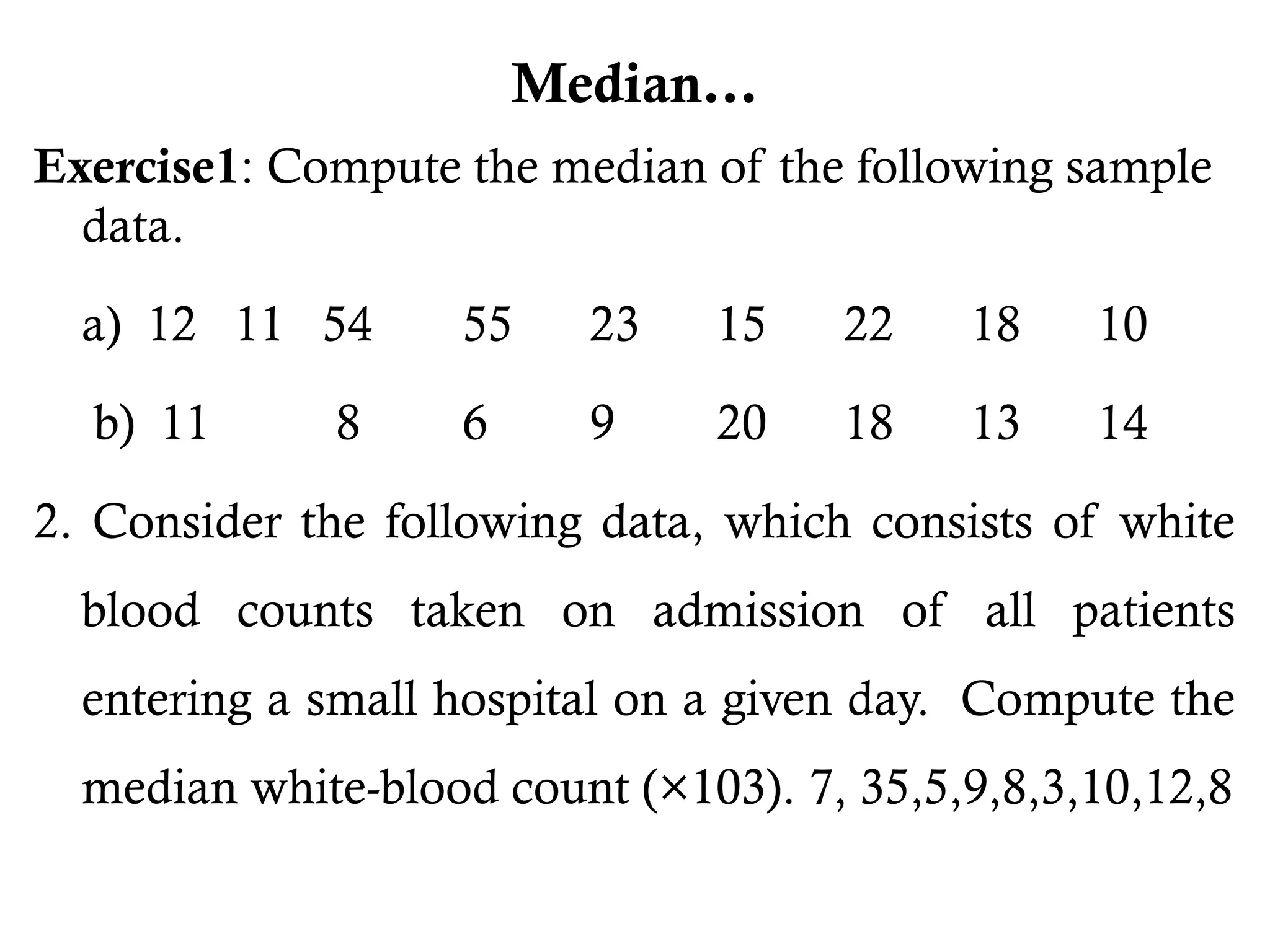
20. Median…
Exercise1: Compute the median of the following sample
data.
a) 12 11 54 55 23 15 22 18 10
b) 11 8 6 9 20 18 13 14
2. Consider the following data, which consists of white
blood counts taken on admission of all patients
entering a small hospital on a given day. Compute the
median white-blood count (×103). 7, 35,5,9,8,3,10,12,8

21. Median for Grouped data
~
x = L
n
2
F
f
W
m
c
m












Where:-
 Lm = lower true class boundary of the median class
 Fc = cumulative frequency of the class interval just above the
median class (median class=n/2)
 fm = absolute frequency of the median class
 W= class width (class with of the median class)
 n = total number of observations

22. Median…
Example 3: Consider the following grouped data on
the amount of time ( in hours) that 80 college students
devoted to leisure activities during a typical school
week. Time Frequency Cumulative feq
10-14 8 8
15-19 28 36
20-24 27 63
25-29 12 75
30-34 4 79
35-39 1 80
Total 80

23. Characteristics of median
1) It is an average of position
2) It is affected by the number of items rather than by extreme
values
Advantages
 It is easily calculated and is not much affected by extreme
values
 It is more typical of the series
 It may be located even when the data are incomplete, e.g, when
the class intervals are irregular and the final classes have open
ends

24. Characteristics of median…
Disadvantages
The median is not so well suited to algebraic
treatment as the arithmetic, geometric and harmonic
means
It is not so generally familiar as the arithmetic mean

25. 3. Mode
 is the value which occurs most frequently
 the mode may not exist, and even if it does, it may not be
unique
 it is the least useful (and least used) of the three
measures of central tendency
 When the distribution has only one vale with highest
frequency it is called Uni-modal
 If it has two values with equal and highest frequency it is
called Bi-modal
 Similarly, it is possible to have multi-modal frequency
Example: {1, 2, 2, 3, 3, 4, 4, 4, 5}
 The mode is 4, which is Uni-modal

26. Mode for grouped data
usually refer to the modal class interval
the modal class is the interval with the highest frequency
Mode = L+W × D1
D1+D2
Where:-
L= lower class limit of the modal class
D1=Excess of modal frequency over frequency of next lower class
D2=Excess of modal frequency over frequency of next higher class
W= size of the modal class interval

27. Mode for grouped data…
Example 1: Calculate the mode of the given data
 the modal class is 45-55, with a frequency of 31
 the lower class limit of the modal class is 45
 D1=31-29 =2
 D2= 31-5= 26
 W= 10
Mode= 45+ 10 × 31-29
31-29+ 31-5
= 45.7
CL 5-15 15-25 25-35 35-45 45-55 55-65 65-75
F 8 12 17 29 31 5 3

28. Mode for grouped data…
Example 1: Calculate the mode of the given data
 the modal class is____, with a frequency of ___
 the lower class limit of the modal class is ___
 D1=
 D2=
 W=
Mode=
CL 0-10 10-20 20-40 40-60 60-80 80-100
F 10 15 25 30 14 6

29. Characteristics of Mode
It is not affected by extreme values
It is the most typical value of the distribution
Advantages
 Since it is the most typical value it is the most
descriptive average
 Since the mode is usually an “actual value”, it indicates
the precise value of an important part of the series
Disadvantages
 It is not capable of mathematical treatment
 In a small number of items the mode may not exist

30. II. Measures of Variation/ Dispersion
While measures of central tendency are used to estimate
"centeral" value of a data set, measures of dispersion are
important for describing the spread of the data, or its
variation around a central value
Two distinct samples may have the same mean or median, but
completely different levels of variability, or vice versa
Set 1: 30, 40, 40, 50, 60, 60, 70 (Mean = 50)
Set 2: 48, 49, 49, 50, 50, 51, 53 (Mean = 50)

31. Measures of Variation/ Dispersion…
The objective of measuring this scatter or dispersion is to
obtain a single summary figure which adequately exhibits
whether the distribution is compact or spread out
 are important for describing the spread of the data or its
variation around a central value
Some of the commonly used measures of dispersion
(variation) are:
1. Range (R)
2. Interquartile range (IQR)
3. Variance (S2
)
4. Standard deviation (SD) and
5. Coefficient of variation (CV)

32. 1. Range
 the difference between the highest and smallest
observation in the data
 it is the crudest measure of dispersion
 it is a measure of absolute dispersion and
 cannot be usefully employed for comparing the
variability of two distributions expressed in different
units
Range = Xmax - Xmin
Where ,
Xmax = highest (maximum) value in the given distribution
Xmin = lowest (minimum) value in the given distribution

33. Characteristics of Range
 Since it is based upon two extreme cases in the entire
distribution, the range may be considerably changed if either
of the extreme cases happens to drop out, while the removal
of any other case would not affect it at all
 It wastes information for it takes no account of the entire data
 The extreme values may be unreliable; that is, they are the
most likely to be faulty
 Not suitable with regard to the mathematical treatment
required in driving the techniques of statistical inference

34. 2. Quantiles
 are another approach that addresses some of the
shortcomings of the range
 Of three types
i. Quartiles:- which divides a given set of data into four
equal parts
ii. Deciles:- which divides the given set of data into ten
equal parts
iii. Percentiles:- which divides the given set of data into
hundred equal parts

35. A. Quartiles
 is a measure of dispersion which divides the given set of
data into four equal parts
 it will have three quartile such as Q1,Q2, & Q3
the three quartiles Q1, Q2, and Q3 divide an ordered data set
into four equal parts
– About ¼ of the data falls on or below the first quartile
Q1
– About ½ of the data falls on or below the second
quartile Q2 (equivalent to median)
– About ¾ of the data falls on or below the third quartile
Q3

36. Quartiles…
In order to identify the Quartiles of a given dataset:
 Sort the values in increasing order
 Identify the Quartiles accordingly;
• Q1 = [(n+1)/4]th
• Q2 = [2(n+1)/4]th
• Q3 = [3(n+1)/4]th
The inter-quartile range is the difference between the third and the
first quartiles.
IQR = Q3 - Q1

37. A. First Quartile
 is called Q1
 is a lowest quartile
 it calculates the 25% of the given data
its meaning is 25% of the observation are below Q1 but
75% of the observation is above Q1 .
it is calculated as:-
Q1 = 1 n +1 th
observation
4
=0.25(n+1)th
observation

38. B. Second Quartile
 is called Q2
 is a lower or the middle quartile
 it calculates 50% of the given data
 its meaning 50% of observations are below Q2 and
50% are above Q2
 is called median
it is calculated as:-
Q2 = 2 n +1 th
observation
4
=0.5(n+1)th
observation

39. C. Third Quartile
 is called Q3
 it is a upper/highest quartile
 it calculates the 75% of the given data
 its meaning 75% are below Q3 and 25% are above
Q3
 it is calculated as:-
Q3 = 3 n +1 th
observation
4
=0.75(n+1)th
observation

40. Examples:-
1. Let’s assume the following dataset presents the age of 8 factory
workers. {18, 21, 23, 24, 24, 32, 42, 59}
• Identify the first and the third quartiles
Solution:
• First make sure that the data is sorted in increasing order
• Q1 is the {0.25 (n+1)}th
observation
 {0.25 (8+1)}th
observation
 {0.25 (9)}th
observation
 {2.25}th
observation

41. Examples…
• i.e. the Q1 is a quarter distance between 21 and 23 this can be
interpolated as:
 21 + (23-21)0.25 = 21.5
• The interpretation is one forth of the observations are below or equal
to the value 21.5
• Q3 is the {0.75(n+1)} th
observation
 {6.75}th
observation
 32 + (42-32)0.75 = 39.5
• The interpretation is three forth of the observations are below or equal
to the value 39.5

42. Examples…
2. Calculate Q1 ,Q2 ,Q3 and IQR, and give interpretation
for the following datasets.
18, 29, 14, 42, 31, 23, 44, 32, 54

43. 2. Percentiles( Reading assignment)
 Divides the given set of observations into 100 equal parts
 Each group represents 1% of the data set
 There are 99 percentiles termed P1 through P99
 The 25th
percentile is the first quartile (P25=Q1)
 The 50th
percentile is the median (P50 = Median)
 The 75th
percentile is the third quartile (P75=Q3)
 The interpretation of Percentiles is as follows:
 1% of the data falls on or below P1
 2% of the data falls on or below P2

44. Percentiles…
Pth
percentile is defined as:-
i. (K+1)th
observation , if np/100 is not an integer.
K is the largest integer below np/100.
ii. (np/100) th
obser+( np/100+1)th
obser,
2
if np/100 is an integer.

45. Examples:-
1. Calculate P25% ,P50% ,P75% P80%, and P70% give interpretation
for the following datasets.
18, 29, 14, 42, 31, 23, 44, 32, 54

46. 2. Variance and standard deviation
 measure how far an average score deviate from the mean
 thus variance is as the sum of the square of the deviation
of each observation from the mean divided by total
number of observation minus 1
 the variance represents squared units and, therefore, is
not an appropriate measure of dispersion when we wish
to express this concept in terms of original units
 to obtain a measure of dispersion in original units,
we merely take the square root of the
variance( standard deviation)

47. Variance and standard deviation…
 It is positive square root of the variance
 Standard deviation is the most commonly used
measure of dispersion
 Standard deviation is the average deviation from the
mean (expressed in the original units)
 Standard deviation is measure of absolute deviation

48. Variance and standard deviation…
 the formulas for sample and population variance are
given as follows:
Sample variance Population variance
 occasionally, the abbreviations SD for standard deviation
and Var (S2
) for variance are used
1
)
(
1
2
2





n
x
x
S
n
i
i
n
x
n
i
i



 1
2
2
)
(


49. Variance and standard deviation…
 standard deviation for grouped data is calculated as:
Where
S = standard deviation
mi = class mark
x = mean
fi = frequency
n = number of observation
1
)
(
1
1
2







n
f
n
f
x
m
S
i
i
i
i
i

50. Why squared?
Why square differences between data values and mean?
Gives positive values
Gives more weight to larger differences
Has desirable statistical properties
Why n - 1 for sample variance?
Dividing by n underestimates population variance
Dividing by n-1 gives unbiased estimate of population
variance

51. Variance and standard deviation…
Example. Find the standard deviation of the numbers 12, 6,
7, 3, 15, 10 ,18, 5.
 Solution: x = (12+6+7+3+15+10+18+5) /8= 9.5
 The variance is
s2
= [(12-9.5)2
+…+ (5-9.5)2
]/ (8-1) = 5.21
The standard deviation is s = √5.21 =2.28

52. Variance and standard deviation…
Advantages:
they accommodate further mathematical applications (SD)
they are calculated from the whole observations
Disadvantages:
they must always be understood in the context of the mean
of the data
thus it is difficult to compare the standard
deviation/variance of two datasets measured in two
different units

53. Example
1.Consider the data on the weight of 10 new born children
at Zewiditu hospital within a month: 2.51, 3.01, 3.25,
2.02,1.98, 2.33, 2.33, 2.98, 2.88, 2.43.
Calculate
a) Range (1.27)
b) Variance (0.198)
c) Standard deviation(0.44)

54. 3. Coefficient of variation (CV)
 measure of relative variation/dispersion
 use to compare variation of distributions with different
units relative to their means
 it is also sometimes called coefficient of dispersion
 this is a good way to compare measures of dispersion
between different samples whose values don’t
necessarily have the same magnitude (or, for that matter,
the same units!)

55. Coefficient of variation…
%
100
x
x
S
CV 
the standard formulation of the CV is the ratio of the
standard deviation to the mean of a give data
the coefficient of variation is a dimensionless number
So when comparing between data sets with different units
one should use CV instead of SD
the CV is useful in comparing the variability of several
different samples, each with different arithmetic mean as
higher variability is expected when the mean increases
 CV is also important to compare reproducibility of
variables

56. Coefficient of variation…
Example1:- One patient’s blood pressure, measured
daily over several weeks, averaged 182 with a
standard deviation of 12.6, while that of another
patient averaged 124 with a standard deviation of
9.4. Which patient’s blood pressure is relatively more
variable?

57. Given s1=12.6 s2= 9.4 x1=182 x2= 124
923
.
6
%
100
182
6
.
12
1 
 x
CV
58
.
7
%
100
124
4
.
9
2 
 x
CV
blood pressure of the second patient is relatively more
variable

58. Example 2
Suppose two samples of male individuals yield the following
results.
A comparison of the standard deviations might lead one to
conclude that the two samples posses’ equal variability
Sample 1 Sample2
Age 25 years 11 years
Mean weight 145 pounds 80 pounds
Standard deviation 10 pounds 10 pounds
We wish to know which is more variable, the weights of the 25-
year- olds or the weights of the 11-year-olds

59.  If we compute the coefficients of variation, however,
have for the 25-year-olds
C.V=10/145(100) =6.9
And for the 11-year-olds
C.V=10/80(100) =12.5
If we compare these results we get quite a different
impression

60. Example
1. The following table shows the number of hours 45
hospital patients slept following administration of a
certain anesthetic medication (10pts)
7 10 12 4 8 7 3 8 5
12 11 3 8 1 1 13 10 4
4 5 5 8 7 7 3 2 3
8 13 1 7 17 3 4 5 5
3 1 17 10 4 7 7 11 8

61. After grouping the above data in to frequency
distribution table compute the following:-
a. Mean
b. Median
c. Mode
d. Variance
e. Standard deviation
f. Coefficient of variation

62. Thank You!!!!!!