The document discusses probabilistic analysis in the context of algorithm complexity, particularly focusing on the hiring problem and insertion sort. It presents the concept of modeling randomness through indicator random variables and the advantages of enforcing uniform distribution assumptions to improve average-case performance. The document also introduces algorithms for randomization and their implications for hiring and sorting processes.

1. Probabilistic Analysis
Andres Mendez-Vazquez
January 21, 2016
Contents
1 Introduction 2
2 The Hiring Problem 2
3 Did you notice the following? 3
4 The Indicator Random Variables 3
5 Analyzing Random Hiring 5
6 Enforcing the Uniform Assumption 6
6.1 Lemma for Permute By Sorting . . . . . . . . . . . . . . . . . . . 7
6.2 Lemma for Randomize in Place . . . . . . . . . . . . . . . . . . . 8
7 Application of Probabilistic Analysis: Insertion Sort 9
1

2. 1 Introduction
Do you remember the words the “average case”? Actually, these words have a
deeper meaning with respect to what we call a probability and its associated
distribution. Thus, using probability is possible to model the inherent stochastic
event branch structure while running an specific algorithm in an input.
Once you realized the advantages of using probability for complexity anal-
ysis, it is clear that you require to know the distribution where your inputs
operate. Oh!!! Looks fancy, far from it because you already have a course of
probability making easy to understand the following way of modeling branch
randomness over an specific input. Not only that, there are algorithms where
given the “average input,” they behave better than in the worst case. Where
these “average inputs” are inputs randomized using a uniform distribution [2, 1].
Therefore, if we want to obtain the best behavior of those algorithms, we need
to prove that the randomization produce inputs coming from a uniform distri-
bution.
Therefore, to exemplify all these strategies we will start looking at the
stochasticity of the hiring problem [3].
2 The Hiring Problem
The hiring problem exemplifies the classic problem of scanning trough an input
and taking decision on each section of that input. The problem is defined the
following way.
Definition 1. A company needs to hire a new office assistant from a batch
{x1, x2, ..., xn} of possible candidates provided by an employment agency. The
company has the following constraints about the hiring process:
1. We need to interview all the candidates.
2. The job position is never empty.
While looking at this definition of the hiring problem, we notice the following
constraints or restrictions:
• We might hire m of them.
• The cost constraints for each of the possible events are:
– Cost of interviewing: ci per candidate.
– Cost of hiring: ch per candidate.
In addition, we have that ch > ci i.e. the cost of hiring is larger than the cost
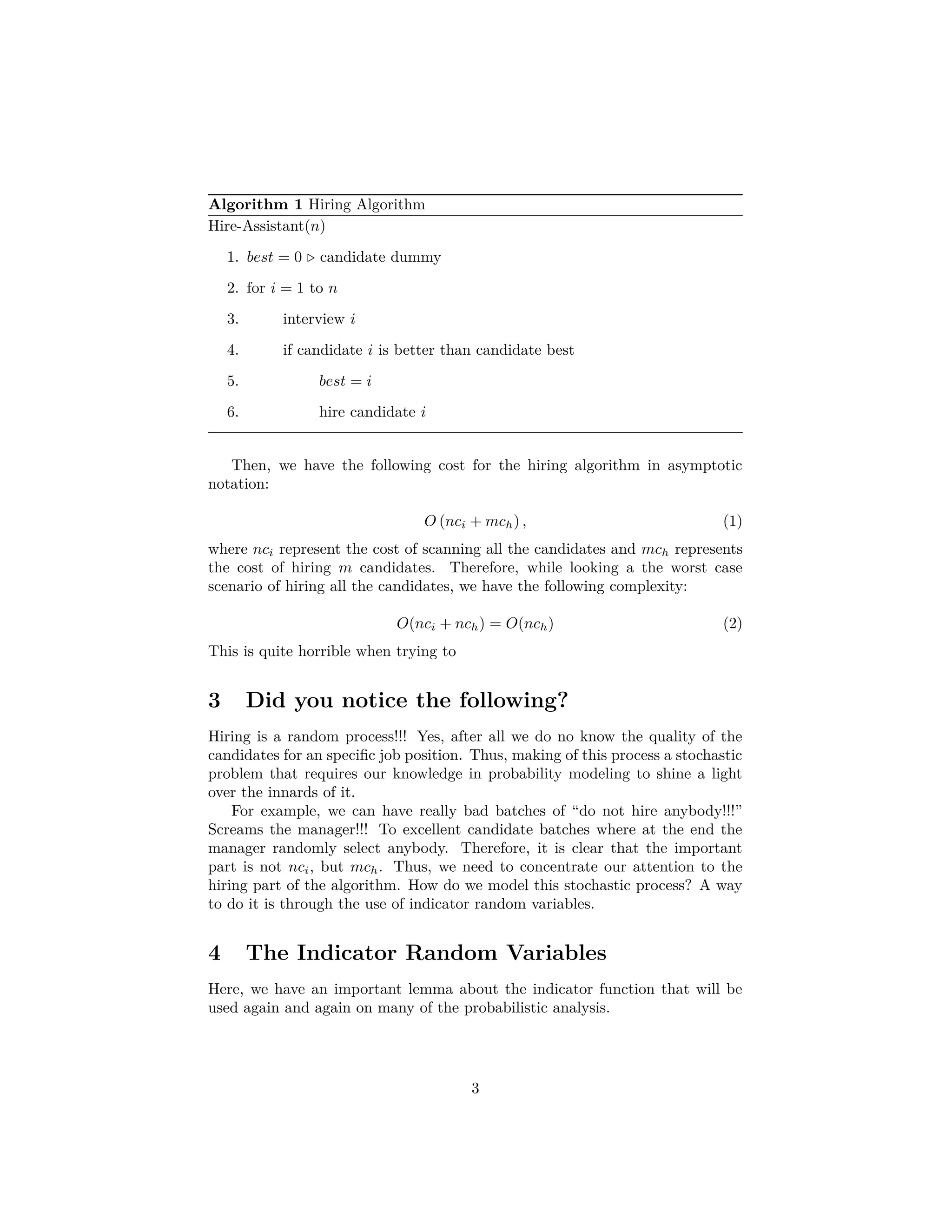
of doing an interview. Thus, we have the following algorithm (Algorithm 1) for
the hiring process.
2

3. Algorithm 1 Hiring Algorithm
Hire-Assistant(n)
1. best = 0 candidate dummy
2. for i = 1 to n
3. interview i
4. if candidate i is better than candidate best
5. best = i
6. hire candidate i
Then, we have the following cost for the hiring algorithm in asymptotic
notation:
O (nci + mch) , (1)
where nci represent the cost of scanning all the candidates and mch represents
the cost of hiring m candidates. Therefore, while looking a the worst case
scenario of hiring all the candidates, we have the following complexity:
O(nci + nch) = O(nch) (2)
This is quite horrible when trying to
3 Did you notice the following?
Hiring is a random process!!! Yes, after all we do no know the quality of the
candidates for an specific job position. Thus, making of this process a stochastic
problem that requires our knowledge in probability modeling to shine a light
over the innards of it.
For example, we can have really bad batches of “do not hire anybody!!!”
Screams the manager!!! To excellent candidate batches where at the end the
manager randomly select anybody. Therefore, it is clear that the important
part is not nci, but mch. Thus, we need to concentrate our attention to the
hiring part of the algorithm. How do we model this stochastic process? A way
to do it is through the use of indicator random variables.
4 The Indicator Random Variables
Here, we have an important lemma about the indicator function that will be
used again and again on many of the probabilistic analysis.
3

4. Lemma Given a sample space S and an event A in the sample space S, let
XA = I {A}. Then, E (XA) = Pr {A}.
Proof:
Simply look at this
E (XA) = E (I {A}) = 1 × Pr {A} + 0 × Pr A = Pr {A} (3)
Thus, it is possible to use the previous equivalence to solve many problems
by decomposing many complex events in a probability space by using a simple
formula.
Example 2. For example, given a coin being flipped n times. W can define the
following random variable X =The number of heads in n flips of a coin. This
can be decomposed into a sequence of random variables Xi = I{At ith flip you
get a head} by making the simple observation:
X = X1 + X2 + ... + Xn =
n
i=1
Xi (4)
Therefore, taking the expected value in both sides of the equation, we have that
E [X] = E
n
i=1
Xi =
n
i=1
E [Xi] =
n
i=1
1
2
=
n
2
(5)
Another example is using a Bernoulli distribution to guess how many nuclear
missiles will hit their targets.
Example 3. Given that the probability of hitting a target by nuclear missile
is p. Now, you launch n of them to it, thus ¿How many of them will hit the
target? First every launch is a Bernoulli trial. Now, given that Xi = I{The ith
launch hits the target}. The total number of successes is
X = X1 + X2 + ... + Xn (6)
Then, again using the Bernoulli and expected value:
E [X] = E [X1 + X2 + ... + Xn] (7)
Thus, by the linearity of the expectation E [X] = E [X1] + E [X2] + ... + E [Xn]
where E [Xi] = P (Ai) = p. Finally,
E [X] =
n
i=1
E [Xi] =
n
i=1
p = np.
4

5. 5 Analyzing Random Hiring
Now, we analyze the hiring from the randomized point of view. For this, we first
assume that the candidates are interviewed in a random way using a uniform
distribution which is called the Uniform Assumption. This allows to assume
that any of the candidates, when we have i of them, could be hired. This can
be represented by the following random indicator variable:
Xi = I {Candidate i is hired} =
1 if candidate i is hired
0 if candidate i is not hired
(8)
Thus, we have the following probability for the event “Candidate i is hired”:
Pr {Candidate i is hired} =
1
i
. (9)
This can only happen if candidate i is better than the previous i−1 candidates.
Finally, we have an “average case”:
E [Xi] = Pr {Cantidate i is hired} =
1
i
. (10)
Now, we can generate a new random variable that represents:
X = The total number of hirings, (11)
which can be decomposed in a sequence of simpler random variables:
X = X1 + X2 + ... + Xn (12)
Now, if we apply the expected value to both sides of the equation, we have
E [X] =E
n
i=1
Xi =
n
i=1
E [X] (Linearity of the Expected Value)
=
n
i=1
1
i
= 1 +
n
i=2
1
i
≤1 +
ˆ n
1
1
i
di (Decreasing Function)
=1 + ln n,
Therefore, the expected value or average case has the following complexity:
E [X] = ln n + O (1) (13)
Then, the final cost of hiring is O (ch ln n) . Actually this proof of the complexity
O(ch log n) is the same once we notice that the permutation of the elements is
giving us the same situation as in the hiring when the input order (The order
of interviewing) is drawn from a uniform distribution.
Therefore, given the differences between worst case hiring and randomized
hiring is quite extreme, it could be a good idea to enforce the uniform assumption
to get the better expected complexity.
5

6. 6 Enforcing the Uniform Assumption
Imagine now that
• The employment agency sends us a list of all n candidates in advance.
• On each day, we randomly choose a candidate from the list to interview.
• Instead of relaying on the candidate being presented to us in a random
order, we take control of the process and enforce a random order.
This is giving us the idea of a randomized algorithm where
• An algorithm is randomized if its behavior is determined in part by
values produced by a random-number generator.
• A random-number generator [4] is implemented by a pseudorandom-
number generator, which is a deterministic method returning numbers
that “look” random and can pass certain statistical tests.
An example of a randomized algorithm version of hiring can be seen in (Algo-
rithm 2).
Algorithm 2 Hiring Algorithm
Randomized-Hire-Assistant(n)
1. Randomly Permute the list of candidates
2. best ← 0 candidate dummy
3. for i = 1 to n
4. interview i
5. if candidate i is better than candidate best
6. best ← i
7. hire candidate i
We have a small problem in the line on where the algorithms “Randomly
Permute the list of candidates.” For this, we are required to have algorithms
that enforce the uniform assumption on that instruction. The algorithms that
we are going to see in this course are:
• Permute By Sorting (Algorithm 3).
• Randomize in Place (Algorithm ).
Each of them uses a lemma to prove that they enforce the uniform assump-
tion in an input.
6

7. Algorithm 3 Permute By Sorting Algorithm
Permute-By-Sorting(A)
1. n = lenght[A]
2. for i = 1 to n
3. do P[i] = RANDOM 1, n3
4. sort A, using P as sort keys
5. return A
Algorithm 4 Randomize in Place Algorithm
Randomize-In-Place(A)
1. n = lenght[A]
2. for i = 1 to n
3. do swap A[i] ←→ A[RANDOM(i, n)]
6.1 Lemma for Permute By Sorting
In this section, we prove the fact that a randomization based in permutation
works if we can trust in our pseudo-random generator. Nevertheless, for a deeper
study on these random generators, we recommend to take a look at chapter 3
volume 2 of Donald Kunth “The Art of Computer Programming” [4].
Lemma 5.4
Procedure Permute-by-sorting produces a uniform random permutation
of the input, assuming that all probabilities are distinct.
Proof:
Case I
Assume A[i] receives the ith smallest priority. Let Ei be the event that
element A[i] receives the ith
smallest probability. Therefore, we wish to
compute the event the probability of event E1 ∩ E2 ∩ ... ∩ En, and given
that we haven! possible permutations of the ranking, we want to be sure
that the P(E1 ∩ E2 ∩ ... ∩ En) = 1
n! . This event is the most naive one,
it means that A[1]is the 1st element, A[2] is the 2nd element and so on.
Then, it is simply a case of using the chain rule:
P(E1, E2, ..., En) = P(En|E1, ..., En−1)P(En−1|E1, ..., En−2)...
P(E2|E1)P(E1)
(14)
7

8. First imagine that you have n possible positions at your array and you
need to fill them. Now look at this:
• At E1 you have n different elements to put at position one or P(E1) =
1
n .
• At E2 you have n − 1 different elements to put at position two or
P(E2|E1) = 1
n−1 .
• etc.
Therefore, P(E1, E, ..., En) = 1 × 1
2 × 1
3 × ... × 1
n = 1
n! .
Case II
In the general case, we have that we can use for any permutation σ =
σ(1), σ(2), ..., σ(n) of the set {1, 2, ..., n}. Let us to assign rank ri to the
element A[i]. Then, if we define Ei as the event in which element A[i]
receives the σ(i)th
smallest priority such that ri = σ(i), we have the same
proof.
QED
6.2 Lemma for Randomize in Place
Now, we prove the the randomization in place can enforce the uniform assump-
tion.
Lemma 5.5
Procedure RANDOMIZE-IN-PLACE computes a uniform random permu-
tation.
Proof:
We use the following loop invariant, before entering lines 2-3 the array A[1, ..., i−
1] contains a (i − 1)-permutation with probability (n−i+1)!
n! .
Initialization. We have an empty array A[1, ..., 0] and i = 1, then P(A[1, ..., 0]) =
(n−i+1)!
n! = n!
n! = 1. This is because of vacuity.
Maintenance. Then, by induction, we have that the array A[1, ..., i − 1] con-
tains (i − 1)-permutation with probability (n−i+1)!
n! . Now, consider the
i-permutation contain the elements x1, x2, ..., xi = x1, x2, .., xi−1 ◦ xi.
Then, E1denotes the event for the (i − 1)-permutation with P(E1) =
(n−i+1)!
n! , and E2 denotes putting element xi at position A[i]. Therefore,
we have that P(E2 ∩ E1) = P(E2|E1)P(E1) = 1
n−i+1 × (n−i+1)!
n! = (n−i)!
n! .
Termination. Now with i = n + 1 we have that the array A[1, ..., n] contains
a n−permutation with probability (n−n+1)!
n! = 1
n! .
8

9. 7 Application of Probabilistic Analysis: Inser-
tion Sort
From chapter 1, it was possible to see that the total number of steps done by
the insertion sort is
n + I, (15)
where I is a random variable that count the total number of possible inversions.
Here, the event of an inversion at positions i and j of an array A can be described
by an indicator random variable:
Iij = I {if i < j A [i] > A [j]} . (16)
Then, we have that
I =
n
i=1
n
j=1,i=j
Iij. (17)
Now, we get the final formulation of the number of steps for insertion sort as
n + I = n +
n
i=1
n
j=1,i=j
Iij. (18)
Finally, we can apply the the expected value to both sides of the equation
E [n + I] = E

n +
n
i=1
n
j=1,i=j
Iij

 , (19)
and because the linearity of the expected value (n is a constant), we have that
E [n + I] =n + E [I]
=n + E


n
i=1
n
j=1,i=j
Iij


=n +
n
i=1
n
j=1,i=j
E [Iij] .
Now, we have that, by assuming the uniform assumption,
E [Iij] =
1
2
. (20)
Finally,
E [n + I] = n +
n
i=1
n
j=1,i=j
1
2
= n +
1
2
n
i=1
n
j=1,i=j
1 = n +
n (n − 1)
2
, (21)
because
n
i=1
n
j=1,i=j 1 counts the number of different pair that you can count
with n elements. Thus, the complexity of insertion sort for the average case is
O n +
n (n − 1)
2
= O
n
2
+
n2
2
= O n2
. (22)
9

10. References
[1] R.B. Ash. Basic Probability Theory. Dover Books on Mathematics Series.
Dover Publications, Incorporated, 2012.
[2] George Casella and Roger L. Berger. Statistical Inference. Pacific Grove:
Duxbury Press, second edition, 2002.
[3] Thomas H. Cormen, Charles E. Leiserson, Ronald L. Rivest, and Clifford
Stein. Introduction to Algorithms, Third Edition. The MIT Press, 3rd edi-
tion, 2009.
[4] Donald E. Knuth. The Art of Computer Programming, Volume 2 (3rd Ed.):
Seminumerical Algorithms - Chapter 3 - Random Numbers. Addison-Wesley
Longman Publishing Co., Inc., Boston, MA, USA, 1997.
10