Thesis

1
ABSTRACT
REPAIR TIME MODEL FOR DIFFERENT BUILDING SIZES
CONSIDERING THE EARTHQUAKE HAZARD
By
Dong Y. Yoo
August 2016
Recent earthquakes devastated lives and destroyed a great stock of buildings. As
a result, the earthquake-impacted regions incurred huge business and operation
interruption losses. To minimize the business interruption losses through Performance-
Based Seismic Design, there is an obvious need for a validated downtime model that
would cover a large spectrum of building sizes and types. Building downtime consists of
securing finances, mobilizing contractors, engineers and supplies, and the time to perform
the actual repair, i.e., repair time. This study focuses on developing a model to
characterize the repair time contribution to the downtime as an extension to FEMA P-58
Loss Assessment Methodology. The proposed repair time model utilizes the Critical Path
Method for repair scheduling and realistic labor allocations that are based on the amount
and severity of building damage. The model is validated on a significant sample of data
collected through case studies from previous earthquakes, interviews with contractors,
engineers, and inspectors. The proposed model also has a capability of scheduling
resources to meet resource limitations that can either come from labor congestions or

2
from a surge in demands following a disaster. The proposed resource scheduling method
provides an efficient way of reducing the number of workers during labor congestions
while minimizing its effect on the project duration. The final outcome is a realistic
estimation of repair time associated with an earthquake.

REPAIR TIME MODEL FOR DIFFERENT BUILDING SIZES
CONSIDERING THE EARTHQUAKE HAZARD
A THESIS
Presented to the Department of Civil Engineering and
Construction Engineering Management
California State University, Long Beach
In Partial Fulfillment
of the Requirements for the Degree
Master of Science in Civil Engineering
Committee Members:
Vesna Terzic, Ph.D. (Chair)
Lisa Star, Ph.D.
Luis G. Arboleda-Monsalve, Ph.D.
College Designee:
Antonella Sciortino, Ph.D.
By Dong Y. Yoo
B.S., 2013, University of California, San Diego
August 2016

All rights reserved
INFORMATION TO ALL USERS
The quality of this reproduction is dependent upon the quality of the copy submitted.
In the unlikely event that the author did not send a complete manuscript
and there are missing pages, these will be noted. Also, if material had to be removed,
a note will indicate the deletion.
All rights reserved.
This work is protected against unauthorized copying under Title 17, United States Code
Microform Edition © ProQuest LLC.
ProQuest LLC.
789 East Eisenhower Parkway
P.O. Box 1346
Ann Arbor, MI 48106 - 1346
ProQuest 10142981
Published by ProQuest LLC (2016). Copyright of the Dissertation is held by the Author.
ProQuest Number: 10142981

Copyright 2016
Dong Y. Yoo
ALL RIGHTS RESERVED

iii
ACKNOWLEDGEMENTS
Dr. Vesna Terzic and I acknowledge financial support for this work from the
Pacific Earthquake Engineering Research Center under the project 2002-NCEEVT. We
are grateful for the Applied Technology Council providing the latest release of the PACT
software application. The conclusions, observations, and findings presented herein are
those of the authors and not necessarily those of the sponsors.
I sincerely thank Dr. Vesna Terzic for her guidance and encouragement during the
course of our research studies. Her patience and dedication as a professor and an advisor
had a profound impact in my structural engineering career. I wish to express my sincere
gratitude to Bob Berenguer and Gene Calkin of KPRS Construction, John F. Rochford,
Fred Wallitsch and Richard Cavecche of Snyder Langston, Jesse Karns of Mitek
Industries, and Lance Kenyon of MHP Structural Engineers for their efforts and
involvement in our research studies. Their contributions were invaluable in finishing my
thesis. Lastly, I would like to thank our undergraduate research assistants, Daniel
Saldana and Bryan Simental for their contributions.
Finally, I wish to express my deepest gratitude to my caring, loving, and
supportive wife, Iris. Her encouragement and support have helped me get to where I am
today. Lastly, I would like to thank my parents for all of their supports and express my
sincere gratitude for my family.

iv
TABLE OF CONTENTS
Page
ACKNOWLEDGEMENTS......................................................................................... iii
LIST OF TABLES....................................................................................................... vi
LIST OF FIGURES ..................................................................................................... vii
CHAPTER
1. INTRODUCTION ............................................................................................ 1
1.1 Organization of Report ........................................................................ 4
2. REVIEW OF EXISTING REPAIR TIME MODELS...................................... 6
2.1 Optimal Strategy for Business Recovery after Earthquakes................ 6
2.2 Assembly-Based Vulnerability (ABV) Methodology ......................... 7
2.3 FEMA P-58: Repair Time Estimation ............................................... 10
2.4 Arup and Arup's REDi™ Rating System: Repair Time Model.......... 15
2.5 Conclusion ........................................................................................... 19
3. REPAIR SCHEDULING METHODOLOGY.................................................. 20
3.1 Existing Scheduling Techniques.......................................................... 21
3.1.1 Critical Path Method............................................................. 21
3.1.2 Line of Balance Method........................................................ 22
3.2 Differences Between New Construction and Repair Work ................. 24
3.3 Repair Scheduling Method .................................................................. 25
3.3.1 Terms and Definitions........................................................... 26
3.3.2 Initial Parameters .................................................................. 27
3.3.3 Repair Scheduling Method ................................................... 29
3.4 Example of Repair Scheduling ............................................................ 34
3.4.1 Initial Parameters .................................................................. 34
3.4.2 Repair Time Duration and Resources................................... 37
3.4.3 Repair Time Calculations Based on CPM ............................ 38
3.4.4 Results................................................................................... 42

v
CHAPTER Page
3.5 Conclusion ........................................................................................... 43
4. RESOURCE SCHEDULING METHOD......................................................... 44
4.1 Existing Resource Scheduling Methodologies .................................... 46
4.1.1 Overview of Difference Resource Modeling and Graphing
Techniques............................................................................. 46
4.1.2 Packing Method for Resource Leveling (PACK)................. 50
4.1.3 Modified Minimum Moment Approach in Resource ..........
Leveling ................................................................................ 51
4.2 New Resource Scheduling Method...................................................... 54
4.3 Example in Resource Scheduling ........................................................ 56
4.4 Conclusion ........................................................................................... 63
5. DATA COLLECTION ON POST-EARTHQUAKE REPAIR OF
BUILDINGS.............................................................................................. 64
5.1 Interview Questions and Answers ....................................................... 64
5.2 Conclusion ........................................................................................... 70
6. CASE STUDIES OF 3 AND 12-STORY BUILDINGS .................................. 72
6.1 Case Study of a 3-Story Building ........................................................ 72
6.1.1 Repair and Resource Scheduling .......................................... 74
6.1.2 Results Using the New Repair Time Model ......................... 78
6.2 Case Study of a 12-Story Building ...................................................... 100
6.2.1 Repair and Resource Scheduling .......................................... 102
6.2.2 Results Using the New Repair Time Model ......................... 102
7. CONCLUSION AND RECOMMENDATIONS ............................................. 126
REFERENCES ............................................................................................................ 130

vi
LIST OF TABLES
TABLE Page
1. Component Subgroups Described in Arup's REDi™....................................... 17
2. Sample Worker Allocation ............................................................................... 31
3. Initial Parameters of All Activities Listed in the Example............................... 36
4. Arbitrary Repair Duration and Resources of Each Activity............................. 37
5. Repair Duration, Resources (Number of Workers) and Final Durations.......... 41
6. Start Date, Finish Date and Free Float of All Activities................................... 41
7. Repair Time Chart After Resource Scheduling ................................................ 62
8. Realistic Distributions of Workers Based on the Interviews Using Average
Damage State (ADS) and Number of Damaged Units (NDU).................. 68
9. Initial Parameters of Repair Time Model of 3-Story Building......................... 77

vii
LIST OF FIGURES
FIGURE Page
1. Functionality function of a building system after an earthquake...................... 3
2. Median repair time of a 12-story building in parallel schedule and serial
schedule...................................................................................................... 14
3. Filtering of data in REDi™ procedure.............................................................. 19
4. An example of the line of balance technique.................................................... 23
5. Flowchart of the proposed repair scheduling methodology.............................. 33
6. Repair schedule of a generic example .............................................................. 35
7. Activity-on-node diagram of a generic example .............................................. 36
8. Repair schedule displayed using Gantt chart of a generic 3-story building ..... 42
9. Example of a histogram in an aggregation method.. ........................................ 47
10. Example of a histogram in an accumulation method...................................... 48
11. Flowchart of the proposed resource scheduling methodology ....................... 57
12. Repair schedule before resource scheduling and activity stretching ............... 59
13. Resource histogram before the proposed resource scheduling method........... 59
14. Repair schedule after resource scheduling and activity stretching .................. 61
15. Resource histogram after the proposed resource scheduling method.............. 61
16. Special moment resisting frame configuration (Frames located only on
perimeters of the building)......................................................................... 73

viii
FIGURE Page
17. Median inter story drift ratios and median floor accelerations of the 3-story
building for fault parallel (FP) and fault normal (FN) directions of
shaking for three hazard levels .................................................................. 74
18. Flowchart of a realistic repair schedule of a 3-story SMRF building ............. 75
19. Activity-on-node diagram of a realistic repair schedule of a 3-story SMRF .
building ..................................................................................................... 76
20. Probability distribution curve at the 50% in 50 year hazard level................... 80
21. Repair schedule at the median and the 50% in 50 year hazard level............... 81
22. Resource histogram at the median and the 50% in 50 year hazard level......... 81
23. Repair schedule at the 90% CL and the 50% in 50 year hazard level ............. 82
24. Resource histogram at the 90% CL and the 50% in 50 year hazard level....... 82
25. Comparison of total repair times with and without resource scheduling at
the 50% in 50 year hazard level (Intensity 1) ............................................ 83
26. Probability distribution curve at the 10% in 50 year hazard level................... 84
27. Repair schedule at the median and the 10% in 50 year hazard level............... 87
28. Resource histogram at the median and the 10% in 50 year hazard level......... 87
29. Repair schedule at the 90% CL and the 10% in 50 year hazard level ............. 88
30. Resource histogram at the 90% CL and the 10% in 50 year hazard level....... 88
31. Comparison of total repair times with and without stretching (resource
leveling) included in the repair time model at the 10% in 50 year hazard
level (Intensity 2)....................................................................................... 89
32. Probability distribution curve at the 2% in 50 year hazard level..................... 90
33. Repair schedule at the median and the 2% in 50 year hazard level................. 91
34. Resource histogram at the median and the 2% in 50 year hazard level........... 91

ix
FIGURE Page
35. Repair schedule at the 90% CL and the 2% in 50 year hazard level ............... 92
36. Resource histogram at the 90% CL and the 2% in 50 year hazard level ......... 92
37. Comparison of total repair times with and without stretching (resource
leveling) included in the repair time model at the 2% in 50 year hazard
level (Intensity 3)....................................................................................... 93
38. Repair schedule of realization #494 before resource scheduling..................... 96
39. Resource histogram of realization #494 before resource scheduling .............. 96
40. Repair schedule of realization #494 after resource scheduling ....................... 97
41. Resource histogram of realization #494 after resource scheduling ................. 97
42. Repair schedule of realization #10 before resource scheduling....................... 98
43. Resource histogram of realization #10 before resource scheduling ................ 98
44. Repair schedule of realization #10 after resource scheduling ......................... 99
45. Resource histogram of realization #10 after resource scheduling ................... 99
46. Median story drift ratios and median floor accelerations of the 12-story
SMRF at the design based earthquake....................................................... 101
47. Probability distribution curve at 67% of MCE design based earthquake ........ 104
48. Repair schedule at the median and design based earthquake .......................... 107
49. Resource histogram at the median and design based earthquake .................... 108
50. Resource histogram at the median and design based earthquake .................... 109
51. Repair schedule at the 90% CL and design based earthquake......................... 110
52. Resource histogram at the 90% CL and design based earthquake................... 111
53. Resource histogram at the 90% CL and design based earthquake................... 112

x
FIGURE Page
54. Comparison of total repair time with and without stretching (resource
leveling) at 67% of MCE ........................................................................... 113

1
CHAPTER 1
INTRODUCTION
Earthquakes in the past have demonstrated that they not only destroy buildings
and take away human lives, but also create enormous financial burdens to building
owners as a result of business and operational interruption losses. In 2010, a magnitude
8.8 earthquake in Chile demonstrated the crippling effects that nonstructural damage can
have on a city (Miranda et al. 2012). Buildings with only minor structural damage
sustained significant nonstructural damage and the widespread of nonstructural damage
caused building closures, which resulted in significant economic losses and major
disruption to Chilean society. In 2008, Toyoda presented a study that compared direct
and indirect losses from Kobe earthquake in 1995. Toyoda found that the indirect losses
in the commercial sector were twice greater than the direct losses in the same sector and
found that the lost product or income in terms of estimated indirect losses continued to
arise for longer than 10 years. His research showed that the total sum of indirect losses
during the period of 1994 and 2005 was about 14.0 trillion yen, which is about 124.6
billion US dollars (Toyoda 2008). To mitigate the earthquake-induced losses and
improve community resilience, building components essential for post-earthquake
functionality are to be protected through a better building design.
The Performance Based Earthquake Evaluation (PBEE) methodology, described
by Miranda and Aslani (2003), provides a probabilistic assessment framework to quantify

2
building’s performance considering performance metrics meaningful to decision makers,
stakeholders, and insurers (e.g., repair cost, downtime, return on investment).
Application of this methodology requires characterization of seismic hazard for a location
of interest, reliable numerical models of a soil-foundation-structure system,
characterization of damage states using fragility curves, and estimation of
losses/consequences using consequence functions. The PBEE methodology has been
recently adopted for general use through Federal Emergency Management Agency
[FEMA] P-58 initiative (FEMA 2012a; FEMA 2012b) by developing a comprehensive
library of peer-reviewed fragility curves and associated consequence functions
considering more than 700 structural and nonstructural building components, using
standard methods (Porter et al. 2001) and published data. Although the methodology
represents a step forward towards resilient design, there is a lack of appropriate downtime
and recovery models that are essential for measuring buildings resilience.
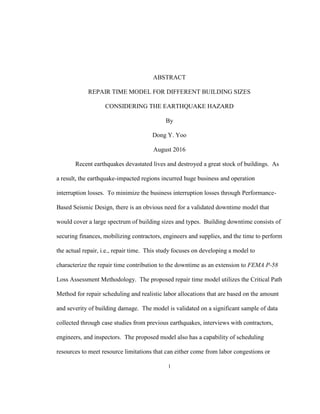
In 2010, Cimellaro, Reinhorn, and Bruneau introduced a quantitative method for
evaluating the resiliency of a building utilizing resiliency index. The resiliency index
represents the capability of a building to sustain a desirable level of functionality over a
period of time decided by owners or society (Cimellaro et al. 2010). It can be calculated
as the normalized area under the functionality curve of a system defined by recovery time
and recovery path (Figure 1). The recovery path is the path that a particular
neighborhood or a community takes to recover from a natural disaster. The recovery
time is defined as the period necessary to restore the functionality of a structure or an
infrastructure system, to a desired level that can operate or function the same, close to, or

3
better than the original one. It is a random variable with high uncertainties that includes
the construction and business recovery and typically depends on the earthquake intensity,
building location and available resources (e.g., capital, materials, and labor), and the
building’s occupancy. The gray shaded area of Figure 1 represents a resilience index for
a structure that is fully operational. After a natural disaster, the functionality diminishes
and is regained to a desired level through a recovery process. To evaluate the resiliency
index of a building, reliable tools for estimating recovery time and recovery path are
needed.
FIGURE 1. Functionality function of a building system after an earthquake.
The recovery time is typically derived from the mobilization time and repair time
(as shown in Figure 1). Mobilization time precedes repair time and includes time required
for building inspection, site preparation, moving of occupants, furnishings and content,

4
engineering services, permitting, financing, contracting construction services, and
acquiring needed material (Comerio 2006). The repair time is the time required to
perform the actual repairs of a structure. Since recovery time is associated with the time
to restore functionality, the actual mobilization and repair times are to be used in
conjunction with the building functionality limit states to map them into their recovery
time contributions (Terzic et al. 2014a; Burton et al. 2015). The functionality limit states
are derived from the damage state of the building to indicate the capacity at which the
intended building function can be maintained in the course of the building repairs.
From the three aforementioned integral parts of the recovery time model, the
focus of this study is on developing a robust and reliable repair time model. The
proposed model is intended to complement FEMA P-58 (FEMA 2000a; FEMA 2000b)
performance assessment methodology and is probabilistic in nature. It is a highly flexible
model with the following capabilities: 1) it is applicable to any building size, 2) it can
accommodate any repair schedule and 3) it optimizes the work-force based on the amount
and severity of damage of building components. The model is validated on a significant
sample of data collected through case studies from previous earthquakes and through
interviews with contractors, engineers, and inspectors specialized in earthquake damage
repair in the Greater Los Angeles area. The final outcome of this study is a realistic
estimation of repair time following an earthquake.
1.1 Organization of Report
This thesis comprises of six chapters. Chapter 2 reviews numerous existing repair
time models (FEMA 2012a; FEMA 2012b; Arup and Arup 2013; Mason et al. 2000;

5
Porter et al. 2001) and explores their strengths and limitations. Chapter 3 provides an
overview of the existing scheduling methodologies and presents a new repair scheduling
methodology developed as a part of this research. Chapter 4 presents the existing
resource scheduling techniques and proposes a new resource scheduling technique that
considers labor congestion during building repairs. Chapter 5 presents the data collected
through the interviews with the contractors, engineers, and inspectors that are used to
calibrate and validate the repair time model. It also presents the work force distribution
that is used for the case studies of 3-story and 12-story office buildings. Chapter 6
presents case studies of 3-story and 12-story office buildings located in the regions of
high seismicity to demonstrate flexibility and robustness of the developed repair time
model. Lastly, the repair times of the proposed model are compared with the repair times
of FEMA P-58 (FEMA, 2012a) repair models to demonstrate the effect of the FEMA P-
58 simplifying assumptions on the results.

6
CHAPTER 2
REVIEW OF EXISTING REPAIR TIME MODELS
The PBEE methodology and its internal modules have been developing over the
last two decades at a high speed to be adopted for general use through FEMA P-58
initiative (FEMA 2012a). With its comprehensive library of peer-reviewed fragility
curves and associated consequence functions for more than 700 structural and
nonstructural building components, FEMA P-58 allows for calculation of numerous
performance metrics including, repair cost, repair time, casualties, and mean annual loss.
From all performance metrics of interest to decision-makers, this study focuses on repair
time and in this chapter discusses four major existing repair time models including
Mason et al. (2000), Porter et al. (2001), FEMA (2012a), and Arup and Arup (2013),
addressing their strengths and limitations.
2.1 Optimal Strategy for Business Recovery after Earthquakes
Mason et al. (2000) proposed a methodology for choosing the best recovery
strategy for a company that owns multiple income-producing properties damaged in an
earthquake. The recovery is optimized by identifying recovery actions that will
maximize the net asset value of the properties owned by the company. The developed
methodology provides a comprehensive framework that can be effectively used in
managing the earthquake recovery. Given the damage states of structural and
nonstructural components of the company-owned units the methodology determines the

7
optimal repair time and optimal expenditure rate assuming the following repair schedule:
all rental units are repaired in parallel and all of the components of a unit are repaired in
series. Although there may be situations that follow the repair sequence assumed in the
study, the repair scheduling following an earthquake is generally more complex.
For example, suppose that company owns 10 units within the building and all
need to be repaired by plumbers and drywall subcontractors. Based on the underlying
assumptions of the methodology, the plumbing and drywall subcontractors will each
assign 10 crews, one for each unit, with drywall crews following the plumber crews. In
case of an earthquake, there is typically a surge in labor demand and there is a greater
chance that each subcontractor will assign only one crew to do the repair of all 10 units
with a drywall crew following the plumbing crew from one unit to another until the repair
of all units is completed. In such situation, the repair sequencing becomes more complex
as there is a great chance that each unit will undergo different amount of plumbing and
drywall damage resulting in wait times of the successor crew.
Since the total repair time is an extremely important variable in strategizing the
business recovery, for the described methodology to provide reliable results, it needs to
be based on realistic repair scheduling that will provide more accurate estimation of the
total repair time. Without the accurate repair time, the optimal asset value will be
inaccurate and may lead to making decisions that will impair the business recovery.
2.2 Assembly-Based Vulnerability (ABV) Methodology
In 2001, Porter, Kiremidjian, and LeGrue introduced assembly-based
vulnerability (ABV) framework for evaluating the seismic vulnerability and performance

8
of buildings on a building-specific basis (Porter et al. 2001). The framework is fully
probabilistic and addresses damage at a highly detailed level utilizing fragility functions
to simulate damage of each structural and nonstructural element in the building, and its
contents. Given the damage state of building components, it uses probabilistic
construction cost estimation and scheduling to estimate repair cost and "loss-of-use
duration" (i.e., a repair time).
ABV framework proposes a repair time model that is based on dividing the
building into individual operational units that independently produce income, such as
rental apartments, office suites, or floors. Each operational unit requires a set of critical
structural, architectural, mechanical, electrical and plumbing features to be functional.
For all critical components of a unit, damage states are combined with repair duration and
probability distributions to estimate the unit repair time using several simplifying
assumptions:
1. Inside an operational unit, crews that are working on the same repair task work
in parallel and crews that are working on different tasks work in series.
2. Repairs are performed in a way that follows Construction Specification
Institute (CSI) MasterFormat standard. For example, structural components must finish
before the start of nonstructural components.
3. Tenants cannot occupy the building until critical repairs are completed and
tenant requirements are neglected while critical components remain unrepaired.
4. In an operational area, only one trade can work at a time. The next trade can
only begin after that trade finishes its work.

9
5. A change-of-trade delay can occur depending on the size and complexity of
the repair and its delay must be considered in the duration.
6. Repairs to different operational units can occur simultaneously if there are
enough resources. The contractor has a choice to work several operational units
simultaneously or sequentially.
The repair time model of ABV framework is novel as it is fully probabilistic and
addresses damage at a highly detailed level. However, the underlying assumptions have
several limitations. The first limitation is in the assumption that repairs are performed in
an order that follows the MasterFormat divisions. This assumption does not consider the
fact that building repairs are different from new constructions and that each building
repair is unique. To accommodate the variability in repair schedules, the user must be
able to estimate the total repair time of a building by using a flexible repair schedule that
allows for an appropriate repair sequencing.
The second limitation is that tenants cannot occupy a building until all critical
repairs are finished. ABV framework does not consider the fact that a building can be
functional when there are critical components with minor damage. In such cases, an
owner may keep the building as functional and avoid a downtime that would result in
economic losses. This limitation can be overcome using functionality limit state ,as
proposed by Terzic et al., 2014a and Burton et al., 2015 that establish if the building is
functional or non-functional during repairs.
The third limitation comes from the assumption that only one trade operates at a
time in an operational area. Although the scenario can certainly occur, it is rare to see

10
only one trade work at a time because it is neither practical nor economical for
subcontractors to operate one at a time. Depending on the size of an operational area,
based on repair schedule and resource availability, different subcontractors should be able
to work together.
In conclusion, ABV framework provides a solid repair time model. However, the
aforementioned assumptions need to be improved to provide more realistic repair time
estimates.
2.3 FEMA P-58: Repair Time Estimation
The PBEE methodology has been recently adopted for general use through FEMA
P-58 initiative (FEMA 2012a) by developing a comprehensive library of peer-reviewed
fragility curves and associated consequence functions considering more than 700
structural and nonstructural building components, using standard methods (Porter et al.
2001) and published data. The motivations behind FEMA P-58 were to improve
accuracy and reliability in performance-based seismic design and to provide metrics for
communicating performances to decision-makers. The methodology is made applicable
to engineers by developing the Performance Assessment Computation Tool (PACT) that
calculates repair cost, repair time, casualties, and probability of unsafe placard (Applied
Technology Council [ATC] 2012).
To perform the loss analysis with PACT, the user first needs to create a
performance model of a building in PACT. The performance model consists of types and
quantities of all structural and nonstructural components, and building contents. In
addition, the user needs to provide basic building information, such as replacement cost,

11
occupancy type, footprint, and story height. The user next provides building structural
responses (maximum story drifts, maximum absolute floor horizontal velocity, maximum
absolute floor horizontal acceleration, and peak residual story drifts) for earthquake
hazard levels or scenarios for which the loss analysis is to be performed.
In PACT, each building component and content is associated with a fragility
curve that correlates structural response to the probability of that item reaching a
particular damage state. The component’s damage is then related to a loss (e.g., repair
cost, repair time) utilizing consequence functions. The total repair loss at a hazard level
or for an earthquake scenario is then estimated by integrating losses over all components
of a system. The estimation of the total repair time at a hazard level is more complex and
will be described in the next paragraph. To account for the many uncertainties affecting
calculation of seismic performance, FEMA P-58 methodology uses the Monte Carlo
procedure to perform loss calculations (FEMA 2012a).
To calculate the total building’s repair time, FEMA P-58 considers two bounding
cases: 1) repair work on all floors begins simultaneously (in parallel) and 2) repair work
of different floors is performed sequentially (in series). In addition, each bounding case
is further simplified with the following two assumptions: 1) repair sequencing at each
floor is assumed to be sequential resulting in a single repair task per floor, and 2) work
force is the same for all repair tasks. In FEMA P-58 it is stated that "Neither strategy is
likely to represent the actual schedule used to repair a particular building, but the two
extremes are expected to represent a reasonable bound to the probable repair time"
(FEMA 2012a). For the simplified and generic scheduling of repairs of FEMA P-58 to

12
provide reasonable bounds, the resources or workers used to estimate the total duration of
work are to be more realistic and several repair trades at a floor should be allowed for the
parallel repair schedule.
FEMA P-58 distributes workers based on worker density, defined in the guideline
as the maximum workers per square foot, recommended to be 0.1% if the building is
occupied during repairs and 0.2% if the building is unoccupied during the repairs. For
example, if a building floor area is 20,000 square feet and worker density is selected to be
0.1%, 20 workers will be assigned to all components that are to be repaired in a building
regardless of the number of damaged units and their damage state. Consider a building
exposed to two ground motion intensities: 1) low intensity of shaking resulting in a
minor damage of one moment connection and moderate damage of partition walls at the
first floor and 2) high intensity of shaking resulting in major damage of 15 moment
connections and severe damage of partition walls at the first floor. Per FEMA P-58 repair
time model, regardless of the intensity of ground shaking and associated damage, 20
workers will be first assigned to repair moment connections and another crew of 20
workers will be next assigned to repair partition walls. Such resource allocation will
result in generous and unrealistic estimates of repair times especially for systems with
minor damage. It is not justifiable to allocate 20 workers to repair only one moment
connection and also to allocate the same crew sizes for repair of moment connections and
partition walls. The same problem will arise by assigning the same crew to all floor
levels as the amount and severity of damage may differ greatly among different floor
levels, especially for taller buildings. In reality, construction practices consider resource

13
constraints that are unique to each repair activity given the amount and severity of
damage in a building as well as the surge in labor demand.
In the probabilistic loss analysis, FEMA P-58 is limited to using constant density
of workers for all realizations of the Monte Carlo simulation process (FEMA 2012a).
The existing repair time model does not allow for different densities of workers for cases
with and without building occupants during the repair. Obviously, for some of the
realizations of the Monte Carlo simulation process, there may be only minor damage that
can be repaired while the building is still occupied. There also may be some realizations
with major damage that will trigger building closure. To distinguish between occupied
and non-occupied cases, functionality limit states could be used (e.g., Terzic et al. 2014a;
Burton et al. 2015).
In FEMA P-58 repair time model, the assumption that only one trade operates at
one floor level, although possible, is rare to see as it is neither practical nor economical
for subcontractors to operate one at a time (e.g., repair of cladding, stairs, and partition
walls can occur simultaneously at one floor level). Depending on the size of the floor
area, type and amount of damage, and resource availability, different subcontractors
should be able to work together.
Finally, assume that the provided bounds of repair time generated by FEMA P-58
were realistic and accurate. The question is would that information be useful in
communication with the decision-makers. Would they be interested to know that the
median repair time for their building is in the range from 9 to 32 days as shown in Figure
2 considering a 12 story steel moment frame building? It is the opinion of the authors

14
that the communication with the decision-makers would be more efficient if a realistic
repair time estimation was possible.
(a)
(b)
FIGURE 2. Median repair time of a 12-story building in (a) parallel schedule and (b)
serial schedule. The median repair time for parallel schedule is about 9 days, while it is
about 32 days for serial schedule.

15
2.4 Arup and Arup's REDi™ Rating System: Repair Time Model
Resilience-based Earthquake Design Initiative (REDi™) Rating System (Arup
and Arup 2103) proposes a framework for owners, architects, and engineers to implement
“resilience-based earthquake design." It describes design and planning criteria to enable
owners to resume business operations and provide livable conditions quickly after an
earthquake, according to their desired resilience objectives. The REDi™ Rating System
utilizes downtime as one of the performance metrics in its “resilience-based earthquake
design." For that purpose they have developed a downtime model that is an extension to
FEMA P-58 methodology. An integral part of their downtime model is a repair time
model that addresses some of the limitations of FEMA P-58 repair time model. However,
REDi™ repair time model still has numerous limitations: fixed repair schedule,
unrealistic labor allocation, and erroneous repair time procedure.
REDi™ adapted a new repair sequence by abandoning the FEMA P-58's parallel
and serial scheduling. In REDi™, components are organized into seven different groups
and the groups are divided into structural, interior repairs, exterior repairs, mechanical
equipment, electrical systems, elevators, and stairs as shown in Table 1. Interior repairs
consist of pipes, HVAC distributions, partitions, and ceiling tiles. Exterior repairs consist
of exterior partitions and cladding or glazing.
The key assumptions in REDi™ methodology are that all structural components
within a building need to be finished repairing before the start of nonstructural repair.
Repair of both structural and nonstructural repair will be scheduled only one floor at the
time starting from the bottom. It is also assumed that temporary elevators are available at

16
the beginning of a project to accommodate materials and equipment during structural
repairs of a building. Repair of components within a group are all sequential and the
relationships between the established groups are fully fixed with no option of regrouping
the repair tasks. Although organizing all components into its groups can be useful, it
inhibits flexibility in scheduling. For example, components inside a structural group can
never work in parallel. In 1994 Northridge earthquake, moment connections and shear-
tab gravity connections of damaged moment frames were typically repaired
simultaneously (Karns 2015). In the same earthquake, the repair of nonstructural damage
would typically start as soon as the structural damage was fixed at the bottom few floors.
It was also very common to start the repair of stairs and elevators simultaneously with
any other structural repair to provide enough routes for transportation of labor and
material. Obviously, every repair work is unique and repair sequencing may vary based
on workers availability, labor congestion, and desired recovery speed specified by the
decision-makers. To accommodate different situations it is important that repair tasks are
considered independently rather than in groups and that flexible relationships exist
between them, both within a floor level and along the building height.
In REDi™, the labor allocation is addressed by introducing labor distributions
that are either based on square footage or number of damaged units (Table 1), capped by
the total number of workers allocated to the project. For repair of structural components,
that start first and are the only trade at the time, they use a metric of 1 worker per 500 sq.
ft. The selected metric aligns with FEMA P-58 recommendation for the workers density
of unoccupied building of 0.2%. Nonstructural components that belong to Sequences A

17
and B are based on 1 worker per 1000 sq. ft because the two sequences can occur
simultaneously, resulting in the total worker density of 0.2%. Repair of sequences C
through F is based on an average number of damaged units.
TABLE 1. Component Subgroups Described in Arup and Arup's REDi™ (2013)
Repair
Sequences
Components
Number of Workers (per sq. ft.
or damaged units)
Structural Structure 1 worker/ 500 sf
Sequence A
Pipes/ Sprinkler
1 worker/ 1000 sf
HVAC distribution
Partitions
Ceilings
Sequence B
Exterior Partitions
1 worker/ 1000 sf
Cladding/Glazing
Sequence C
Mechanical
Equipments
3 workers/damaged unit
Sequence D Electrical Systems 3 workers/damaged unit
Sequence E Elevators 2 workers/damaged unit
Sequence F Stairs 2 workers/damaged unit
In comparison to FEMA P-58 labor allocation, structural components, pipes,
HVAC distribution, partition, ceiling, cladding and glazing are treated the same,
considering the square footage of a floor area. For example, for the floor area of 20,000
sq. ft., regardless of the amount of damage and number of damaged units, 40 workers will
be assigned for the repair of every structural component, and 20 workers will be assigned
for the repair of every aforementioned nonstructural component (Sequences A and B). In
reality, contractors assess the amount of building damage and allocate labor based on a
number of damaged units and their damage states, expected deadline set by the

18
stakeholders, and resource limitations. Therefore, a building with a slight damage will
utilize significantly smaller work force than a building with an extensive amount of
damage.
Per Table 1 of REDi™ document, the repair time calculation is calculated based
on the following procedure:
1. Add direction 1 and 2 repair time values for each drift-sensitive component for
each realization.
2. Obtain median (or desired probability of non-exceedance) loss for each
component at each floor level.
3. At this point, the data has been filtered such that repair times are displayed for
each component at each floor level only.
4. The total repair time estimates are computed by dividing the total number of
‘worker-days’ per floor by the number of workers allocated to each floor and then repairs
across all floors are assumed to occur either simultaneously or only once the repairs on
another floor are completed, starting from the lowest level.
The repair time calculated following the REDi™ procedure is erroneously labeled
as a median repair time and in actuality, the median repair time cannot be interpreted in
statistical terms. The reason is that the median repair times of each component at each
floor level are combined using the repair schedule, generating a result where each
component outcome is associated with a different realization of the Monte Carlo
simulation process as demonstrated in Figure 3. The correct procedure in calculating the
median repair time requires a generation of cumulative distribution functions (CDF) for

19
repair times by utilizing the repair scheduling method for each realization of the Monte
Carlo simulation procedure and the usage of the CDF to calculate the median repair time.
FIGURE 3. Filtering of data in REDi™ procedure. Median values (repair times) of
components A, B, C belong to different realizations of the Monte Carlo simulation
process.
2.5 Conclusion
It is obvious from studies by Mason et al. (2000) and Cimellaro et al. (2010) that
the estimation of the repair time is crucial in measuring the resiliency of a building. In
addition, an accurate estimation can facilitate the stakeholders by providing reliable data
for optimal business decisions.
The repair time models of ABV framework, FEMA P-58, and REDi™ are all
based on sets of simplifying assumptions that are not in agreement with the current
construction practice. There is an obvious need for a robust repair time model applicable
to different building sizes and occupancies that will allow for realistic repair and resource
scheduling.

20
CHAPTER 3
REPAIR SCHEDULING METHODOLOGY
A new repair scheduling method that can accommodate any repair sequencing and
considers realistic labor allocation is presented in this chapter. The repair scheduling
method is developed to work in conjunction with FEMA P-58 methodology and is
applicable to any building size and type, and any intensity of ground shaking. It can be
used in the probabilistic performance-based seismic design of new buildings or for the
evaluation of the existing buildings.
As discussed in Chapter 2, the existing repair time models have several
underlying deficiencies that should be improved upon. The repair time models of ABV
framework, FEMA P-58, and REDi™ are all based on sets of simplifying assumptions
that are not in agreement with the current construction practices. Herein presented repair
time model, applicable to different building sizes and types, is developed in collaboration
with the general contractors to realistically reflect the current construction practices.
To facilitate the development of the new repair time model, different existing
repair scheduling techniques for new construction are investigated and presented in
Section 3.1. Since repair work differs from the new construction, it is essential to
recognize and account for those differences in the new repair time model (Section 3.2).
A new scheduling technique for repair construction is presented in Section 3.3. The
proposed technique is demonstrated on an example that is presented in Section 3.4.

21
3.1 Existing Scheduling Techniques for New Construction
The scheduling techniques that are the most popular in the construction industry
of new buildings are the critical path method (CPM) and the line of balance method
(LOB). To accurately incorporate the repair time model using one of these two
scheduling methods, the advantages and disadvantages of two methods are discussed in
this section.
3.1.1 Critical Path Method
The critical path method is a widely accepted scheduling method in the
construction industry. It provides a way to organize, plan, and identify a number of
activities for the purposes of project management. The CPM is used mainly to identify
the critical activities that make up the shortest duration of the project (Baldwin and
Bordoli 2014). The advantages of the CPM is that it displays all activities, time,
dependencies between activities, and finish dates of all activities. Because of its
simplicity and the ease of use, the CPM was used as a foundation of popular project
management software such as Primavera P6 and Microsoft Project (Christodoulou et al.
2001).
There are two distinct ways of displaying CPM results: using Gantt charts and
network diagrams. Gantt chart is a simple graphical method that shows the progression
of each activity using horizontal bars. In Gantt chart, the duration of each activity is
plotted using a horizontal bar and dependencies between activities are used to plot the
total duration of a construction schedule. The advantages of using a Gantt chart are that
it shows various activities, shows a start and an end date for each activity, shows duration

22
of each activity, shows overlaps between parallel activities, and shows a start and an end
date of an entire project. However, the disadvantages are that it can be difficult to see the
inter-relationships between activities and that it can be convoluted in a project with too
many activities. The second option in displaying the CPM result is using network
diagrams. Network diagrams such as an activity-on-node or a precedence diagram show
the inter-relationship among activities, show detailed information about the sequence,
duration, and free float of each activity, and clearly display the critical path in a project.
However, network diagrams are not an ideal solution for understanding a progression of a
project because the user cannot visualize the project and see the overlaps among
activities. To use the CPM reliably, both Gantt charts and activity-on-node diagrams
should be used to communicate repair schedule in details.
3.1.2 Line of Balance Method
The line of balance (LOB) was first developed to be used in manufacturing
environment for its repetitive nature and was later adapted in repetitive construction
projects (Baldwin and Bordoli 2014). The methodology requires that the production rates
of activities are satisfied by the number of resources assigned to all activities. Each
activity has its own production rate that is determined by the number of resources and the
production rate is graphically shown as a slope of a line in Figure 4. Higher production
rate, defined by a steeper line, generally means that the activity duration is shorter. The
duration of each activity is measured by the difference between the start date at the first
floor and the finish date at the last floor. Because of the linear lines that define the
production rate of each activity, the LOB is perfect for repetitive construction tasks such

23
as a construction of high rise building (Arditi et al. 2002). Because a subcontractor can
progress from the ground level to the top level in a repetitive nature, the LOB is suitable
in showing the production rate and the progression of the subcontractor throughout the
building. For example, the progression and the production rate of a steel fabricator
erecting a high rise building can be plotted as a sloping line in a LOB plot.
FIGURE 4. An example of the line of balance technique. Each line represents an
activity and the slope of a line is defined as the productivity. Flatter lines mean that the
productivity is low and steeper lines mean that the productivity is high.
The advantages of the LOB over the CPM are that the LOB is capable of showing
the production rate and the progression in a single plot. The inability of the CPM to show
the production rate can cause work stoppages, inefficient utilization of resources, and
excessive costs (Arditi et al. 2002). While suitable for a new construction due to its
repetitive nature of tasks, the LOB would be difficult to apply in repair scheduling
because there is a lack of repetitive repair tasks as damage is likely to occur sporadically
1
2
3
1 3 5 7 9 11 13 15 17 19 21 23 25 27
Floors
Days
Line of Balance

24
in different areas and floors of a building. For example, there may be damaged structural
components at first and third floor only, not necessarily across the entire building.
Furthermore, with the LOB graphs it is difficult to understand the inter-relationships
between activities and to read when there are overlapping activities with the same
production rates.
From the two presented scheduling techniques, the CPM is a preferred method as
it has capability to convey repair scheduling information clearly. Therefore, the CPM
with the Gantt chart and an activity-on-node diagram is selected to be used in the repair
time model. The Gantt chart will be used to show the progression of the repair and the
critical activities. The network diagrams will be used to highlight the inter-relationships
between activities in each floor.
3.2 Differences Between New Construction and Repair Work
The repair of a building with an earthquake-induced damage differs greatly from
the new construction. The damage is likely to occur sporadically in different areas and
floors of a building. This results in a repair schedule that is not repetitive in nature.
While the number of repair tasks and the number of resources assigned to each activity
may be different at different floors of the damaged building, the number of activities and
the number of resources in new constructions of a high-rise building are likely to remain
constant throughout all floors.
For the earthquake-induced damage with limited space availability inside a
building, the repair construction is typically slower than the new construction. Limited
space poses difficulties in setting up equipment, it slows down contractors, and reduces

25
their productivity. For example, a building that has a significant damage to pre-cast
concrete stairs can pose a challenge to a contractor. First, they may need to remove stairs
out of a building by disassembling the stairs. Removing the stairs in a confined space
may require additional work done by the contractor such as disassembling the stairs into
smaller pieces to fit the openings and entrances of the building. Finally, the new stairs
are to be installed.
In the case of an earthquake that impacts large urban regions, the number of
available workers may be reduced due to a surge in construction demand after a disaster.
The surge in construction demand will pose difficulties to building owners in securing
contractors. Furthermore, due to a high demand, contractors may be tempted to secure
more jobs by reducing number of workers allocated at each project.
3.3 Repair Scheduling Method
Although there is a significant body of research work that relates to the new
construction, the research work on repair scheduling is quite scarce (see Chapter 2). The
new repair scheduling method for buildings with earthquake-induced damage is presented
in this section. The method uses CPM with Gantt chart and activity-on-node diagram and
is created and validated with a help from general contractors, inspectors, and structural
engineers around the Greater Los Angeles area with significant experience in earthquake
repair of buildings. The method is developed to work in conjunction with seismic
performance assessment methodology of FEMA P-58. Terms and definitions that are
widely used in the construction industry are defined in Section 3.3.1. Initial parameters
associated with the developed repair scheduling method are stated in Section 3.3.2. The
repair scheduling method is presented in Section 3.3.3.

26
3.3.1 Terms and Definitions
Prior to the introduction of the new repair scheduling method it is necessary to
define terms that will be used throughout this document. The presented terms are widely
used in the construction industry (Caltrans 2003; Baldwin and Bordoli 2014) and are
common language for contractors. However, the method is developed to be used by
structural engineers in the performance-based seismic design of new buildings or for the
evaluation of the existing buildings, and therefore necessitates terms definitions.
Activity: A task or event that contributes to a completion of a project. Each
activity should have its unique activity number.
Predecessor activity (Predecessor): An activity which controls the start date of
the following activity. Only the first activity does not have a predecessor.
Successor activity (Successor): An activity that cannot start until the completion
of the activity before it. Only the last activity does not have a successor.
Finish-to-start (FS) relationship: The successor activity cannot start until the
predecessor finishes.
Start-to-start (SS) relationship: The successor activity cannot start until the
predecessor starts.
Finish-to-finish (FF) relationship: The successor activity finishes at the same
time as the predecessor.
Start-to-finish (SF) relationship: The successor activity finishes after the start of
the predecessors.

27
Early Dates: Within constraints, resources and logic of a network, these dates
represent the earliest start and finish dates for activities or sequences of activities
(Baldwin and Bordoli, 2014).
Late Dates: Within constraints, resources and logic of a network, these dates
represent the latest start and latest dates for activities or sequences of activities.
Forward Pass: The forward pass is used to calculate early dates of each activity in
a schedule.
Backward Pass: The backward pass is used to calculate late dates of each activity
in a schedule.
Total Float: Total float is the measure of time (work days) a project can be
delayed without delaying the project completion date.
Free Float: Free float (FF) is the measure of time (work days) a predecessor
activity can be delayed without delaying its successor activity. Free float is calculated
using only early dates in the forward pass.
Logic Network: Logic network is a dependency diagram that shows
dependencies among linking activities in a construction schedule. The logic network
must be robust to avoid any out-of-sequence progress and illogical construction schedule.
3.3.2 Initial Parameters
In order to effectively implement the repair scheduling method that is realistic and
flexible, several initial parameters that define the logic networks must be defined.
All predecessor activities must be defined first. A predecessor activity is any
activity that controls the start of the following activity. The start of an activity can be

28
controlled in two ways. First scenario is when a predecessor activity must finish before
the start of an activity. For example, if in the logic network it is determined that Activity
A must finish before the start of Activity B, Activity A is the predecessor of Activity B.
This situation is typical for repair activities within the same floor of a building. The
second scenario is when an activity must finish before it can start at the next floor level.
For example, consider a situation where Activity A must finish before the start of
Activity B at each floor and a building has three floors. According to this scenario,
Activity A at the first floor must finish before the same activity can start at the second
floor and this relationship would continue until the last floor level. Similarly, Activity B
at the first floor cannot start until Activity A at the first floor finishes and this follows the
typical relationship that defines the predecessor activity. However, Activity B at the
second floor cannot continue unless Activity A at the second floor is finished and
Activity B at the first floor is finished. Therefore, the start of Activity B at the second is
governed by finish date of Activity A at the first floor and the finish date of Activity B at
the second floor. This is the second type of predecessor relationships that must continue
until the last floor level. .
All successor activities must be defined next. A successor activity is an activity
that cannot start until the completion of the activity before it. Successor activities are
essential in calculation of free floats which are the measure of time a predecessor
activities can be delayed without delaying its successor activities. Free floats are
important during the resource scheduling method that is presented in Chapter 4.
While the new construction typically progresses one floor at a time, the repair

29
construction often progresses across several floors simultaneously. To assure flexibility
in repair scheduling, the developed model allows specification of the number of floors
that are simultaneously repaired for each repair activity.
3.3.3 Repair Scheduling Method
The new repair scheduling method for buildings with earthquake-induced damage
is presented in this section. The method uses CPM and is based on several assumptions
common for construction scheduling:
1. The activities are time-continuous and thus once started they cannot be
interrupted.
2. The resource assignments for each activity are assumed constant throughout
the duration of the activity.
3. The project’s logic network is constant throughout all floors.
4. All activities are based on Finish to Start (FS) relationship.
The method is developed to work in conjunction with probabilistic seismic
performance assessment methodology of FEMA P-58 (see Section 2.3). Therefore, for
the repair scheduling method to be utilized it is necessary to: 1) create a performance
model of a building in PACT including specification of types and quantities of all
structural and non-structural components, and building contents; 2) provide building
structural responses (maximum story drifts, maximum absolute floor horizontal velocity,
maximum absolute floor horizontal acceleration, and peak residual story drifts) for
earthquake hazard levels or scenarios for which the loss analysis is to be performed, and
3) execute the analysis with PACT to generate the input data necessary for the repair time

30
estimation including: repair time durations, number of damage units, and damage states
of all building components. Repair time durations in PACT are based on the metric of 1
day per 1 worker. Depending on the severity and amount of damage, the repair time
durations generated by PACT are to be modified using realistic labor allocations. For
each building component, the labor allocation will be determined based on the severity of
damage utilizing the average damage state of a component and amount of damage
utilizing the number of damaged units.
The repair scheduling method that is to be used for calculation of the repair time
of an earthquake damaged building is presented next (see Figure 5 for the flow chart):
Step 1. Set the logic network for repair by defining predecessor and successor
relationships for all repair activities and defining the number of floors repaired
simultaneously for each repair activities. The methodology allows a scheduling repairs
of several floors simultaneously.
Step 2. Import the following information from PACT: repair time durations,
number of damaged units (NDU) and corresponding damage states (DM) for all
components at every floor of a building for all realizations of the Monte Carlo simulation
process.
Step 3. Calculate the average damage states (ADS) of all repair activities at each
floor for all realizations. An average damage state of a building component is calculated
as follows:
𝑨𝑫𝑺 =
∑ 𝒏 𝒊 𝑫𝑴 𝒊
𝒌
𝟏
𝒏
( 3.1 )

31
where n is a total number of units associated with a component of one floor level, k is the
total number of damages states of that component, and ni is the number of units in
damage state i.
Step 4. For all components at each floor level and all realizations, assign the
number of workers to repair of a component based on its average damage state (ADS)
and a number of damaged units (NDU). The total number of workers is calculated as a
multiple of the number of crews and number of workers within a crew. The number of
workers within a crew is defined based on the average damage state and the number of
crews is defined based on the number of damaged units. Table 2 shows an example of
possible work allocation for a building component A. In this example, if ADS is less
than 1, two workers are assigned and if ADS is greater than 1, three workers are assigned
for each crew. Then, the number of crews is assigned based on NDU. Consider the
following scenarios: 1) if there are 20 damaged units with ADS < 1, two crews of two
workers resulting in total of 4 workers, are used, and 2) if there are 21 or more damaged
units with ADS > 1, three crews of three workers resulting in total of 9 workers, are used.
For a realistic labor allocation it is recommended that the user populates the data of Table
2 in consultation with a general contractor.
TABLE 2. Sample Worker Allocation
Component Names
Workers per Crew (Based on
ADS)
Total workers based on NDU and ADS
ADS < 1
1 < ADS
< 2
2 < ADS <
3
# of damaged units in a floor
1 - 10 11 - 20 21 - 30
Component A 2 3 3 1 Crew 2 Crews 3 Crews

32
Step 5. Calculate final repair durations of all activities by dividing total repair
durations (hours / 1 worker) by the number of workers that is assigned in Step 4.
Step 6. For each realization of the Monte Carlo simulation loss assessment
procedure use the repair logic network along with the final repair times off all activities
to calculate the duration of building repairs based on the following procedure:
Firstly, use the predecessor relationships and the repair time durations to calculate
the starting and finish dates of all activities. When there are multiple predecessors, a
predecessor with a bigger finish date is set as the start date of an activity. Start dates and
finish dates are calculated as follows:
𝑆𝑡𝑎𝑟𝑡 𝐷𝑎𝑡𝑒 𝐴,𝑓𝑙𝑜𝑜𝑟 # = max(𝐹𝑖𝑛𝑖𝑠ℎ 𝐷𝑎𝑡𝑒 𝑃𝑟𝑒𝑑𝑒𝑐𝑒𝑠𝑠𝑜𝑟) ( 3.2 )
𝐹𝑖𝑛𝑖𝑠ℎ 𝐷𝑎𝑡𝑒 𝐴,𝑓𝑙𝑜𝑜𝑟 # = 𝑆𝑡𝑎𝑟𝑡 𝐷𝑎𝑡𝑒 𝐴,𝑓𝑙𝑜𝑜𝑟 # + 𝐷𝑢𝑟𝑎𝑡𝑖𝑜𝑛 𝐴,𝑓𝑙𝑜𝑜𝑟 # ( 3.3 )
Secondly, calculate Free Float of each activity using successor relationships and a
forward pass. Free float of a component is calculated as
𝐹𝐹𝐴,1𝑠𝑡 𝑓𝑙𝑟. = 𝑆𝑡𝑎𝑟𝑡 𝑇𝑖𝑚𝑒 𝐸𝑎𝑟𝑙𝑖𝑒𝑠𝑡 𝑆𝑢𝑐𝑐𝑒𝑠𝑠𝑜𝑟 − 𝐹𝑖𝑛𝑖𝑠ℎ 𝑇𝑖𝑚𝑒 𝐴,𝑓𝑙𝑜𝑜𝑟 ( 3.4 )
Thirdly, begin resource scheduling. Refer to Chapter 4 for methodology.
Lastly, determine the critical path and the total duration of the repair project.
Step 7. Generate cumulative distribution functions (CDF) associated with the
duration of the repair project, i.e., repair time.
Step 8. Plot the start dates and finish dates for all activities at all floors including
a roof level.

33
FIGURE 5. Flowchart of the proposed repair scheduling methodology. The flowchart
applies to one realization of the Monte Carlo simulation process within FEMA P-58 loss
assessment methodology.

34
3.4 Example of Repair Scheduling
To demonstrate the flexibility of the proposed repair scheduling method a
simplified and generic example is created. A 3-story building with 3 structural and 7
nonstructural components is used in this example. This example was simplified by using
arbitrary repair durations and resources. Although the resource distribution method that
is introduced in the proposed methodology is one of the key improvements from the
existing repair models mentioned in Chapter 2, the resources were arbitrarily assigned to
avoid a building-specific discussion that is made in the case studies. The case studies of
3-story and 12-story buildings are presented in Chapter 5.
For this generic example it is assumed that activities A, B, and C are structural
components and that activities D through J are nonstructural components (Figure 6). It is
also assumed that activity J is the only nonstructural component that is located at the roof
level. In addition, it is assumed that the structural components are repaired
simultaneously at all three floors and nonstructural components are repaired sequentially
at each floor. The dependencies and inter-relationships among all activities are shown in
Figure 7 in a form of an activity-on-node diagram.
3.4.1 Initial Parameters
The initial parameters of a repair scheduling, including the predecessors,
successors, and a number of floors being repaired simultaneously for each activity are
presented in Table 3 and are based on the repair scheduling example presented in Figures
6 and 7.

35
FIGURE 6. Repair Schedule of a generic example.

36
FIGURE 7. Activity-on-node diagram of a generic example.
TABLE 3. Initial Parameters of All Activities Listed in the Example.
Activity ID Activity Name Predecessors Successors
Floors Repaired
Simultaneously
1 A - 4, 7, 9, 10 3
2 B - 4, 7, 9, 10 3
3 C - 4, 7, 9, 10 3
4 D 1, 2, 3 5 1
5 E 4 6 1
6 F 5 - 1
7 G 1, 2, 3 8 1
8 H 7 - 1
9 I 1, 2, 3 - 1
10 J 1, 2, 3 - 1

37
3.4.2 Repair Time Durations and Resources
To use the repair scheduling method in conjunction with FEMA P-58, repair
durations (𝑤𝑜𝑟𝑘 𝑑𝑎𝑦/(1 𝑤𝑜𝑟𝑘𝑒𝑟)), damage states (DM) and a number of damaged unit
(NDU) need to be imported from PACT. Then, average damage states (ADS) are to be
calculated for each activity at each floor and a number of workers for all activities are to
be assigned based on ADS and NDU. In this generic example, NDU and DM are not
available and therefore, a number of workers cannot be assigned based on ADS and
NDU. However, to demonstrate the flexibility of the repair scheduling method, the repair
durations and resources are assigned arbitrarily for all activities as shown in Table 4. For
structural activities A, B, and C, four workers are required to form a crew and all three
floors are repaired simultaneously. For the rest of nonstructural activities, only one crew
is assigned to repair each floor sequentially. The repair durations and resources are
selected to highlight interesting inter-relationships in a schedule.
TABLE 4. Arbitrary Repair Durations and Resources (Number of Workers) of Each
Activity
Activity
ID
Activity
Name
Repair Duration
(work days / 1 worker)
Resources (workers)
(Based on ADS and NDU)
Floor
1
Floor
2
Floor
3
Floor
1
Floor
2
Floor
3
1 A 160 92 120 4 (1 crew) 4 (1 crew) 4 (1 crew)
2 B 150 100 136 4 (1 crew) 4 (1 crew) 4 (1 crew)
3 C 200 112 140 8 (2 crew) 4 (1 crew) 4 (1 crew)
4 D 18 20 10 1 (1 crew) 1 (1 crew) 1 (1 crew)
5 E 40 10 20 2 (1 crew) 2 (1 crew) 2 (1 crew)
6 F 90 20 57 3 (1 crew) 3 (1 crew) 3 (1 crew)
7 G 40 80 68 7 (1 crew) 7 (1 crew) 7 (1 crew)
8 H 60 16 20 3 (1 crew) 3 (1 crew) 3 (1 crew)
9 I 38 18 20 2 (1 crew) 2 (1 crew) 2 (1 crew)
10 J 0 0 26 2 (1 crew) 2 (1 crew) 2 (1 crew)

38
3.4.3 Repair Time Calculations Based on CPM
Using the initial parameters listed in Table 3 and the repair duration and resources
of Table 4, the start dates, finish dates, and floats are established for each activity based
on CPM. Final durations of all activities are shown in Table 5 and the start dates, finish
dates, and floats are shown in Table 6. In this example, only several activities are
calculated to demonstrate the computations.
Calculations of activity A at 1st floor are shown below. The start date of activity
A at 1st floor is at 0 days.
𝑆𝑡𝑎𝑟𝑡 𝐷𝑎𝑡𝑒 𝐴,𝑓𝑙𝑜𝑜𝑟 1 = 0 ( 3.5 )
𝐷𝑢𝑟𝑎𝑡𝑖𝑜𝑛 𝐴,𝑓𝑙𝑜𝑜𝑟 1 =
𝑂𝑟𝑖𝑔𝑖𝑛𝑎𝑙 𝐷𝑢𝑟𝑎𝑡𝑖𝑜𝑛 𝐴,𝑓𝑙𝑜𝑜𝑟 1
𝑅𝑒𝑠𝑜𝑢𝑟𝑐𝑒 𝐴,𝑓𝑙𝑜𝑜𝑟 1
=
160 𝑑𝑎𝑦𝑠
4 𝑤𝑜𝑟𝑘𝑒𝑟𝑠
= 40 𝑑𝑎𝑦𝑠 ( 3.6 )
𝐹𝑖𝑛𝑖𝑠ℎ 𝐷𝑎𝑡𝑒 𝐴,𝑓𝑙𝑜𝑜𝑟 1 = 𝑆𝑡𝑎𝑟𝑡 𝐷𝑎𝑡𝑒 𝐴,𝑓𝑙𝑜𝑜𝑟 1 + 𝐷𝑢𝑟𝑎𝑡𝑖𝑜𝑛 𝐴,𝑓𝑙𝑜𝑜𝑟 1
= 0 + 40 = 40 𝑑𝑎𝑦𝑠 ( 3.7 )
Because activities A, B, and C are repaired simultaneously at all three floors, the start
date of all three activities at all three floors is 0 day. Similar calculations are performed
with different durations for activities B and C.
Calculations of activity D are shown below. Because activity D is the first
nonstructural component that follows the repair of structural components, the start date of
activity D at first floor is governed by the latest date of structural repairs at the first floor.
The start date of activity D at 1st floor is governed by activity A at 40 days.
𝑆𝑡𝑎𝑟𝑡 𝐷𝑎𝑡𝑒 𝐷,𝑓𝑙𝑜𝑜𝑟 1 = 40 days ( 3.8 )
𝐷𝑢𝑟𝑎𝑡𝑖𝑜𝑛 𝐷,𝑓𝑙𝑜𝑜𝑟 1 =
𝑂𝑟𝑖𝑔𝑖𝑛𝑎𝑙 𝐷𝑢𝑟𝑎𝑡𝑖𝑜𝑛 𝐷,𝑓𝑙𝑜𝑜𝑟 1
𝑅𝑒𝑠𝑜𝑢𝑟𝑐𝑒 𝐷,𝑓𝑙𝑜𝑜𝑟 1
=
18 𝑑𝑎𝑦𝑠
= 18 𝑑𝑎𝑦𝑠 ( 3.9 )

39
𝐹𝑖𝑛𝑖𝑠ℎ 𝐷𝑎𝑡𝑒 𝐷,𝑓𝑙𝑜𝑜𝑟 1 = 𝑆𝑡𝑎𝑟𝑡 𝐷𝑎𝑡𝑒 𝐷,𝑓𝑙𝑜𝑜𝑟 1 + 𝐷𝑢𝑟𝑎𝑡𝑖𝑜𝑛 𝐷,𝑓𝑙𝑜𝑜𝑟 1
= 40 + 18 = 58 𝑑𝑎𝑦𝑠 ( 3.10 )
As shown in Figure 7, the start of activity D is determined by either the finish of
structural components at the second floor or the finish of activity D at the first floor. In
this case, the start date of activity D at 2nd floor is governed by the finish of activity D at
the first floor, which is at 58 days.
=
20 𝑑𝑎𝑦𝑠
= 20 𝑑𝑎𝑦𝑠 ( 3.12 )
= 58 + 20 = 78 𝑑𝑎𝑦𝑠 ( 3.13 )
Again, the start date of Activity D at third floor is governed by the finish of activity D at
the second floor, which is at 78 days.
=
10 𝑑𝑎𝑦𝑠
= 10 𝑑𝑎𝑦𝑠 ( 3.15 )
= 78 + 10 = 88 𝑑𝑎𝑦𝑠 ( 3.16 )
Based on this calculation, the workers that are repairing activity D are finished in 88 days.
Calculations of Activity E are shown below. At the first floor, the start date of
activity E is governed by the finish date of activity D at 58 days.
𝑆𝑡𝑎𝑟𝑡 𝐷𝑎𝑡𝑒 𝐸,𝑓𝑙𝑜𝑜𝑟 1 = 58 days ( 3.17 )
𝐷𝑢𝑟𝑎𝑡𝑖𝑜𝑛 𝐸,𝑓𝑙𝑜𝑜𝑟 1 =
𝑂𝑟𝑖𝑔𝑖𝑛𝑎𝑙 𝐷𝑢𝑟𝑎𝑡𝑖𝑜𝑛 𝐸,𝑓𝑙𝑜𝑜𝑟 1
𝑅𝑒𝑠𝑜𝑢𝑟𝑐𝑒 𝐸,𝑓𝑙𝑜𝑜𝑟 1
=
40 𝑑𝑎𝑦𝑠
= 20 𝑑𝑎𝑦𝑠 ( 3.18 )

40
𝐹𝑖𝑛𝑖𝑠ℎ 𝐷𝑎𝑡𝑒 𝐸,𝑓𝑙𝑜𝑜𝑟 1 = 𝑆𝑡𝑎𝑟𝑡 𝐷𝑎𝑡𝑒 𝐸,𝑓𝑙𝑜𝑜𝑟 1 + 𝐷𝑢𝑟𝑎𝑡𝑖𝑜𝑛 𝐸,𝑓𝑙𝑜𝑜𝑟 1
= 58 + 20 = 78 𝑑𝑎𝑦𝑠 ( 3.19 )
The start date of activity E at second floor is governed by the finish date of activity E at
the first floor or the finish date of activity D at the second floor. In this particular
example, the finish dates of two activities are same. Therefore, the start date of Activity
E at 2nd floor is at 78 days.
=
10 𝑑𝑎𝑦𝑠
= 5 𝑑𝑎𝑦𝑠
= 78 + 5 = 83 𝑑𝑎𝑦𝑠 ( 3.21 )
At third floor, the start date of activity E is governed by the finish date of activity E at the
second floor or the finish of activity D at the third floor. Comparing the finish date of 88
days by activity D and 83 days by activity E, the start date of activity E at 3rd floor is
governed by activity D at 88 days.
=
20 𝑑𝑎𝑦𝑠
= 10 𝑑𝑎𝑦𝑠 ( 3.23 )
= 88 + 10 = 98 𝑑𝑎𝑦𝑠 ( 3.24 )
Using the CPM, the user can quickly calculate the start and finish dates of all activities.
Tables 5 and 6 show the final results.

41
TABLE 5. Repair Durations, Resources (Number of Workers) and Final Durations
Activity
ID
Activity
Name
Repair Durations
(Days / 1 worker)
Resources
Final Repair Duration
Floor
1
Floor
2
Floor
3
Floor
1
Floor
2
Floor
3
Floor
1
Floor
2
Floor
3
1 A 160 92 120 4 4 4 40 23 30
2 B 150 100 136 4 4 4 38 25 34
3 C 200 112 140 8 4 4 25 28 35
4 D 18 20 10 1 1 1 18 20 10
5 E 40 10 20 2 2 2 20 5 10
6 F 90 20 57 3 3 3 30 7 19
7 G 40 80 68 7 7 7 6 12 10
8 H 60 16 20 3 3 3 20 6 7
9 I 38 18 20 2 2 2 19 9 10
10 J 0 0 26 2 2 2 0 0 13
TABLE 6. Start Date, Finish Date, and Free Float of All Activities
Activity
ID
Activity
Name
Start Date Finish Date Free Float
Floor
1
Floor
2
Floor
3
Floor
1
Floor
2
Floor
3
Floor
1
Floor
2
Floor
3
1 A 0 0 0 40 23 30 0 17 10
2 B 0 0 0 38 25 34 2 15 6
3 C 0 0 0 25 28 35 15 12 5
4 D 40 58 78 58 78 88 0 0 0
5 E 58 78 88 78 83 98 0 5 17
6 F 78 108 115 108 115 134 0 0 0
7 G 40 46 58 46 58 68 0 0 4
8 H 46 66 72 66 72 79 0 0 55
9 I 40 59 68 59 68 78 0 0 56
10 J NA NA 40 NA NA 53 0 0 81

42
3.4.4 Results
The repair schedule of a generic 3-story building are displayed using Gantt chart
(Figure 8). The chart shows that the structural components A, B, and C are repaired
simultaneously at the beginning of the project for all floors. As soon as the repair of the
governing structural component (activity A) is finished at the first floor, the repair of
nonstructural components D, G, and I begins simultaneously at the first floor. Repair
activity J that is located at the roof starts following the completion of all structural repairs
within the building.
FIGURE 8. Repair schedule displayed using Gantt chart of a generic 3-story building.
The start date of each activity is governed by the maximum of either the finish
date of the same activity in the floor below or the finish date of the predecessor activity in
the same floor. For example, the repair of component F in second floor does not start
until the crew finishes repairing at the first floor.
In this generic example, the critical path of this repair is associated with the repair

43
activities A, D, E, and F. Components such as B, C, and H have free floats (FF) available
to extend or stretch if the labor congestion requires the use of the resource scheduling
method. Stretching of these activities with FF may not affect the finish time of a project
and stretching can be used to reduce the congestion.
3.5 Conclusion
The proposed scheduling method is flexible, simple, and robust. The flexibility is
provided by allowing the user to set any schedule and any number of workers for any
activity based on the unique repair situation. Therefore, this proposed method can be
used for a building of any type and size. The simplicity of the procedure allows for a
visual presentation utilizing the Gantt chart, an identification of the critical path during
the repair, and an identification of the major contributors to the repair time. The
robustness of the repair scheduling algorithm allows for a simultaneous calculation of
repair times for thousands of realizations of the Monte Carlo simulation process utilized
within FEMA P-58 loss assessment methodology.
The proposed repair scheduling method encourages more collaboration between
engineers, general contractors, and building owners during the design process. By
allowing the identification of the major contributors to the repair time, it facilitates the
design process in meeting unique performance objectives set by the building owner. It is
also greatly beneficial to stakeholders when making cost-benefit analysis of different
structural systems as it allows for estimation of indirect losses.

44
CHAPTER 4
RESOURCE SCHEDULING METHOD
The resource scheduling is crucial in construction industry because using an
optimum number of resources is the key to a successful project that is efficient and cost-
effective. Using the optimum resources can increase the productivity, avoid project
delays, and maximize the profit by avoiding excessive costs of a project. A new resource
scheduling method that addresses labor congestions during the repairs is presented in this
chapter.
The existing repair time models introduced in Chapter 2 use several underlying
assumptions that should be improved. In FEMA P-58, regardless of the severity of
ground shaking and associated damage, assigned resources for each activity are always
assumed to utilize the maximum capacity of the workers that can simultaneously operate
without causing the labor congestion. For example, if a building floor area is 20,000
square feet and worker density is selected to be 0.1%, 20 workers will be assigned to each
components that is to be repaired in a building regardless of the number of damaged units
and their damage state. Such assumption guarantees that the repair is performed with the
maximum labor capacity and that the labor congestion never occurs. In reality,
construction practices consider resource constraints that are unique to each repair activity
given the amount and severity of damage in a building as well as the surge in labor
demand. In REDi™ by Arup, worker distributions are based on either the square footage

45
or the number of damaged units. Though having two ways of distributing labor is an
improvement from FEMA P-58 methodology, REDi™ repair time model is also based on
the assumption that the total number of workers allocated to the project is capped off by
the maximum feasible worker density. Consequently, neither FEMA P-58 nor REDi™
will experience labor congestion as both methods use a predefined capacity that
guarantees perfect labor distributions regardless of the severity of the damage and the
number of damaged components. This is neither realistic nor practical in construction
practices.
Given that the proposed repair time model (presented in Chapter 3) uses flexible
repair scheduling and allocates workers to a damaged component based on the number of
damaged units (NDU) and the average damage state (ADS), labor congestion may occur
in a heavily damaged building. To address the labor congestion, a new, relatively simple,
and computationally efficient resource scheduling method is develop to work with the
probabilistic Monte Carlo simulation process of FEMA P-58. The method can also work
in conjunction with the building functionality limit state (e.g., Terzic et al. (2015); Burton
et al. (2015)) that distinguishes between an occupied and unoccupied building during the
repairs which in turn can be used to set a daily resource limit.
To facilitate the development of the new resource scheduling methods, different
existing resource scheduling methods for the new construction are investigated and
presented in Section 4.1. The new resource scheduling method is presented in Section
4.2. The proposed technique is demonstrated on the example that is a continuation of the
generic example from Section 3.4 and is presented in Section 4.3.

46
4.1 Existing Resource Scheduling Methodologies
Different resource scheduling methodologies are discussed in this section. Firstly,
several different resource graphing techniques (Gordon and Tulip, 1997) are discussed to
guide readers through the basics of resource scheduling (Section 4.1.1). Then, more
complex Packing method by Harris (1994) and Modified Minimum Moment method by
Hiyassat (2000) are presented in Sections 4.1.2. and 4.1.3., respectively. Different
variations of the resource scheduling methodologies are explored to find the most suitable
method for the proposed repair scheduling method.
4.1.1. Overview of Different Resource Modeling and Graphing Techniques
To understand the complex resource scheduling methodologies, the resource
modeling or graphing techniques need to be explained first. In this section, five different
resource modeling techniques are discussed based on the paper published by Gordon and
Tulip (1997).
The first resource method utilizes an aggregation approach to determine how
many resources are used on a daily basis by aggregating the resources used in all
activities. For example, Figure 9 shows that there are a total of 4 resources used in day 1,
3 resources in day 2, 2 resources in day 3 and so forth. The resources are typically
presented in a histogram to highlight the peaks and valleys of the resources during the
project duration. The aggregation method is useful in showing the total number of
workers throughout a project and can be effectively used in conjunction with a Gantt
chart. The method is very helpful in identifying the activities that are exceeding the
resource limitation.

47
FIGURE 9. Example of a histogram in an aggregation method. Number of workers for
each activity is aggregated.
The second method is an accumulation method. Its objective is to provide a
running accumulation of the resources during the life of the project. The method of
calculating the total resources required for each day is the same as that of aggregation
method. The only significant difference is in the graphical representation, as the
resources for any day of the project show cumulative resources from the beginning of the
project until the considered day of the project (Figure 10). For example, the number of
accumulated resources on Day 1 is 4 workers and on Day 2 is 7 workers (the sum of the
resources from Days 1 and 2 in Figure 9). Although this method can be used to show the
cumulative distribution of resources, it does not have a capability of identifying the
components that exceed the daily resource limit and is not suitable for the use within the
proposed repair scheduling method.

48
FIGURE 10. Example of a histogram in an accumulation method.
The third method is an allocation method. Its objective is to provide a feasible
schedule for the completion of the project within the management constraints.
Management constraints are instigated by either the time-limited schedule or the
resource-limited schedule. The time-limited schedule is present when the project
duration must not extend beyond its limits and unlimited resources are allocated to meet a
demand of an end date. The resource-limited schedules is present when a limited amount
of resources is available and the project duration is allowed to extend beyond the end
project date based on the limited resources. For example, when a project is time-limited,
each activity with an unlimited number of resources is allocated to meet the project’s
network logic and the final project deadline that is predefined. On the other hand, when a
project is resource-limited, each activity with a limited number of resources is allocated
to satisfy the network logic and the project can be extended. In the proposed repair
scheduling method, the resource-limited allocation method can be used appropriately to

49
address the surge in labor demand after a disaster and to support realistic and reliable
repair time model. However, the time-limited allocation method is not appropriate
because of the unrealistic assumption of unlimited resources.
The fourth method is a smoothing method. Its objective is to produce a schedule
with a uniform level of resources. It is an iterative process that repeats until all activities
are scheduled based on the following steps. First, only critical activities are scheduled
and allocated in a resource histogram. Then, each noncritical activity is scheduled based
on the availability of free floats between activities and the uniformity in the resource
histogram. Lastly, start dates, finish dates, and free floats of all activities are adjusted for
the noncritical activities that have not been scheduled until all of the noncritical activities
are finished scheduling. The smoothing method is used to form a uniform level of
resources and is inappropriate for the repair scheduling method given that the earthquake
damage likely occurs sporadically at different floor levels, creating non-uniform
distribution of workers at each floor. Therefore, this iterative and computationally heavy
method may never reach uniform distribution in case of an earthquake repair.
The fifth method is called leveling. Its objective is to remove the peaks and
valleys of a resource schedule commonly present in many resource scheduling methods.
This method is an iterative method that checks the resource profile in a resource
histogram, finds the highest point on the profile, identifies the activities at the highest
point on the profile, and moves each contributing activity around to reduce peaks until all
of the peaks and valleys are eliminated in a resource histogram. Although this method
has features that could be adopted within the repair scheduling method, the iterative

50
nature of this approach may require heavy computations for the cases of heavy damage.
4.1.2 Packing Method for Resource Leveling (PACK)
This section presents Packing Method for Resource Leveling (PACK) developed
by Harris (1994). PACT is a heuristic method that is simple and easy to use by the
construction managers. The main objectives of his method are to schedule project
activities to accommodate the fixed project terminal date and to keep the variation in the
daily resources to its minimum. PACK method assigns resources to specific days so that
the peaks and valleys of the resource histogram are reduced.
The assumptions made in PACK method are listed below:
1. Activities are assumed to be time continuous. Once an activity is started, it is
expected that it will continue to completion without interruption.
2. Resources applied to each activity are assumed to remain constant throughout
the duration of the activity. Thus, an activity will have a constant rate of utilization of the
resource.
3. The duration of each activity is assumed to remain constant. Once the duration
is established, no reduction or extension of the duration is permitted by a change in the
activity's resource rate.
4. The logic network is assumed fixed. The network may be cast in either arrow
or precedence form, although the heuristic is presented using the precedence network.
Any logical relationship may exist between any two activities and multiple relationships
are acceptable.

51
5. The project's terminal date is assumed fixed. The heuristic does not extend or
shorten the project duration.
The assumptions 1 through 4 are present in the repair construction and are
therefore adopted within the proposed repair scheduling method (presented in Chapter 3).
However, the final assumption that the finish date is assumed fixed is not common for the
repair construction and is therefore removed to allow for a stretching of the project
duration based on labor congestions. Although PACK is a great method for a new
construction that is typically time-limited, it has limited application in the repair
construction that are typically resource-limited. PACK only levels resources by removing
peaks and valleys of daily resources and moving the activities within their free floats to
keep the variation of daily resources to its minimum while keeping the project’s terminal
date fixed. It does not have a capability of scheduling the construction where resource
limits are present. For example, imagine that there are 4 plumbers, 4 electricians, and 4
mechanical workers scheduled to work on a project within the same confined space and
that the each repair activity with the crew of 4 workers takes 1 day to repair. If the
project duration is set to three days and the available space can accommodate 4 workers
the PACK method will simply schedule one repair activity per day with the crew of 4
workers. However, if the available space can accommodate maximum of 2 workers,
PACK method will not be able to provide a solution.
4.1.3 Modified Minimum Moment Approach in Resource Leveling
This section presents Modification of Moment Approach in Resource Leveling
developed by Hiyassat (2000). To better understand the modifications that were made to
the minimum moment approach, the minimum moment method, developed by Harris

52
(1978), needs to be understood first. The minimum moment method uses a statical
moment and Improvement Factor (IF) during forward and backward passes to level the
resource histogram. The method evaluates the resource histogram based on the sum of
the daily statical moment and a statical moment is found about the x-axis and it is defined
as
𝑀0 = 1/2 ∑(𝑦)2
( 4.1 )
where
𝑦𝑖 = daily sum of resources 𝑦1, 𝑦2, 𝑦3, … 𝑦𝑛. This means that the statical moment of an
entire project is the sum of individual daily statical moments and the smaller the sum of
statical moment is, the smaller number of peaks and valleys are present in the resource
histogram. Using the daily statical moment as a metric in measuring the uniformity of a
resource histogram, the method shifts noncritical activities from their original positions to
new positions inside their available floats. To shift each noncritical activity to its best
position, the Improvement Factor (IF) is calculated for all possible shifts within its free
float or back float. Then, each activity is shifted to the day that produces the largest IF
during the forward and backward pass. During the forward pass, activities are considered
from the last sequence step to the first sequence step. At each sequence step,
Improvement Factors of all activities are calculated and the activity with the largest IF is
given the priority to be shifted to the day that corresponds to the largest IF. This
continues at each sequence steps until all noncritical activities have shifted. On the
contrary, the backward pass is a continuation of the minimum moment method after the
forward pass and it considers the activities from the first sequence step to the last

53
sequence step. During the backward pass, IF of all activities are calculated at each
sequence step and the activity with the largest IF is given the priority to be shifted to the
day that corresponds to the largest IF. After running through all of noncritical activities
using the forward pass and the backward pass, the new positions of all activities should
produce lower value of the statical moment. It is obvious that the traditional minimum
moment method is heavy in its computation. For example, if a project consists of 18
activities and 6 activities are critical, the minimum moment method needs to calculate IF
of all activities belonging to each sequence step using the forward pass and the backward
pass.
To reduce an amount of computations required by the traditional method,
Hiyassat (2000) attempted to improve the minimum moment method by introducing a
new term to speed up the computation process. The modified method introduces a term
(R × S) that is a product of a number of resources (R) and available floats (S). This term
eliminates the need to compute IF of all activities in each sequence step. As a result, the
priority is given to a noncritical activity with the largest product of a number of resources
and floats in each sequence step. Despite its improvement, Hiyassat claims that the major
limitation is that it does not necessarily provide the true minimum moment of the
histogram (Hiyassat 2000). Although the heuristic reduces the peaks and valleys, the
method does not guarantee that the leveling would reduce daily resources below its daily
resource limit. Also, due to the probabilistic nature of the non-uniform damage
distribution, both resource leveling and smoothing methods, described in Section 4.1.1,
may not be suitable for the proposed repair time model.

54
4.2 New Resource Scheduling Method
The new resource scheduling methodology presented in this section is designed to
address labor congestion issues and/or resource-limited conditions that may arise during
the earthquake-induced repair of an occupied or non-occupied building. These repair
constraints arise either from a limited space available for the repair or due to a surge in
labor demand after a disaster. In case of a limited space available for the repair, the
maximum worker density is determined based on FEMA P-58 recommendations and by
utilizing the building’s functionality limit state (e.g., Terzic et al. (2015), Burton et al.
(2015)) that distinguishes between an occupied and unoccupied building during the
repairs.
The developed methodology utilizes aggregation approach (described in Section
4.1.1) to determine daily resources or labor allocations during the project duration by
aggregating the daily resources used in all activities. If daily resources exceed the daily
resource limits, the proposed methodology will "stretch" the repair durations of congested
activities by iteratively reducing the workers until the resource limits are met. To
minimize the impact of activity stretching on the project duration, the method identifies
and prioritizes activities based on their repair durations. An activity with the smallest
repair time and the largest float will be the first in the line to which resource reduction
will be applied. This way the impact of activity stretching on the terminal date of the
project will be minimized. When reducing the resources, the minimum threshold is set
for each activity to assure that the number of workers is not below the smallest size of the
crew needed for the repair.

Thesis

Recommended

Recommended

More Related Content

Similar to Thesis

Similar to Thesis (20)

Thesis