Download to read offline


![[Voorhees, 2009]
1. Type I Errors?
28
S1
S2](https://image.slidesharecdn.com/065-180716151727/85/Stochastic-Simulation-of-Test-Collections-Evaluation-Scores-33-320.jpg?cb=1531754338)
![[Voorhees, 2009]
1. Type I Errors?
28
S1
S2](https://image.slidesharecdn.com/065-180716151727/85/Stochastic-Simulation-of-Test-Collections-Evaluation-Scores-34-320.jpg?cb=1531754338)
![[Voorhees, 2009]
1. Type I Errors?
28
𝑫 𝟐 + p-value𝑫 𝟏 + p-value
conflict?
S1
S2](https://image.slidesharecdn.com/065-180716151727/85/Stochastic-Simulation-of-Test-Collections-Evaluation-Scores-35-320.jpg?cb=1531754338)
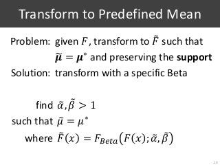
![[Voorhees, 2009]
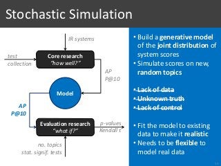
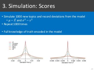
• Limited data
• Unknown truth (is H0 true?)
• No control over H0
• Cannot measure Type I error
rates directly
• Conflict rates at α=5%:
• AP: 2.8%
• P@10: 10.9%
1. Type I Errors?
28
𝑫 𝟐 + p-value𝑫 𝟏 + p-value
conflict?
S1
S2](https://image.slidesharecdn.com/065-180716151727/85/Stochastic-Simulation-of-Test-Collections-Evaluation-Scores-36-320.jpg?cb=1531754338)
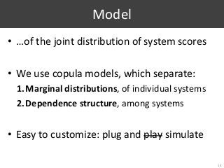
![[With simulation]
Same margins
1. Type I Errors
29](https://image.slidesharecdn.com/065-180716151727/85/Stochastic-Simulation-of-Test-Collections-Evaluation-Scores-37-320.jpg?cb=1531754338)
![[With simulation]
Same margins
1. Type I Errors
29](https://image.slidesharecdn.com/065-180716151727/85/Stochastic-Simulation-of-Test-Collections-Evaluation-Scores-38-320.jpg?cb=1531754338)
![[With simulation]
Same margins
1. Type I Errors
29](https://image.slidesharecdn.com/065-180716151727/85/Stochastic-Simulation-of-Test-Collections-Evaluation-Scores-39-320.jpg?cb=1531754338)
![[With simulation]
Same margins
1. Type I Errors
29](https://image.slidesharecdn.com/065-180716151727/85/Stochastic-Simulation-of-Test-Collections-Evaluation-Scores-40-320.jpg?cb=1531754338)
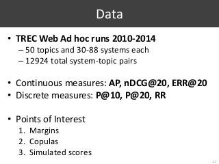
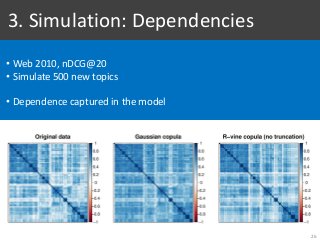
![[With simulation]
Same margins
• Type I errors at α=5% and 1%:
• AP: 4.9% and 0.9%
• P@10: 4.9% and 1%
1. Type I Errors
29
p-value
Type I
error?](https://image.slidesharecdn.com/065-180716151727/85/Stochastic-Simulation-of-Test-Collections-Evaluation-Scores-41-320.jpg?cb=1531754338)
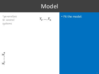
![[With simulation]
Same margins
• Type I errors at α=5% and 1%:
• AP: 4.9% and 0.9%
• P@10: 4.9% and 1%
Transformed margins
1. Type I Errors
30](https://image.slidesharecdn.com/065-180716151727/85/Stochastic-Simulation-of-Test-Collections-Evaluation-Scores-42-320.jpg?cb=1531754338)
![[With simulation]
Same margins
• Type I errors at α=5% and 1%:
• AP: 4.9% and 0.9%
• P@10: 4.9% and 1%
Transformed margins
1. Type I Errors
30](https://image.slidesharecdn.com/065-180716151727/85/Stochastic-Simulation-of-Test-Collections-Evaluation-Scores-43-320.jpg?cb=1531754338)
![[With simulation]
Same margins
• Type I errors at α=5% and 1%:
• AP: 4.9% and 0.9%
• P@10: 4.9% and 1%
Transformed margins
1. Type I Errors
30](https://image.slidesharecdn.com/065-180716151727/85/Stochastic-Simulation-of-Test-Collections-Evaluation-Scores-44-320.jpg?cb=1531754338)
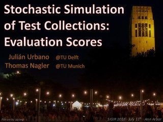
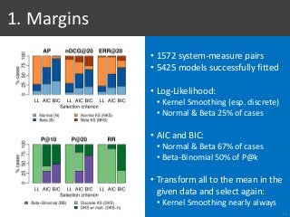
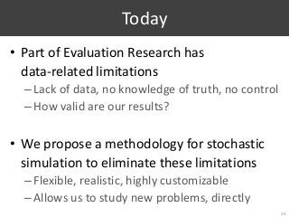
![[With simulation]
Same margins
• Type I errors at α=5% and 1%:
• AP: 4.9% and 0.9%
• P@10: 4.9% and 1%
Transformed margins
• Type I errors at α=5% and 1%:
• AP: 4.9% and 0.9%
• P@10: 5% and 1%
1. Type I Errors
30
p-value
Type I
error?](https://image.slidesharecdn.com/065-180716151727/85/Stochastic-Simulation-of-Test-Collections-Evaluation-Scores-45-320.jpg?cb=1531754338)
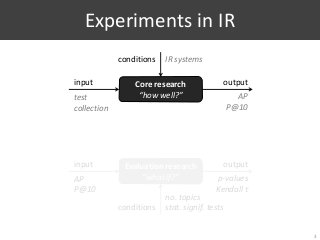
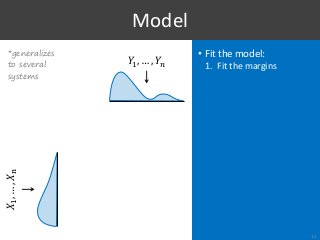
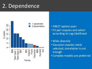
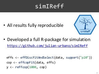
![2. Sneak Peak: Statistical Power and σ
31
[Webber et al, 2008]
• Show empirical evidence of the problem of sequential testing
• Limited data
• Unknown truth (true σ)](https://image.slidesharecdn.com/065-180716151727/85/Stochastic-Simulation-of-Test-Collections-Evaluation-Scores-46-320.jpg?cb=1531754338)


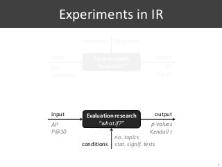
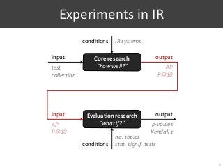
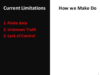
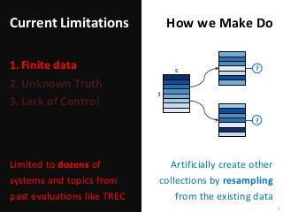
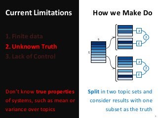
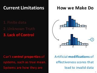
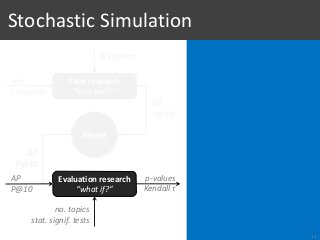
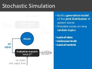
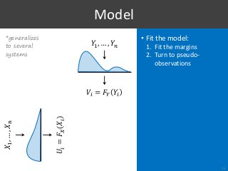
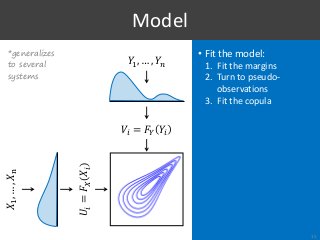
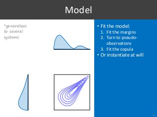
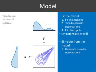
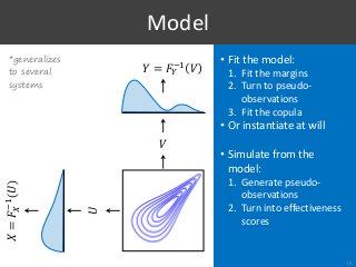
Part of Information Retrieval evaluation research is limited by the fact that we do not know the distributions of system effectiveness over the populations of topics and, by extension, their true mean scores. The workaround usually consists in resampling topics from an existing collection and approximating the statistics of interest with the observations made between random subsamples, as if one represented the population and the other a random sample. However, this methodology is clearly limited by the availability of data, the impossibility to control the properties of these data, and the fact that we do not really measure what we intend to. To overcome these limitations, we propose a method based on vine copulas for stochastic simulation of evaluation results where the true system distributions are known upfront. In the basic use case, it takes the scores from an existing collection to build a semi-parametric model representing the set of systems and the population of topics, which can then be used to make realistic simulations of the scores by the same systems but on random new topics. Our ability to simulate this kind of data not only removes the current limitations, but also offers new opportunities for research. As an example, we show the benefits of this approach in two sample applications replicating typical experiments found in the literature. We provide a full R package to simulate new data following the proposed method, which can also be used to fully reproduce the results in this paper.