Financial Formulae

Selected Financial Formulae

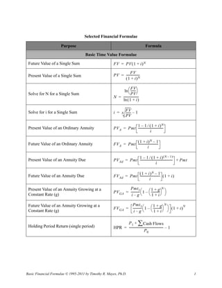
Purpose Formula

Basic Time Value Formulae

Future Value of a Single Sum FV = PV  1 + i  N

FV -
Present Value of a Single Sum PV = ------------------
 1 + iN

FV
ln  ------ -
Solve for N for a Single Sum  PV
N = --------------------
-
ln  1 + i 

Solve for i for a Single Sum FV – 1
i = N ------
-
PV

1 – 1   1 + i N
Present Value of an Ordinary Annuity PV A = Pmt ----------------------------------
-
i

 1 + i N – 1
Future Value of an Ordinary Annuity FV A = Pmt ---------------------------
-
i

1 – 1   1 + i   N – 1- 
Present Value of an Annuity Due PV Ad = Pmt -------------------------------------------- + Pmt
i

 1 + i N – 1
Future Value of an Annuity Due FV Ad = Pmt ---------------------------  1 + i 
-
i

Present Value of an Annuity Growing at a Pmt 1 1+g N
PV GA = ------------  1 –  -----------  
-
Constant Rate (g) i–g  1 + i 

Future Value of an Annuity Growing at a Pmt 1 1+g N
FV GA = ------------  1 –  -----------    1 + i 
N
-
Constant Rate (g) i–g   1 + i 

P 1 +  Cash Flows
Holding Period Return (single period) HPR = ---------------------------------------------- – 1
-
P0

Basic Financial Formulae © 1995-2011 by Timothy R. Mayes, Ph.D. 1


Purpose Formula

N
Holding Period Return with Reinvestment HPR Reinvest =   1 + HPRt  – 1
(for multiple sub-period returns) t=1

Basic Security Valuation Formulae

Dividend Discount Model (AKA, the Gordon D0  1 + g  D1
V CS = ----------------------- = ----------------
- -
Model) k CS – g k CS – g

Two-stage Dividend Discount Model
D0  1 + g1  1 + g1 n
Notes: This equation is too long for one line. V CS = -------------------------- 1 –  ----------------- +
g1 = Growth rate during high growth phase. k CS – g 1  1 + k CS
g2 = Growth in constant growth phase after n. D0  1 + g1   1 + g2 
n
n = Length of high growth phase. ------------------------------------------------
-
k CS – g 2
Assume g1 <> kCS and g2 < kCS ------------------------------------------------
-
n
 1 + k CS 

Three-stage Dividend Discount Model
Notes: 
n1 = Length of high growth phase. D0 n1 + n2
V CS = -------------------  1 + g 2  + ----------------  g 1 – g 2 
-
n2 = Periods until constant growth phase. k CS – g 2 2
n2 = n1 + length of transistion phase.

ROE
RE 1  ----------- – 1 -
Earnings Model EPS 1  k CS 
V CS = ------------ + ------------------------------------
- -
k CS k CS – g

Constant Growth FCF Valuation Model FCF 1
VOps = Value of Total Operations V Ops = ----------------
-
k CS – g
VDebt, VPref = Value of debt and preferred stock
VNon-Ops Assets = Value of non-operating assets V CS = V Ops – V Debt – V Pref + V Non – OpAssets

Sustainable growth rate
Note: b = retention ratio = 1 - payout ratio g = br
r = return on equity
D
Value of a Share of Preferred Stock V P = ----
-
kP



Purpose Formula

1 – 1   1 + kd N FV -
Value of a Bond on a Payment Date V B = Pmt ------------------------------------- + ---------------------
-
kd  1 + kd N

Quoted Price of a Bond on a Non-Payment
Date 
VB,0 = Value of bond at last payment date
V B  = V B 0  1 + k d  –   Pmt 
 = The fraction of the current period that has elaspsed

Basic Statistical Formulae

N
1
Arithmetic Mean (Average) X = ---
N
-  Xt
t=1

N
Geometric Mean (used for averaging returns,
growth rates, etc.)
G = N   1 + Rt  – 1
t=1

N
Expected Value (Weighted Average) EX =  t Xt
t=1

N
2
 t  Xt – X 
2
Variance X =
t=1

Standard Deviation 2
X = X

X
Coefficient of Variation CV = -----------
-
EX

N
Covariance  X Y =   t  Xt – X   Yt – Y  
t=1

 X Y
Correlation Coefficient r X Y = ------------
-
X Y

Beta (Note: M is the market portfolio, and i is  i M r i M  i  M
 i = ---------- = ----------------------
2
-
2
-
the security or portfolio) M M



Purpose Formula

Portfolio Formulae

N
Expected Return of a Portfolio E  RP  =  wi Ri
i=1

Using the covariance:
2 2 2 2 2
 P = w 1  1 + w 2  2 + 2w 1 w 2  1 2
Variance of a 2-security Portfolio
or, using the correlation coefficient:
2 2 2 2 2
 P = w 1  1 + w 2  2 + 2w 1 w 2 r 1 2  1  2

N N
Variance of an N-security portfolio Using the 2
Covariance
P =   w i w j  i j
i=1 j=1

Standard Deviation of a Portfolio 2
P = P

N
Portfolio Beta P =  wi i
i=1

95% Value at Risk (Variance/Covariance
Model)  VaR = 1.645  V p   p
Note: Vp is portfolio value

Capital Market Theory Models

 E  RM  – Rf 
Capital Market Line (CML) E  R P  = R f +  P -------------------------------
-
M

Capital Asset Pricing Model (CAPM)
Note: This is also the equation for the Security E  Ri  = Rf + i  E  RM  – Rf 
Market Line (SML)

Treynor’s Risk-adjusted Performance Ri – Rf
T i = ---------------
-
Measure i

Ri – Rf
Sharpe’s Risk-adjusted Performance Measure S i = ---------------
-
i



Purpose Formula

Jensen’s Alpha i =  Ri – Rf  – i  RM – Rf 

RP – RB
The Information Ratio IR P = ------------------
-
 RP – RB

M2 (Modigliani & Modigliani) Performance m
M =  ------  R i – R f  + R f
2
-
Measure  i 

Risk Premium = R i – R f
Fama’s Risk Decomposition
Risk =  i  R M – R f 
Notes:
Ri = Portfolio Return Selectivity = Risk Premium – Risk
RM = Market Return Managers Risk =   i –  T   R M – R f 
Rf = Risk-free Rate Investors Risk =  T  R M – R f 
i = Portfolio Beta
i
T = Target Beta Diversification =  ------ –  i  R M – R f 
-
 M 
Net Selectivity = Selectivity – Diversification
Brinson, Hood, and Beebower Additive N
Attribution Model
Notes:
At =   w i t – w i t   R i t – R t 
i=1
At = Overall Allocation Effect
N
St = Overall Selection Effect
It = Overall Interaction Effect
St =  wi t  Ri t – Ri t 
i=1
wi,t = Weight of Sector i in portfolio t
bars over variables represent benchmark N
weights and returns. It =   wi t – wi t   Ri t – Ri t 
i=1

Options and Futures Valuation Models
– rt
C = SN  d 1  – Xe N  d 2 
where:
Black-Scholes European Call Option S
ln  --  +  r + 0.5 t
2
-
Valuation Model  X
d 1 = ---------------------------------------------------
-
 t
d2 = d1 –  t



Purpose Formula

Black-Scholes European Put Option Valuation
Model (see above for d1 and d2) P = Xe – rt N  – d 2  – SN  – d 1 

C = P + S – Xe – rt
Put-Call Parity for European Options with No
or,
Cash Flows
P = C + Xe – rt – S

pC u +  1 – p C d
C = ---------------------------------------
Single-period Binomial Option Pricing Model 1 + r
for Call Options (r is the risk-free rate, u is the where,
up factor, and d is the down factor) r–d
p = -----------
-
u–d

pP u +  1 – p P d
P = --------------------------------------
-
1 + r
Single-period Binomial Option Pricing Model
for Put Options where,
r–d
p = -----------
-
u–d
Cost of Carry Model for Pricing Futures
Contracts (CC is the carrying costs as a % of T F0 = S 0 e CC  t 
the spot price)
Bond Analysis Formulae

N
Macaulay’s Duration on a Payment Date (for Ct  t 
immunization). Note: Ct is the cash flow in   1 + i -t
----------------
t=1
period t, i is the yield to maturity D = --------------------------
-
Bond Price

Modified Duration (for price volatility) on a D
D Mod = ---------------
Payment Date 1 + i

N Cf t
1
-----------------   t 2 + t  ----------------
- -
Convexity on a Payment Date  1 + i 2 t = 1  1 + i t
C = --------------------------------------------------------------------
-
Bond Price

i
The n-period forward rate given two spot rates  1 + Ri 
(note that i > j, and n = i - j) t + jRn = n -------------------- – 1
j
 1 + Rj 



Purpose Formula

Bank Discount Yield for discount securities
FV – PP 360
(FV = face value, PP = purchase price, m = BDY = --------------------  --------
- -
FV m
periods per year)
FV – PP 365 FV 365
Bond Equivalent Yield for discount securities BEY = --------------------  -------- = BDY  ------  --------
- - - -
PP m PP 360
(see definitions for BDY)

Capital Budgeting Decision Formulae

N
Cf t
Net Present Value (NPV) NPV =  -----------------t – IO
1 + i
t=1

N
Cf t
Profitability Index (PI)  -----------------t
1 + i
t=1 NPV + IO NPV
PI = -------------------------- = ------------------------ = ----------- + 1
- - -
IO IO IO
Internal Rate of Return (IRR). Note: This is a
N
trial and error procedure to find the i that Cf t
makes the equality hold (i.e., what discount
0 =  -----------------t – IO
1 + i
t=1
rate makes the NPV = 0).

N
N – t
Modified Internal Rate of Return (MIRR).  Cft  1 + i 
t=1
N
MIRR = --------------------------------------------- – 1
-
IO
Stock Market Index Construction Formulae
Price-weighted Average (e.g., DJIA) N
Note: The divisor (Div) at period 0 is equal to
the number of stocks in the average. It will be 1 Pj
j=
adjusted for stock splits or any other corporate PWA t = -------------
-
Div t
action that results in a non-economic change
in the stock price.



Purpose Formula

Capitalization-weighted Index (e.g., S&P
500) N
Note: The divisor (Div) at period 0 is the  Pj Qj
divisor that makes the initial level of the index j=1
CWI t = --------------------
equal to the desired starting point. It will be Div t
adjusted for any corporate action that results
in a change in market capitalization.
Equally-weighted Arithmetic Index (e.g.,
VLA) N
Note: At period 0 the index is set to some P j t
starting value (e.g., 100). To calculate the
EWAI t = EWAI t – 1    ---------------  N
 P j t – 1
j=1
index for any day, multiply the average %
change by the previous index level.

Equally-weighted Geometric Index (e.g., N
P j t
VLG)
Note: See note above
EWGI t = EWGI t – 1  N  ---------------
P j t – 1
j=1

Corporate Financial Formulae
Net Operating Profit After Taxes (NOPAT) NOPAT = EBIT  1 – t 

Net Operating Working Capital (NOWC) NOWC = Op. C.A. – Op. C.L.

Operating Capital (Op. Cap.) Op. Cap. = NOWC + NFA

Free Cash Flow (FCF) FCF = NOPAT – Net Investment in Op. Cap.

Economic Value Added (EVA) EVA = NOPAT –  Op. Cap.  Cost of Cap. 

Beta of a Leveraged Firm L = U  1 +  1 – t   D  S  

MM Value of Firm, No Corporate Taxes VL = VU = SL + D

MM Value of Firm With Corporate Taxes V L = V U + tD

 1 – tC   1 – tS 
Miller Value of Firm with Personal Taxes V L = V U + 1 – ------------------------------------ D
-
 1 – tD 

Miscelaneous Formulae



Purpose Formula

Margin Call Trigger Price
Note: IM% is the initial margin supplied,
IM% – 1-
MM% is the maintenance margin P M = -----------------------  P 0
requirement, P0 is the initial value of the MM% – 1
portfolio
Percentage gain to recover (% GTR) from a 1 -
%GTR = ---------------- – 1
loss (%L) 1 – %L


Financial Formulae

Recommended

Recommended

More Related Content

Viewers also liked

Viewers also liked (8)

Financial Formulae