This document provides a summary of analysis from the author's Macro Strategy Review publications from 2014 to 2015. It discusses the author's approach of combining fundamental and technical analysis. As an example, in 2014 the author correctly predicted a rally in the US dollar based on signals from the euro currency and implications for emerging markets. The summary highlights several insights the author provided regarding the dollar, euro, commodities, and emerging markets. It positions the Macro Strategy Review as a valuable resource that helps navigate challenging markets by incorporating both fundamental and technical analysis.

![Macro Strategy Review www.forwardinvesting.com18
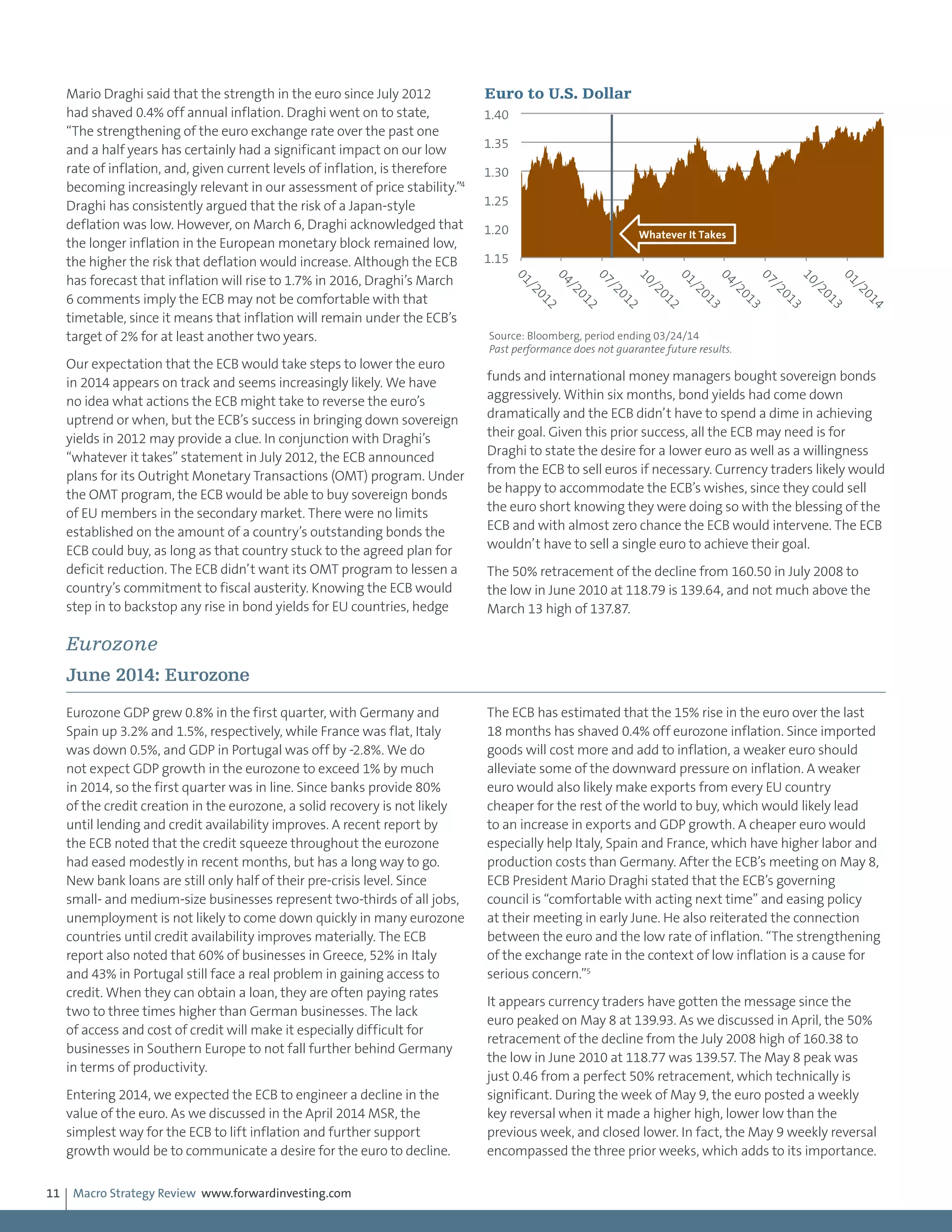
dollar strength. According to the International Monetary Fund,
$650 billion has flowed into emerging markets as a result of
quantitative easing by the Federal Reserve. There is a significant
risk that some of this money will flow out of emerging economies
as their currencies depreciate. A rush for the exit has the potential
of igniting a currency crisis as affected central banks are forced to
defend their currency through direct intervention or interest
rate increases.
According to the Bank for International Settlements, more than
two-thirds of the $11 trillion in cross-border bank loans are
denominated in dollars and an unknown amount is not hedged.
This has the potential to be a big problem since nonhedged dollar
debt becomes more expensive as the dollar rises. For instance, if the
dollar rises by 12%, which it has since May, a $100 million loan that
is nonhedged may now be effectively $112 million if the currency
of the loan holder has fallen 12%. This is another aspect of why
the depreciation of the yen and euro amounts to those countries
exporting the very deflation they are attempting to ward off in
their own economies. The volatility in the currency market that the
BOJ and ECB have initiated is likely to intensify in coming months.
If it does, it is easy to see how it could spill over into global equity
markets, which have greeted every central bank intervention by
lifting stock valuations.
Emerging Markets
February 2015: U.S. Dollar and Foreign Currency
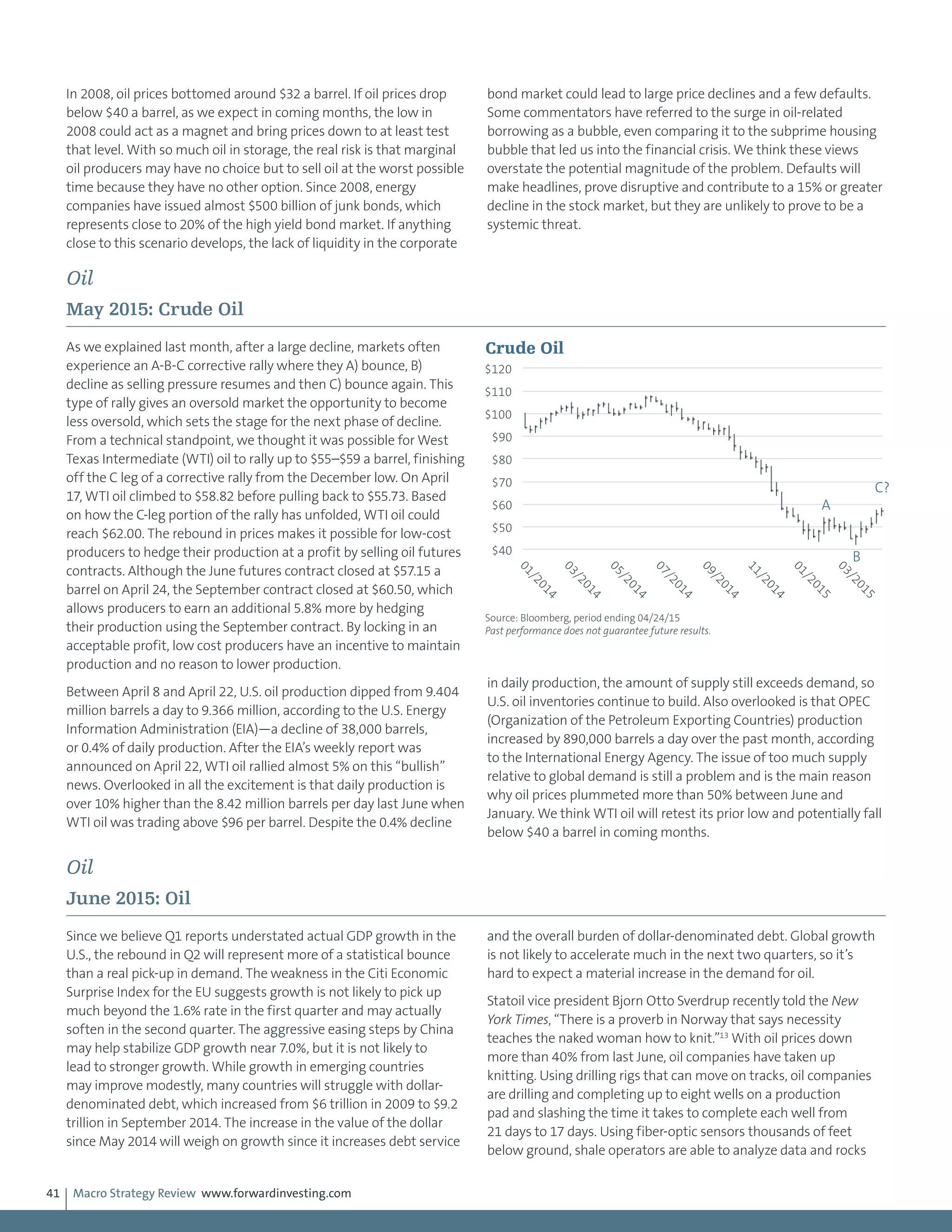
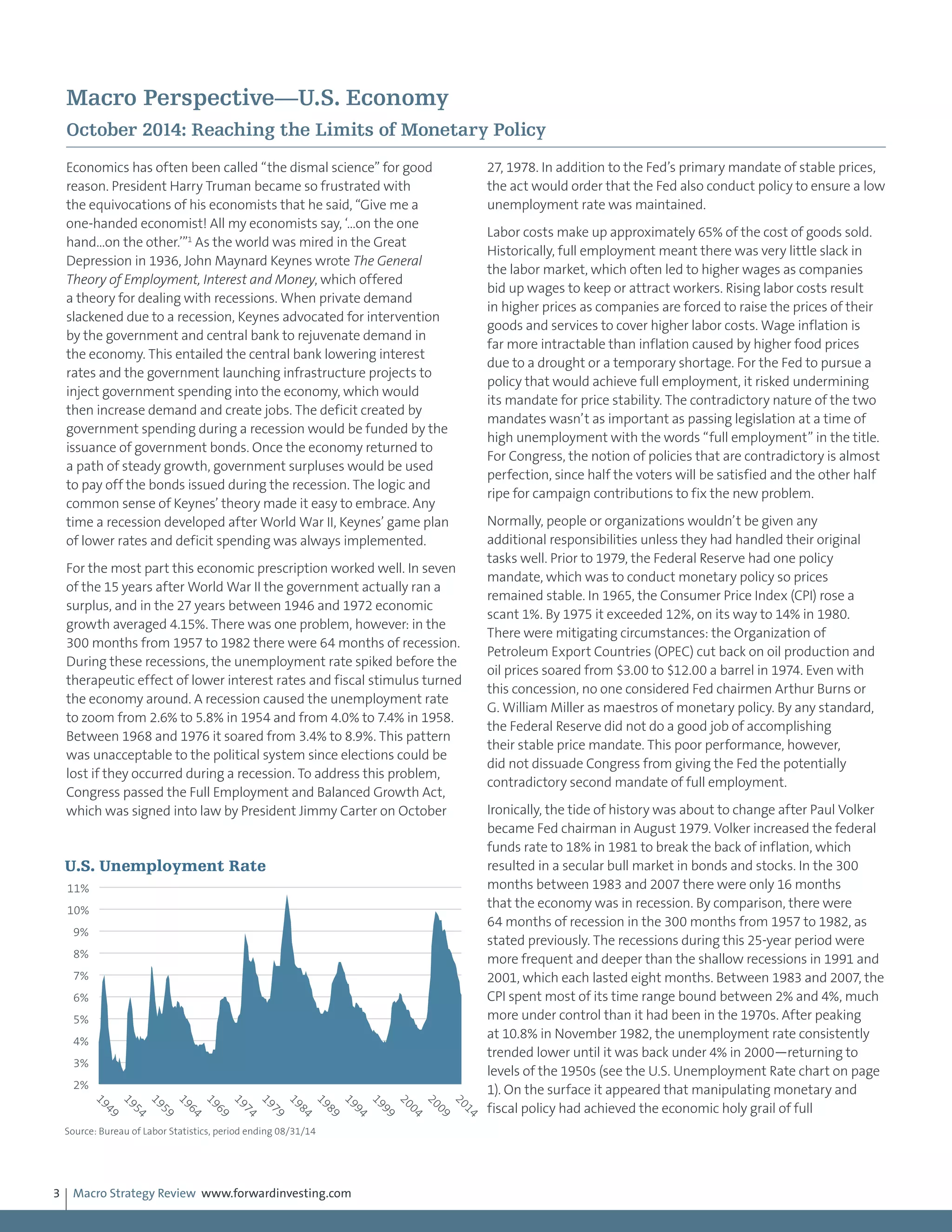
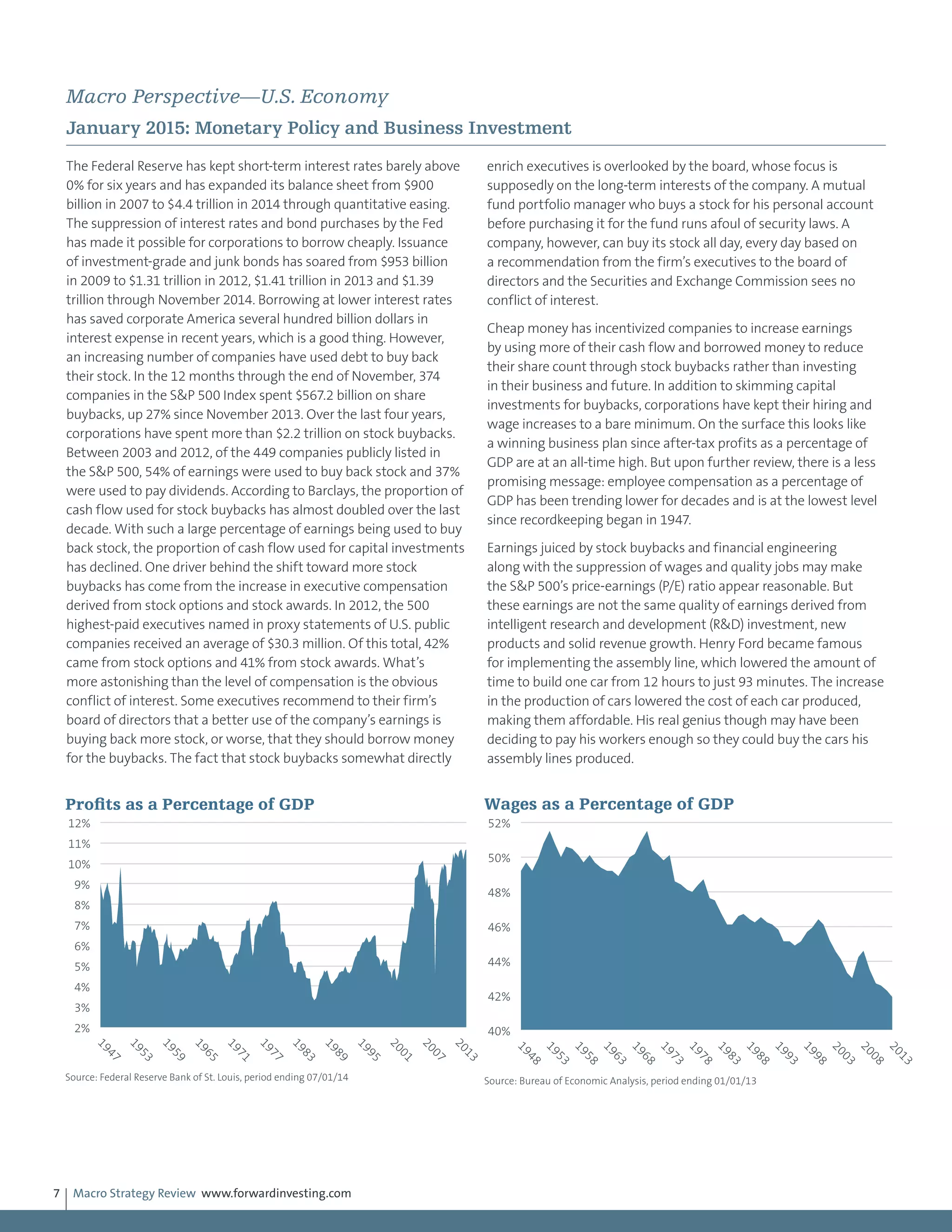
In the April 2014 MSR we wrote, “The collateral damage that might
flow from a weaker euro and stronger dollar could include renewed
weakness in emerging market [EM] currencies with current account
deficits and another decline in gold and a range of commodities,
since a stronger dollar is likely to increase deflationary pressures in
the global economy. There is a lot of debt denominated in dollars
and most commodities are priced in dollars.” The euro experienced
a three week key reversal the week of May 9, 2014, which we
discussed in the June 2014 MSR. The technical key reversal in the
euro coincided with the beginning of the rally in the dollar. Based on
the J.P. Morgan basket of emerging market currencies (EMCI), dollar
strength has translated into a decline of 13.3% as this is written on
January 26. Since May 2014, the S&P Goldman Sachs Commodity
Index (GSCI) has declined by 41.5%. Certainly, a large portion of the
loss was due to the drop in oil, but many other commodities have
fallen, just less dramatically. Copper has declined -17.3% after falling
from $3.05 a pound last May to $2.52. As noted in previous MSRs,
we expected gold to break below its support at $1,180 as the dollar
strengthened. Gold bottomed on November 7, 2014, at $1,132
-10%
-8%
-6%
-4%
-2%
0%
2%
4%
6%
8%
11/02/1201/02/1303/02/1305/02/1307/02/1309/02/1311/02/1301/02/1403/02/1405/02/1407/02/1409/02/1411/02/14
South Korea Taiwan Singapore China
U.S. Dollar vs. South Korea Won, Taiwan Dollar,
Singapore Dollar and China Yuan
Source: Bloomberg, period ending 11/21/14
Past
performance
does
not
guarantee
future
results.
75
80
85
90
95
100
105
110
01/2011
07/2011
01/2012
07/2012
01/2013
07/2013
01/2014
07/2014
01/2015
J.P. Morgan EM Currency Index
Source: J.P. Morgan, period ending 01/22/15
Past performance does not guarantee future results.
Taper Talk
Dollar Rally
350
400
450
500
550
600
650
700
750
01/2012
07/2012
01/2013
07/2013
01/2014
07/2014
01/2015
S&P GSCI
Source: Standard & Poor's, period ending 01/23/15
Past performance does not guarantee future results.
Dollar Rally](https://image.slidesharecdn.com/3ca54fc7-5ea5-4e4e-85bb-b7d4f20a37b2-150930200801-lva1-app6891/75/Macro-Strategy-Review-Summary-Jan-2014-Aug-2015-18-2048.jpg)
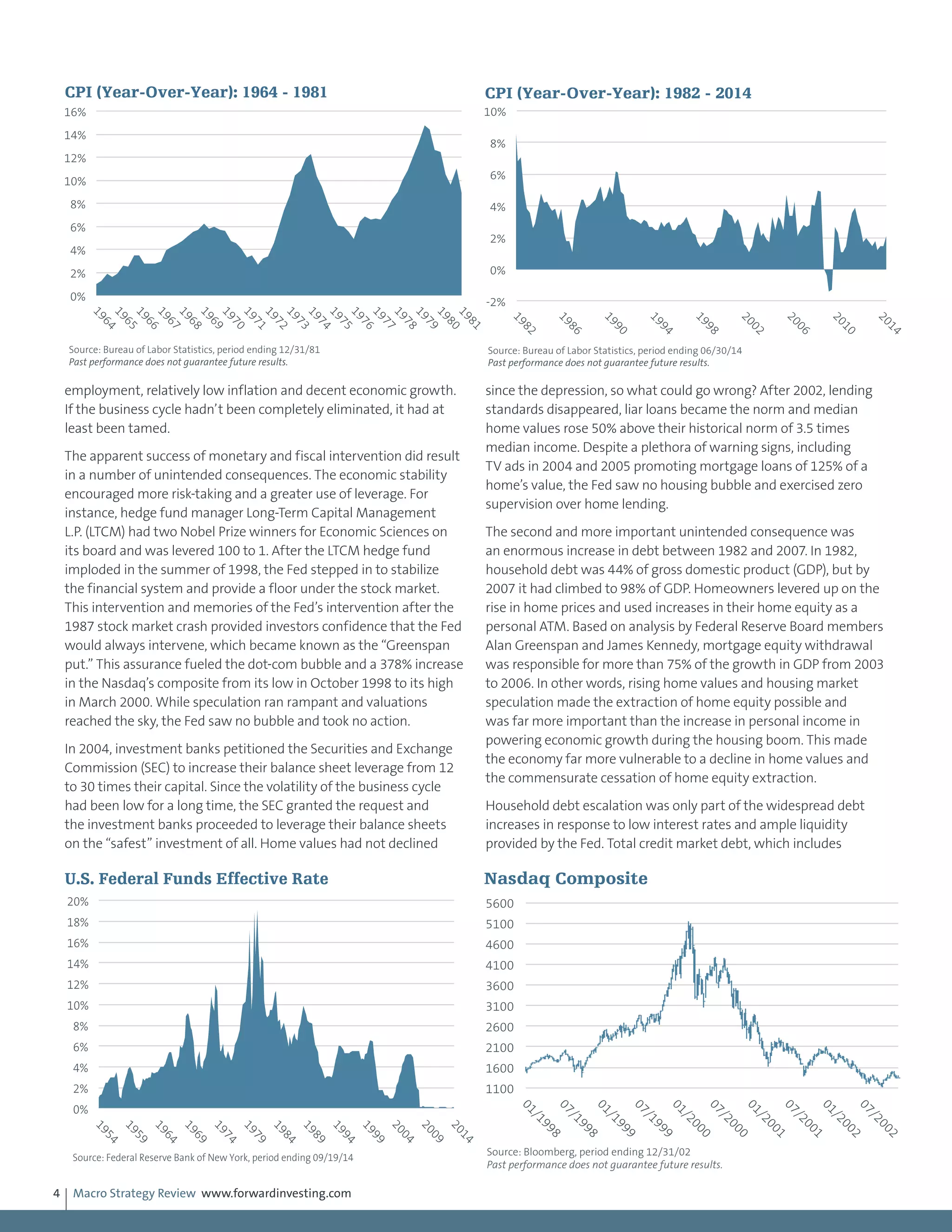
![Macro Strategy Review www.forwardinvesting.com20
Information Administration. Since these commodities are priced in
dollars, we expected the decline in the yen to increase the cost of
these imports, resulting in more inflation and a larger trade deficit.
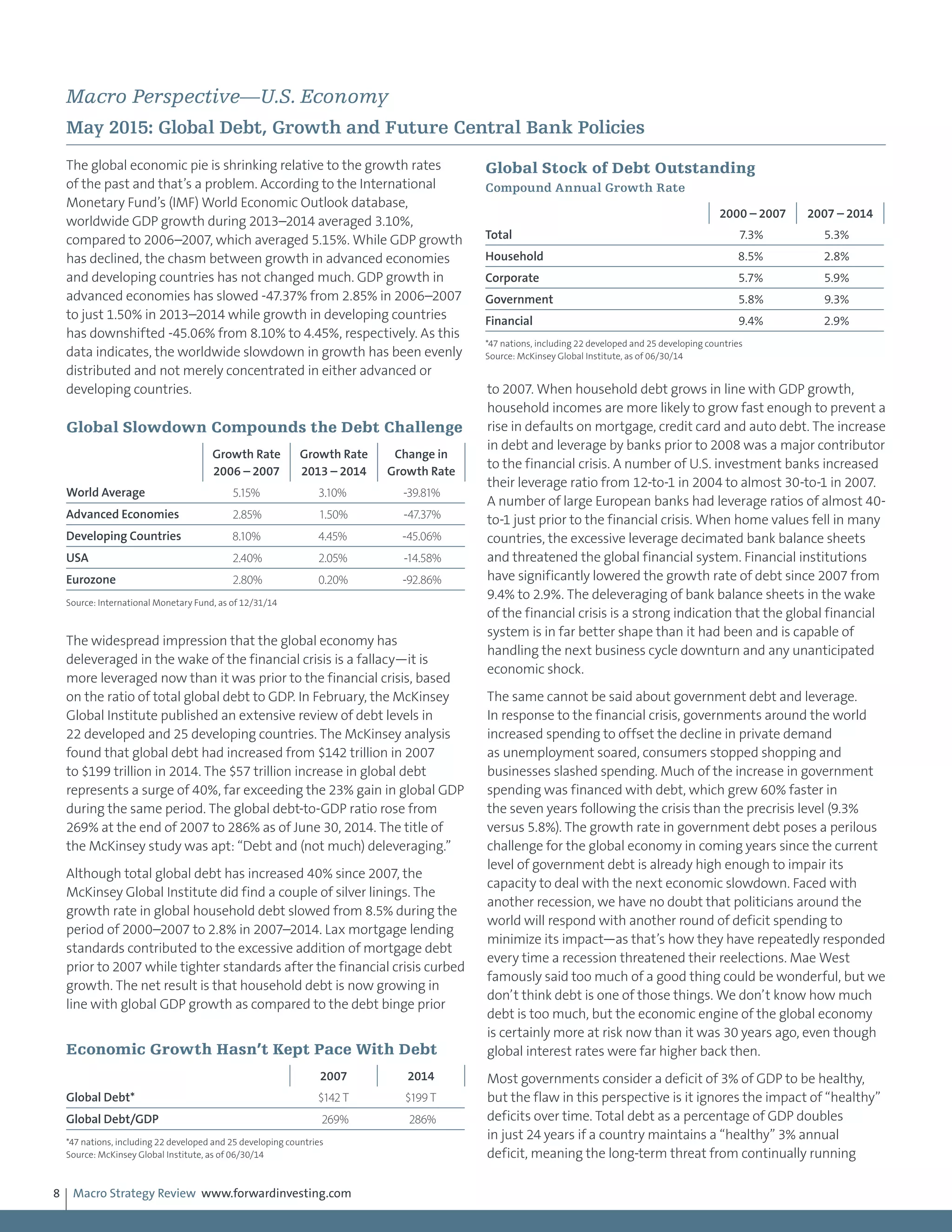
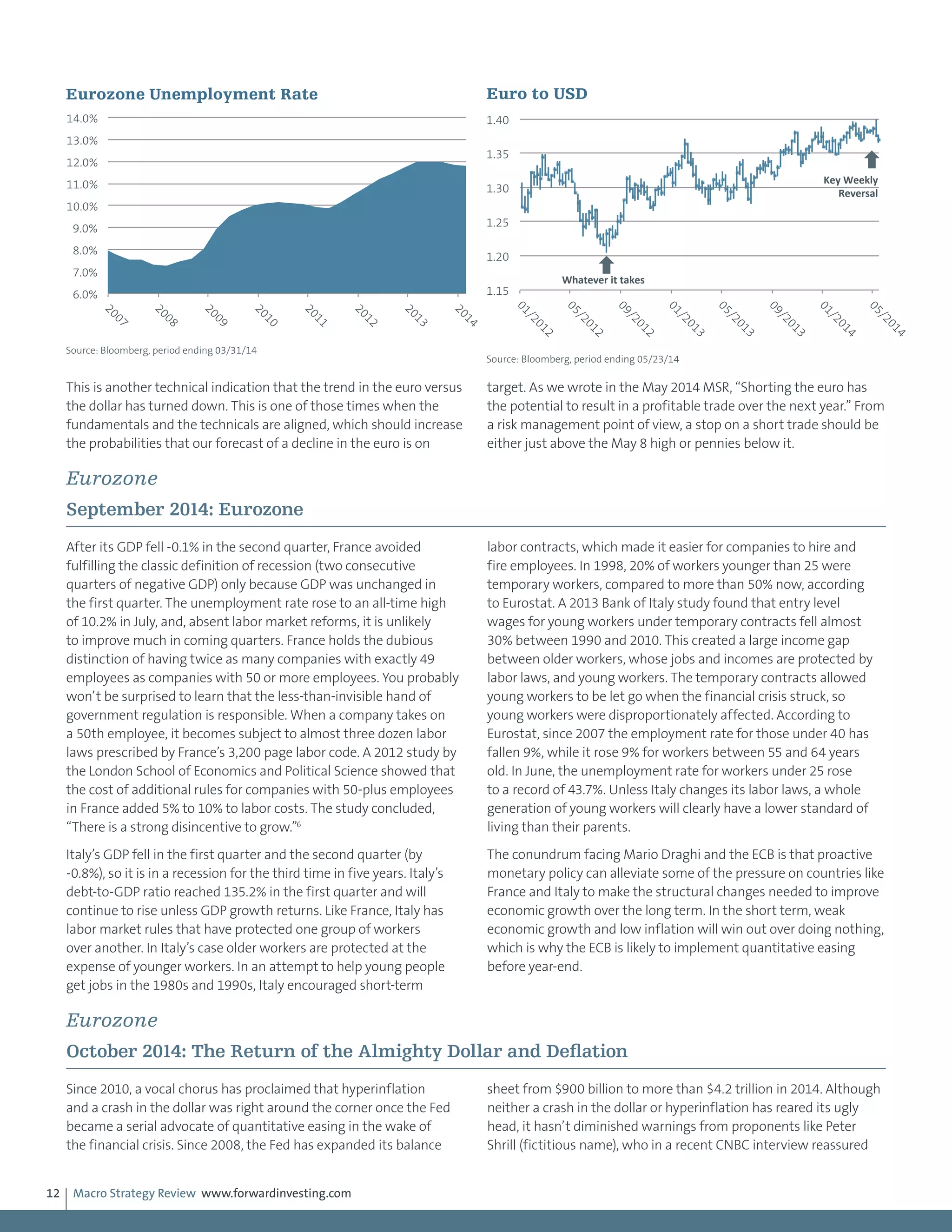
In May, Japan’s Consumer Price Index (CPI) was 3.7% higher than in
May 2013. As of March 31, 2014 (latest data available), Japan’s trade
deficit as a percentage of GDP was the largest in decades. Prime
Minister Shinzo- Abe has succeeded in reversing deflation, but he
may have succeeded too well since the cost of living is rising faster
than the increase in wages. This may hurt future consumption,
resulting in slower GDP growth in coming quarters. If Japan’s
economy does not shows signs of recovering from the tax increase
before year-end, the Bank of Japan may instigate another round of
QE to cheapen the yen further and boost Japan’s stock market.
Japan
December 2014: Japan
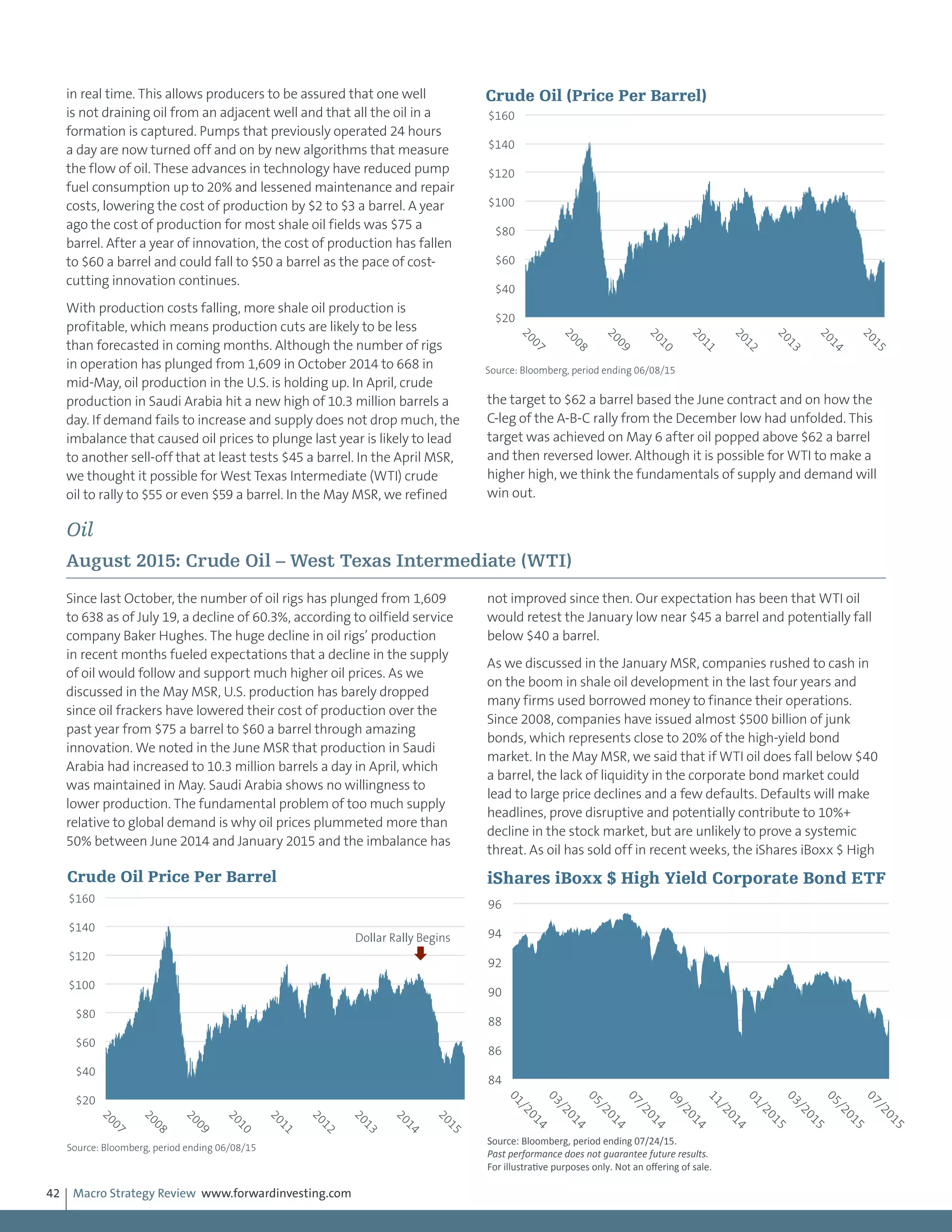
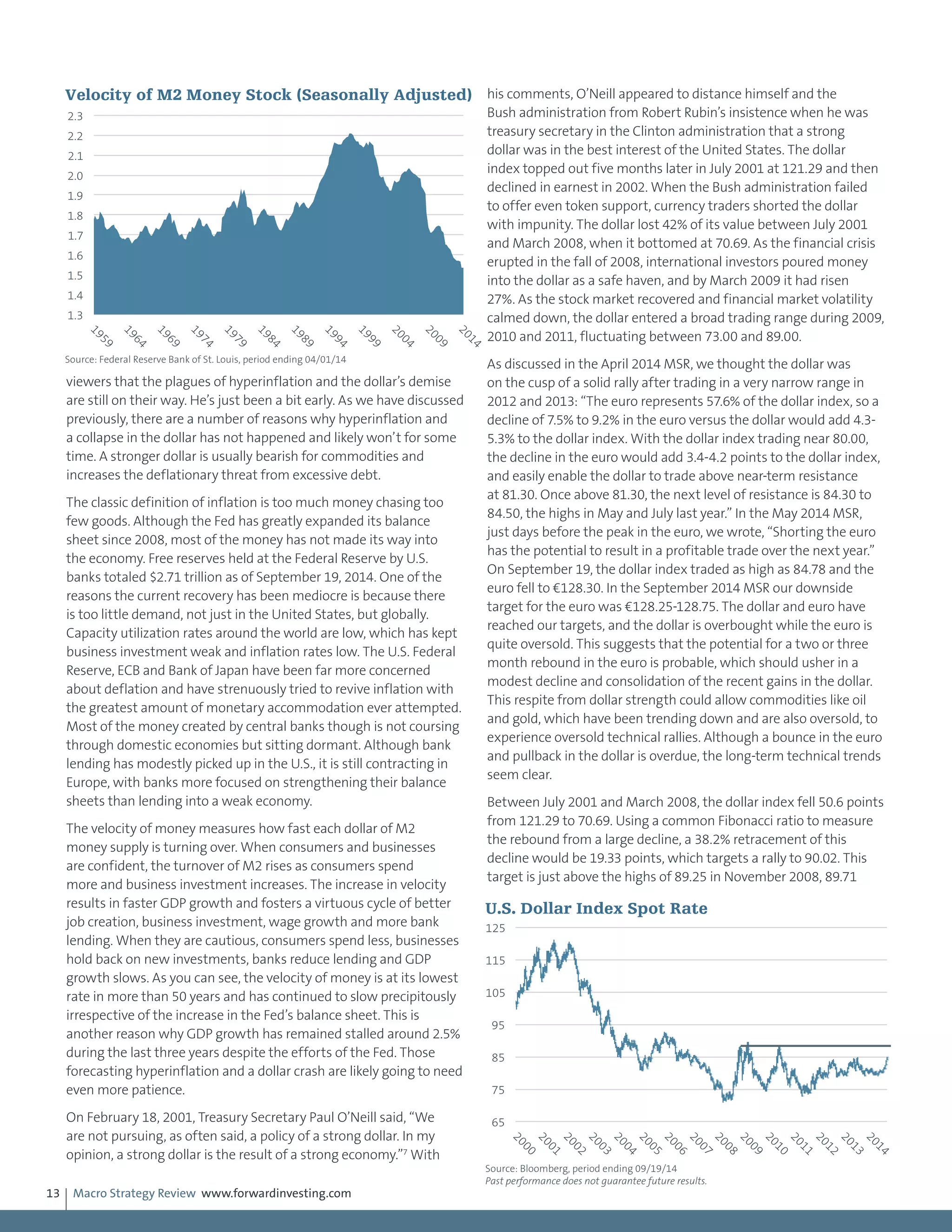
Japan’s newest round of quantitative easing, tax cuts and currency
devaluation was triggered by a -1.6% decline in third quarter GDP
after its economy contracted -7.3% in the second quarter. The
weakness in the second quarter was prompted by an increase
in Japan’s sales tax from 5% to 8% on April 1. As we noted in the
November 2013 MSR, “As consumers rush to buy before April
in order to save 3% on their purchases…first quarter [2014] GDP
will be lifted by the surge in consumer demand, only to weaken
significantly in the second quarter. This will be the first real test of
the durability of Abenomics.” While the first quarter strength of
6.7% and second quarter weakness was predictable, the contraction
in the third quarter illustrates how fragile the Japanese economy
remains. In the August 2014 MSR we wrote, “If Japan’s economy
does not show signs of recovering from the tax increase before
year-end, the Bank of Japan may instigate another round of QE to
cheapen the yen further and boost Japan’s stock market.”
With the contraction in the second and third quarters, Japan has
entered its fourth recession since 2007. The BOJ vote to increase
its QE program was a close 5 to 4, however, since some members
are concerned about the precariousness of Japan’s long-term fiscal
health. As Japan’s total debt-to-GDP ratio is a mind-blowing 640%,
their concern is more than justified.
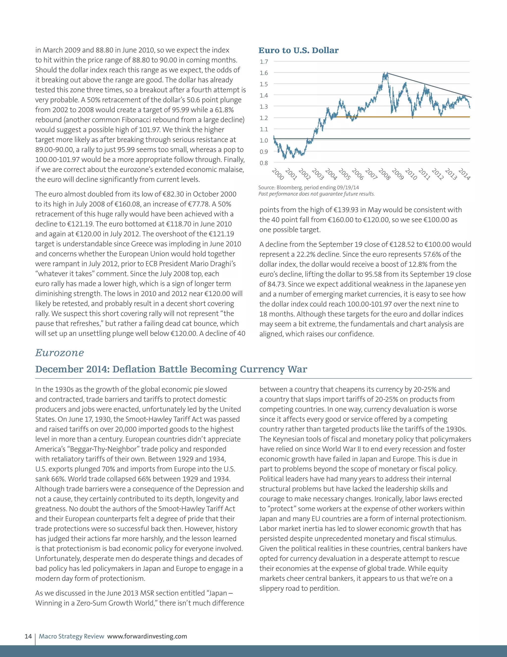
Real household income, which adjusts for inflation, has declined for
15 consecutive months and has dropped from an increase of almost
3% in the first half of 2013 to -6.0% as of September 30, 2014.
Although wages rose for the seventh straight month in September
and were up 0.5% from September 2013, the improvement in
wages still lagged the 3.2% increase in Japan’s consumer price index
(CPI) in September. The purchasing power of the average Japanese
worker continues to worsen. In fact, a BOJ survey released in
October found that only 4.4% of households said they were better
off than a year ago. As consumers account for about 65% of Japan’s
GDP, their finances and outlook are important.
-3
-2
-1
0
1
2
3
4
1999
2000
2001
2002
2003
2004
2005
2006
2007
2008
2009
2010
2011
2012
2013
Japan CPI (Year-Over-Year Change)
Rising Faster Than Incomes
Source: Ministry of Internal Affairs, period ending 05/31/14
Past performance does not guarantee future results.
-10%
-8%
-6%
-4%
-2%
0%
2%
4%
6%
03/31/07
09/30/07
03/31/08
09/30/08
03/31/09
09/30/09
03/31/10
09/30/10
03/31/11
09/30/11
03/31/12
09/30/12
03/31/13
09/30/13
03/31/14
09/30/14
Japan GDP Growth (Year-Over-Year)
Source: Economic and Social Research Institute, period ending 09/30/14
500%
520%
540%
560%
580%
600%
620%
640%
660%
1999
2000
2001
2002
2003
2004
2005
2006
2007
2008
2009
2010
2011
2012
2013
2014
Japan Debt Oustanding as a Percentage of GDP
Source: Morgan Stanley Research, period ending 06/30/14
-8.0%
-6.0%
-4.0%
-2.0%
0.0%
2.0%
4.0%
6.0%
8.0%
10.0%
01/01/07
07/01/07
01/01/08
07/01/08
01/01/09
07/01/09
01/01/10
07/01/10
01/01/11
07/01/11
01/01/12
07/01/12
01/01/13
07/01/13
01/01/14
07/01/14
Japan Household Income (Year-Over-Year)
Source: Ministry of Internal Affairs, period ending 09/30/14](https://image.slidesharecdn.com/3ca54fc7-5ea5-4e4e-85bb-b7d4f20a37b2-150930200801-lva1-app6891/75/Macro-Strategy-Review-Summary-Jan-2014-Aug-2015-20-2048.jpg)